A new model of random graphs, the random dot product graph (RDPG) is described. .... same random graphs, it turns out that the dimension d of the vectors needed ... computed by first rotating the first vector to the x-axis, thus eliminating all ... In order to correct for the changing order of the graphs, we will scale the log.
Modeling Interstate Alliances with Constrained Random Dot Product Graphs David J. Marchette1 and Carey E. Priebe2 1
Naval Surface Warfare Center, Code Q21, Dahlgren, VA 22448 Applied and Mathematical Statistics, Johns Hopkins University, Baltimore, MD 21218
2
Summary A new model of random graphs, the random dot product graph (RDPG) is described. This model is well suited to social networks, since it defines the edges in the graph in terms of a vector of “attributes”. The edge probabilities are modeled as the dot product of vectors associated with the vertices. A small set of distinct vectors is used, allowing the automatic grouping of vertices according to their attributes. We discuss various issues of model fitting and model selection for the reduced vector set version of the RDPG. We extend the basic model to model time series of graphs, and illustrate the model through application to a time series of graphs defined by the alliances between nation states. Keywords: Random Graphs, Social Networks, Time Series of Graphs
1
1
Motivation
A graph is a pair G = (V, E), where V = {v1 , . . . , vn } is a set of vertices and E, the edge set, is a set of unordered pairs of distinct vertices (we do not allow loops in our graphs). The order of the graph is |V | and the size is |E|. As is the convention, we will write vw for {v, w} ∈ E. In this paper we will consider a time series of graphs, that is, a collection of graphs indexed by (discrete) time. There are two viewpoints that one could take on time series of graphs. Dynamic graphs are graphs that change in time. Usually this means that the edge set changes in time: at each time step an edge may be added or removed. We will not concern ourselves with dynamic graphs. Instead, we assume that there is a (possibly time dependent) random model from which the graphs are drawn, and at each time t a new graph is drawn from this model (possibly depending on graphs drawn prior to t). Throughout our discussion, the vertex set V will be fixed, and it is labeled, meaning that there is a known 1-1 correspondence between the vertices of the graph at time t and the one at time t + 1, allowing us to match up the vertices over time. In this paper we focus primarily on model selection in the Random Dot Product Graph model of Kraetzl et al. and ?. vector of attributes to each vertex, such that the probability of an edge is equal to (a function of) the dot product of the vectors. In this paper we consider the following model selection problem: can we choose a small number (K � |V |) of distinct vectors to fit to the graph, so that each vertex is associated with one of these vectors? In this manner we obtain a natural grouping of vertices according to the selection of the vectors. There are several reasons to consider this problem: 1. Regularization: we reduce (dramatically) the number of parameters of the model. This reduces variance. 2. Interpretation: the much smaller number of vectors can make the interpretation and understanding of the graph much easier. 3. Clustering: the model provides a natural clustering of the vertices, which can be exploited to better understand the natural groupings of the data underlying the graph. While the selection of dimension (d) for the vectors is also necessary, we provide a rule-of-thumb formula for the dimension as a function of K, and suggest that practitioners err on the side of smaller values for d, unless there is a compelling a priori or scientific reason to choose a larger dimension. This aids in the interpretation (and visualization) of the model, as well as providing further regularization.
2
0 or NA 1 2 3
Table 1: Alliance codes in the alliance dataset. No alliance Defense pact intervene militarily if partner attacked Neutrality remain militarily neutral if partner attacked Nonaggression pact consultation and/or cooperation in a crisis
We consider a time series of graphs defined in terms of alliances between countries. We investigate data representing alliances between a total of 173 nations collected from 1816 to 2000. The data are available at cow2.la. psu.edu (see Gibler and Sarkees [2004]), and we provide a processed dataset (with more attributes than are considered in this paper) at www.ams.jhu. edu/~marchette/igo.tgz. In this latter dataset, there are a total of 214 nations, since while some of these do not have alliances, they do have other attributes such as trade. For each pair of nations, alliance is coded as in Table 1. There are some missing values in the interstate alliance data, and in this study we treat these as missing edges. Various methods for imputing the missing values could be considered instead. While the edges are colored by alliance type (see Table 1), we will consider only the simplified graph with binary edges: existence or absence of an alliance. We will construct an alliance graph for each year. Thus the vertices of the graph will consist of the 173 nations, and there will be an edge between two vertices if the corresponding nations had an alliance during the year. This produces a time series of graphs. We will describe a new model of random graphs and apply this model to the time series.
2
Random Dot Product Graphs
We do not believe that most interesting random graphs have independent edges, and so we seek a model that relaxes this requirement. A simple model, which has some interesting (and possibly relevant) properties is the random dot product model. A random dot product graph (RDGP) is a random graph model containing Erd¨ os-Reny´ı random graphs Bollob´ as [2001] as a sub-model, in which each vertex v is assigned a vector xv ∈ Rd . The probability of an edge from v to w is a function of the dot product of the vectors: pvw = f (x0v xw ). In this paper we will set f to be a simple threshold: 0 x≤0 f (x) = x 0≤x≤1 1 x≥1
3
The vectors xv are fixed, and new graphs are drawn from the collection of all graphs on n vertices according to the edge probabilities defined above. It should be noted that in addition to being a generalization of the Erd¨ osReny´ı random graph, the RDPG is a generalization of random intersection graphs (Karonski et al. [1999]) and a sub-model of latent position models (Hoff et al. [2002], Hoff [2005]). The motivation for these come from social networks applications. It seems reasonable to assume that individuals have a collection of attributes which (to a large extent) define the probabilities of connection with others. For example, in a friendship graph the attributes might correspond to interest areas and personality, and the probability of an edge (friendship) between two individuals is largely driven by the overlap of their interests and the compatibility of their personalities. This is admittedly a simplification. It is not clear that in real problems such attribute vectors can be reliably identified. However, the model is a reasonable approximation, and one can proceed to fit the model without assuming any particular interpretation to the vectors. This will be our philosophy in this work. One reason for choosing the RDPG over the distance model described in Hoff et al. [2002] is parsimony for a certain class of graphs. We are interested in finding groupings within the vertices, and the RDPG allows us to define these groups as being those which share the same vector. While (with suitable assumptions on the probabilities) the two models can be used to define the same random graphs, it turns out that the dimension d of the vectors needed in the distance model can be much larger for certain cases than is necessary for the dot product model. As we will see, a dimension of d = 2 is adequate for the problem we consider. Although computationally challenging, fitting the vectors to a given graph or set of graphs is relatively straightforward. Scheinerman (Kraetzl et al., Scheinerman [2005] and Scheinerman and Tucker [2007]) gives a linear algebra method that tries to minimize the Frobenious norm for the edge probabilities, and maximal likelihood is straight forward due to the fact that the probabilities are conditionally independent, given the vectors. Thus, the likelihood is: Y a 1−a L= (x0i xj ) ij (1 − x0i xj ) ij . (1) i6=j
Here, ai,j is the ijth element of the adjacency matrix. For a graph G = (V, E), a partition is a collection of subsets of vertices P = {P1 , . . . , Pk } such that Pi ∩ Pj = ∅ for i 6= j and ∪Pi = V . We will assume the number of partitions K is known a priori. In a social network context, these groups might be club membership, interest groups, religious affiliation, or some unobserved grouping that one would like to discover. Thus, we are provided with a set of partition labels L, and seek a map
4 h : V → L. For a fixed (known) value of K, a maximum likelihood estimate can be obtained via the following algorithm: 1. Start with an initial set of vectors {xj }K j=1 and an initial assignment of vectors to vertices. 2. For each vertex vi (sequentially), select the vector xj for which, after reassignment of the vector to the vertex vi , the likelihood is maximized. 3. With the assignment fixed, select the vectors to maximize the likelihood. 4. Repeat from 2 until convergence. Note that the assignment in 2 is sub-optimal: we only procede through the vertices once sequentially, making the current assignment conditional on the previous assignments for the later vertices and the current assignments of the previous vertices in the list. This can be improved, presumably resulting in an algorithm that produces fewer iterations, at the expense of extra computation at this step. We will not consider these trade-offs here. We have several model selection problems in this work. First, one must decide on the dimensionality d of the attribute vectors xi . In a particular application, this should be in part driven by scientific considerations. One may hypothesize that there are two main factors defining the relationships, and thus choose d = 2 and observe the model fit. It should be noted that we want to pick d as small as possible, due to the additional variance in the estimators as the dimension increases. For the purpose of this work we will set d = 2. Investigation of higher values of d showed no significant improvement in the models. There is a rule-of-thumb that can be derived to select the value of d appropriate for a given K. The idea is to match up the number of values fit with the number of parameters available. Assume that each vector is assigned to at least two vertices. In this case, the entire dot product matrix must be fit, including the diagonal. Thus we have � � K +K (2) 2 values to be fit. One might consider that there are Kd parameters, however the dot products are invariant to rotations (the orthogonal group O(d)). We’ll consider an upper bound on the number of parameters to be (K − 1)d + 1
(3)
5
computed by first rotating the first vector to the x-axis, thus eliminating all but one (the length of the vector) of the parameters for this vector. We have implicitly assumed that d > 1 here. Equating (2) and (3) we have d=
K +1 2
and since we used an upper bound on the number of parameters, we’ll take the ceiling of this: � � K +1 . (4) d= 2 Thus for the values of K = 2, 3 (which are the ones we will use in the example) we have a value of d = 2, 3. In our example, in order to make the comparisons consistent, we will use d = 2. In this way, we are being conservative in our choice of model complexity, since models with K = 3, d = 3 is a superset of those with K = 3, d = 2. Another problem is the choice of K. Many papers have been written about model selection similar to this one in various guises, but the basic idea comes down to choosing an appropriate penalty for model complexity. We will run several values of K and plot the likelihood as a function of K. Note that for K = 1 the graph is the Erd¨ os-Reny´ı random graph and the maximum likelihood estimate is a straightforward calculation. An alternative approach, which we will also illustrate, is to penalize the likelihood to correct for the number of extra parameters in the more complex model. In the d = 2 case, there are an additional 2 parameters added when increasing K by one, and so the AIC criterion is: ∆AIC = 4 − 2(log likelihood2 − log likelihood1 ), where log likelihood1 is the log likelihood of the smaller model and log likelihood2 is that of the larger model. If ∆AIC < 0 then the more complex model is selected. This is another reason to keep the dimension constant, since increasing the dimension makes the calculation of the AIC criterion more complicated. In order to correct for the changing order of the graphs, we will scale the log likelihoods by the order of the graph: ∆AIC = 4 − 2(log likelihood2 − log likelihood1 )/|V |.
(5)
To analyze the alliance data, we use a moving window of width 20 years, during which the adjacency matrices of the graphs are averaged to estimate the probabilities which are then fed to the model. The step size is 1 so the windows overlap. This windowing stabilizes the fitting algorithm, at the cost of potentially averaging out short term changes. As will be seen, interesting structure and changes are still detected.
6
3
Results
The basic statistics of the graphs are depicted in Figure 1. Some structure is immediate, such as the changes in density at the years 1887 and 1937. The number of alliances, as well as the number of countries engaging in alliances, is increasing in time, while the density of edges in the graph tends to decrease after a peak in the early 1900s. The degree distributions for the graphs are depicted in Figure 2. This can be considered an ensemble of distributions, one for each graph, with the size of the dot indicating the number of graphs that have that value of the distribution. This shows that these graphs tend not to follow a power law distribution. The dots along the diagonal of the rectangle represent large cliques or near cliques in the graph. Figure 3 shows several RDPG models fit to the data. The y-axis is the log likelihood scaled by the number of possible edges in the graph. This allows the comparison of the models across time by removing the variability caused by the different number of non-isolated vertices. As can be seen, the Erd¨ os-Reny´ı model is a poor fit to these data, indicating that there is indeed interesting structure in the alliances. The green curve shows the model in which each country has its own vector. This is the least parsimonious model, and the most difficult to interpret. As can be seen, while the K = 2, 3 models are not as good a fit, they are significantly better than the Erd¨ os-Reny´ı model, and are much more easily interpreted than the general model. Note that there is little difference between the K = 2, 3 models until the spike which occurs in 1936, after which the K = 3 model tends to do better. This is also the point at which the two models seem to start to become less accurate than the general model. We investigate the groups in Figure 4. In Figure 4A. we show the groups for the K = 3 model. Here we are depicting the stability of the groups, indicating how well the group at time t matches the group at time t − 1. We have indicated several interesting years on the plot, as well as anotating a few of the countries or groups of countries (“Old Europe” consists of nation states that no longer exist, such as Austria-Hungary and Hesse Grand Ducal). Figure 4B. depicts the same plot for the K = 2 model. These make an interesting contrast. Note that prior to 1936, the K = 2 model was much more stable, indicating that (since the log likelihood for the two models are essentially the same) this is the better model during this time period (which agress with the Occam principle). After 1936 the K = 2 model is much less stable than the larger model, indicating that the groups are not as well defined in the smaller model. In 1850 the groups consisted of the nations that later formed the AustroHungarian empire in one group, the other nations in the other, while in 1900 the groups consist of Austria-Hungary, Germany, Italy, Romania and United Kingdom in one, Argentina, Bolivia, Brazil, China, France, Japan
80
Order
0
20
200
40
400
60
600
Size
800
100
1000
120
1200
140
7
1850
1900
1950
2000
Year
Figure 1: Sizes (solid), orders (dashed) and density (dotted, on a scale from 0.0 to 1) of the graphs defined by the alliances. The large jump in density occurs at 1887 and the drop is at 1937. Korea, Peru, Portugal, Russia1 , Spain, Sweden, Uruguay, Yugoslavia in the other. As time progresses, new countries are added to one or the other group, accounting for much of the changes. The formation of the Austro-Hungarian empire also effects the groups, since the countries that form the empire drop their alliances (the empire performs the function of the old alliances). After 1936, there is a transition period (also called World War II), after which the groups (in the K = 3 model) are fairly stable as: the US and its allies, the Soviet Union and its allies, and all others. We depict the US and Russia groups in Figure 5. Interestingly enough, in 1985 the groups change so that Russia and the US are in the same group. It is only this year in which this happens. The US allies have strong ties through 1984 and after 1986, while the Russia allies have very week ties in the period from 1962-1982 and after 1986. The weakening of ties in the US group in 1985 is a result of the expansion of the group to include Russia and some of its allies. This is illustrated if Figure 6, which shows that the new mixed group results from an increase in the number of ties between USA and Russia and several of it’s allies. This is an indication more of the instability of the model than of a fundamental change in the structure of the relationships. 1 The
Soviet Union does not appear as a nation state in these data.
5 1
2
Frequency
10
20
8
1
2
5
10
20
50
Degree
Figure 2: Degree distributions of the graphs. For each graph, the degree distribution is plotted, with the size of the dot indicating the number of graphs overplotting that value. Throughout the time from the 1960s on (with the exception of the period around 1985) we see all three of our model assessment methods agreeing that the better model is K = 3: the subjective comparison of the scaled log likelihood shows a much better fit to the larger model, the AIC criterion agrees, and the large model has more stable groups. We did not investigate the K = 4 model extensively, but the scaled log likelihood is very similar to that of the K = 3 model. It should be noted that (with a few exceptions) the full K = |V | model is better (from a scaled log likelihood perspective) than the smaller models. This is hardly surprising. What is perhaps surprising is that it isn’t until the late 1960s that the full model provides a very large gain in likelihood over the smaller models. This is evidence that perhaps we should consider more complex models in this region, and that the smaller models are really providing all of the important information prior to this point. Regularization helps in model fit and provides better interpretation, while retaining most of the important information about the graphs.
−0.6 −0.8
ER K=2 K=3 K=|V|
−1.2
−1.0
Scaled LogLikelihood
−0.4
−0.2
9
1850
1900
1950
2000
1950
2000
−20 −30 −40
ER K=2 K=3 K=|V|
−60
−50
Scaled LogLikelihood
−10
0
Year
1850
1900 Year
Figure 3: Scaled loglikelihood values for several values of K. We show two scalings of the log likelihood, attempting to correct for the changing order of the graphs. In the top plot, each loglikelihood is scaled by the number of possible edges: |V |(|V | − 1)/2. In the bottom, the scaling is by the order of the graph: |V |. The green curve corresponds to the maximal model: allowing a separate vector for each vertex. The red curve corresponds to the Erd¨ osReny´ı random graph, which is the K = 1 model; the blue curve corresponds to the K = 2 model; the black curve corresponds to the K = 3 model. The gray regions correspond to the times in which the AIC criterion described in the text selects K = 3 over K = 2.
10
B. K=2
z
A. K=3
1
Belgium
0.75
1919
0.5 1:ncol(a)
1937−9 Netherlands
0.25
1960 0
1954
Korea 1982
Old Europe
Isolated
1995
1850
1900
1950 Year
2000
1850
1900
1950
2000
Year
Figure 4: (A) Group-membership plot for the K = 3 model. The x-axis corresponds to time, the y-axis to country. For each year and each country, the color corresponds to the amount of overlap between the country’s group in the current year as compared to that of the previous year: let Gt correspond to the set of countries in the group associated with country c in year t. Then the overlap is defined as: |Gt (c) ∩ Gt−1 (c)|/|Gt (c) ∪ Gt−1 (c)|, The scaled loglikelihood is plotted above the image, with the times that the AIC model selection criterion prefers K = 3 indicated in gray. (B) Group-membership plot for the K = 2 model.
0.6 0.4
US RUSSIA US−RUSSIA
0.0
0.2
Edge Probability
0.8
1.0
11
1950
1960
1970
1980
1990
2000
Year
Figure 5: Edge probabilities for the groups containing the US and Russia between the years 1945 and 2000 for the K = 3 model. For each year the vector associated with the United States is identified, as is that associated with Russia. Plotted are the edge probabilities within and between the groups: US-Russia is in black; within-group US is blue, within-group Russia is red. In 1985 the US and Russia were in the same group. 1985
Change 1984−1985 4
B.
4
A.
−2
USA
−4
−4
−2
USA
0
0
2
Russia
2
Russia
−2
0
2
4
−2
0
2
4
Figure 6: (A) Alliance graph for 1985, with the edges colored according to the number of edges in the 20 year window used by the model, with edge darkness associated with the number of years in which the edge is present. The three wheels correspond to the groups in the model for 1984, while the vertex colors indicate the groups in the 1985 model. (B) Differences in the edges in the two models. A blue edge corresponds to a decrease by one in the number of alliances, a red edge corresponds to an increase by one. The number of alliances is computed over the 20 year time period.
12
4
Conclusions
This analysis shows that the RDPG model is a powerfull tool for modeling social relationships. By comparing different models, we can learn about the dynamics of the different groups, and better understand the underlying structure of the relationships. Using multiple criteria to assess the model fit helps the user investigate different aspects of the models. We considered a subjective method of looking at the plot of the (scaled) log likelihood. This is aided by the AIC scores, showing regions in which the more complex model meets that criterion for improved fit. Considering the changes among the groups is also an interesting method for determining model fit. Rapid changes in group membership, as seen if Figure 5, is indicative of a poor fit (either too few or too many groups), and this can be used in addition to the likelihood and AIC criteria to provide an indication of which model is more appropriate. This also provides information about what is wrong with the model. One can investigate the individual vertices that are changing groups. The example of the alliances discussed in this paper is not complete. As seen in Figure 6, there is reason to view the US (and possibly Russia) as very different from the other vertices in their groups, in effect assigning them to their own groups. We deliberately chose not to try to assign meaning to the two dimensions of the vectors fit to the graphs. It is tempting to try to do this, however. It would be of interest to consider various attributes of the countries to see if the vectors are correlated with these attributes in any meaningful way. The reader is encouraged to look into this, using the data provided at www.ams.jhu.edu/~marchette/igo.tgz. One important consideration is the invariance to the orthogonal group; any attempt to assign meaning (through, for example, correlation) must take care to incorporate this invariance in the calculations. This is an area of future research.
References B´ela Bollob´ as. Random Graphs. Cambridge University Press, Cambridge, second edition, 2001. D. M. Gibler and M. Sarkees. Measuring alliances: the correlates of war formal interstate alliance data set, 1816-2000. Journal of Peace Research, 41:211–222, 2004. Peter D. Hoff. Bilinear mixed-effects models for dyadic data. Journal of the American Statistical Association, 100(469):286–295, 2005.
13
Peter D. Hoff, Adrien E. Raftery, and Mark S. Handcock. Latent space approaches to social network analysis. JASA, 97:1090–1098, 2002. M. Karonski, K. Singer, and E. Scheinerman. Random intersection graphs: The subgraph problem. Combinatorics, Probability and Computing, 8:131– 159, 1999. Miro Kraetzl, Christine Nickel, and Edward Scheinerman. Random dot product graphs: a model for social networks. submitted. Edward Scheinerman. Random dot product graphs, 2005. Talk given at IPAM, www.ipam.ucla.edu/schedule.aspx?pc=gss2005. Edward Scheinerman and Kimberly Tucker. Modeling graphs using dot product representations. Computational Statistics, 2007.