Modeling Intransitivity in Matchup and Comparison Data Thorsten Joachims
Shuo Chen
Department of Computer Science Cornell University Ithaca, NY, USA
Department of Computer Science Cornell University Ithaca, NY, USA
[email protected]
[email protected]
ABSTRACT
generally, in many real-world scenarios, there could be multiple attributes of each object. A tennis player could have different strengths in forehand, backhand, serve, return, lob, volley and so on. A soccer team could have players of different capability in each positions. A movie could have different facets, such as the genre or subgenre (a sci-fi movie that has romantic elements, or thriller packed with actions), or aspects of filmmaking (writing, performing, directing, editing, music, costume, visual effects, etc.). Given this multi-dimensional nature of ability, a tennis player with a strong serve may beat a player with a weak return, who in turn may beat another player with his strong lop, who in turn may beat the first player due to his strong return. This creates intransitive relations that a single number cannot represent. In this paper, we propose a method for learning a multi-dimensional representation for each players from pairwise comparisons1 , which can model intransitive relations. We empirically evaluate the model on a variety of real-world datasets including sports, online competitive video games, movie preference, peer grading and elections. In particular, we investigate how much intransitivity our model detects in these applications, and in how far our model improves predictive accuracy.
We present a method for learning potentially intransitive preference relations from pairwise comparison and matchup data. Unlike standard preference-learning models that represent the properties of each item/player as a single number, our method infers a multi-dimensional representation for the different aspects of each item/player’s strength. We show that our model can represent any pairwise stochastic preference relation and provide a comprehensive evaluation of its predictive performance on a wide range of pairwise comparison tasks and matchup problems from online video games and sports, to peer grading and election. We find that several of these task – especially matchups in online video games – show substantial intransitivity that our method can model effectively.
Keywords Matchup, Pairwise Comparison, Representation Learning, Ranking, Sports, Games
1.
INTRODUCTION
The modeling of pairwise comparison/two-player matches has seen a wide range of applications. To name some examples, it is used in sports [8] to predict which player/team is more likely to win in a given league or tournament. In matchmaking for online video games, it is used to pair players of equal strength to create a fun and fair gaming experience [20, 29]. It is also used in recommendation systems to learn rankings of items (e.g. movies) from pairwise preference statement [15]. The seminal work of [35], which later led to the well-known Bradley-Terry model [6, 27], is the basis for much of the research in this area [7]. The goal of many of these works is to learn a scalar parameter for each of the player/item from historic pairwise comparison data. These parameters usually represent the ranks or strengths of individuals, with higher ranks favored for the win over lower ranks in future comparisons. However, using a single number to represent a player/item can be an oversimplification. For example, consider the game of rockpaper-scissors. It is impossible to assign one number to each item to correctly model the intransitive relations among them. More
2.
RELATED WORK
The fundamentals of pairwise comparison were established in [35, 6, 27]. [7] gives a survey of following works. In addition, learning to rank each player’s strength has also been studied in the context of matchmaking system for online video games [16, 12, 22, 29]. These works all follow the principle of using a single scalar to measure the player’s strength. Although mentioned many times in the literature, intransitivity is not closely examined in most of the works. To the best of our knowledge, the only work that explicitly models intransitivity in matchup data is [9]. It uses a 2-dimensional2 vector to model each player, and uses a ±1 variable to record who is favored between any pair of players. However, it was only tested on very small datasets without any quantitative investigation into whether modeling intransitivity improves model fidelity3 . The idea of multidimensional representation also appears in [24, 7], although no intransitivity related issues are addressed. As ubiquitous as pairwise comparison is, pairwise models have attracted attention from a wide variety of research communities.
Permission to make digital or hard copies of all or part of this work for personal or classroom use is granted without fee provided that copies are not made or distributed for profit or commercial advantage and that copies bear this notice and the full citation on the first page. Copyrights for components of this work owned by others than the author(s) must be honored. Abstracting with credit is permitted. To copy otherwise, or republish, to post on servers or to redistribute to lists, requires prior specific permission and/or a fee. Request permissions from
[email protected].
1 We are going to use the terms pairwise comparison and matchup interchangeably in the rest of this paper. 2 Theoretically it can be extended to higher-dimensional space. 3 The ±1 variables are decided by which player wins more in a matchup in the training dataset. We initially have this method implemented. However, its performance is generally below the baselines, so we did not include it in the experiments in Section 4.
WSDM’16, February 22–25, 2016, San Francisco, CA, USA. c 2015 Copyright held by the owner/author(s). Publication rights licensed to ACM. ISBN 978-1-4503-3716-8/16/02. . . $15.00 DOI: http://dx.doi.org/10.1145/2835776.2835787
227
In animal behavior studies, [33] suggested that the three types of male side-blotched lizards exhibit the rock-paper-scissors relation in their mating strategy. [3] and [37] looked at the dominance within groups of wild woodland caribou, and examined how pairs of caribou interacted with each other to compete for food, water or females. The statistical model proposed in [37] can actually handle intransitivity, but it relies on getting explicit additional features like age, gender and antler size, and can only handle two of those features at a time. In economics, [28] is one of the earliest papers that touches on the topic of intransitivity. It suggested that a single utility function is not enough to model intransitivity, and a multi-dimensional vector of utility functions is needed. This coincides with our intuition. The following [14] mathematically analyzed how likely intransitivity occurs given the model proposed in [28]. [26] designed an experiment that collects pairwise preference from about 20 people. The results suggest that when aggregated, intransitivity does exist in these opinions. In contrast to the aforementioned works, this paper proposes a method based on the multi-dimensional representation idea that explicitly models the intransitivity using only the boolean results of pairwise comparisons, i.e. without using any features of the items themselves. The trained model is aimed at predicting any future comparisons as correctly as possible. We use this method to examine a wide range of real-world applications to see whether modeling intransitivity helps or not. Tangentially related, pairwise comparison also arises as a subroutine of multi-class classification problems [23, 4]. The goal here is to assign one or more best classes to each instance given the pairwise comparisons among all the classes. It differs from ours, as our focus is about any individual comparison for prediction. The idea of learning multi-dimensional representations in a semantically meaningful latent space has also become a popular and effective method in many applications, including language modeling [30, 34], playlist generation [10, 31, 11], co-occurrence data modeling [17], recommendation system [19, 41] and image/social media tagging [39, 40]. Also related is the work [1], in which the authors use matrix factorization to predict scores of professional basketball games. The idea of using different feature functions for offense and defense is analogous to the model we propose. The major difference lies in three aspects. First, it does not explicitly studies the intransitive behavior. Second, the input differs, as our models takes simple binary win or lose results and theirs needs detailed scores. Lastly, we go beyond the specific basketball result prediction in their work, and empirically test on a collection of vastly different applications.
3. 3.1
beating player b is modeled as exp( a ) a ) + exp( b ) 1 = 1 + exp( ( a b ))
Pr(a beats b) =
exp(
= S(M (a, b)).
(1)
Here S(x) = 1/(1 + exp( x)) is the sigmoid/logistic function. M (a, b) is what we call the matchup function of player a and player b in this paper. It measures the edge given to player a when matched up against player b. In Bradley-Terry model, it is simply modeled as M (a, b) = a b , the difference of strengths between two players. Some properties of the Bradley-Terry model are: 1. The range of M (a, b) is R, with positive/negative meaning player a/b has more than 50% chance of winning, and 0 meaning it is an even matchup. 2. When M (a, b) ! +1, Pr(a beats b) ! 1. Similarly when M (a, b) ! 1, Pr(a beats b) ! 0. 3. M (a, b) = M (b, a). This makes sure that we always have Pr(a beats b) = 1 Pr(b beats a) satisfied. Note that these three properties follow the properties of the sigmoid function. In fact, any real-valued function M (a, b) that takes two players as arguments and satisfies property 3 can be plugged in and give us a Bradley-Terry-like model. It is convenient to write down matchup relations among all players in a matrix, which we call the matchup matrix. D EFINITION 1 (M ATCHUP M ATRIX ). For n players, an n by n real skew-symmetric matrix M is called a matchup matrix if for any two players a and b4 , we have ✓ ◆ Pr(a beats b) Mab = S 1 (Pr(a beats b)) = log . 1 Pr(a beats b)
3.2
Intransitivity model
The notion of stochastic intransitivity we are interested in modeling in this paper can be defined as follows. D EFINITION 2 (I NTRANSITIVITY ). Matchup relations of n players contain (stochastic) intransitivity if there exist three players a, b and c such that Pr(a beats b) > 0.5, Pr(b beats c) > 0.5 and Pr(c beats a) > 0.5. Since using single number to represent how good a player is cannot effectively model the intransitivity in the data, we need a more expressive model. Our idea is to learn a multi-dimensional representation for each player. Building upon the Bradley-Terry model in Eq. (1), in the following we design a gadget for the matchup function M (a, b) so that it makes use of the multi-dimensional representations and can model intransitivity. Before explaining the gadget mathematically, we would like to describe it using a metaphor. Imagine two players a and b facing each other in a sword duel (depicted in Figure 1). Each player has two important spots: his blade, which he uses to attack his opponent, and his chest, which he does not want his opponent to attack. If a player’s blade is closer to his opponent’s chest than his opponent’s blade to his chest, he is more likely to win. In Figure 1, the player on the left has the advantage, as given by the difference between the two distances shown in blue dashed lines.
MODEL Bradley-Terry model
In this paper, we focus on modeling matches/comparisons between two players/items, where we assume the outcome cannot be a draw (either the first player or the second player wins). Let us first review the Bradley-Terry model [6, 27] for pairwise comparison, upon which we build our model. In one of the most common forms of the Bradley-Terry model, each player’s strength is represented by a single real number . The probability of player a
4 Without loss of generality, we assume the players are represented by integers here.
228
matchup matrix M given a representation space of dimensionality d that is at least as large as the number of items n. P ROOF. For the blade-chest-inner model, we choose d = n, and construct the blade and chest vectors as following: achest is unit vector with the ath element being 1 and others being 0. ablade = 1 [Ma1 , Ma2 , . . . , Man ]. According to the model, we have 2 M (a, b) = ablade · bchest bblade · achest 1 1 = Mab Mba = Mab . 2 2 For the blade-chest-dist model, we choose d = n + 1. achest is similarly constructed as for the blade-chest-inner case. Note that now the last element of any chest vector is 0. Also ||achest ||22 = 1. For blade vectors, we do ablade = 41 [Ma1 , Ma2 , . . . , Man , Ca ], where Ca is a padding number that makes sure ||ablade ||22 equals to some positive constant C for any player a. Then,
Figure 1: A metaphorical illustration of the gadget we use to model intransitivity. Player a and player b are in a sword duel. Player a’s blade is closer to player b’s chest than vice versa, as shown by the two blue dashed lines. This illustrates how, in our model, player a has a better chance of winning than player b.
M (a, b) = ||bblade =
||bblade ||22
Formally, we represent each player a with two d-dimensional vectors ablade and achest . Our matchup function is then defined as M (a, b) = ||bblade
||ablade
bchest ||22 .
achest ||22
||ablade
bchest ||22 +
(2)
b.
a
bblade · achest +
a
b,
||ablade ||22
bblade · achest ) ✓ 1 1+2 Mab 4
M (a, b) = 2(ablade · bchest
where a0 = ||bblade ||22 )/2.
||bchest ||22
1 Mba 4
◆
= Mab .
(||achest ||22
bblade · achest +
||ablade ||22 )/2
0 b
0 a
0 b ),
(5)
(||bchest ||22
and = This formulation is very similar to the matchup function of the blade-chest-inner model with bias term in Eq. (4). The difference is that now 0 depends on the blade and chest vectors instead of being a free parameter. As a result, although the two models are closely related, neither one generalizes the other, and their performance differences are investigated in Section 4.
3.3
Training
Given observed outcomes of pairwise comparisons, we would like to estimate a representation (consisting of a blade vector, a chest vector and an optional strength ) for each player in order to be able to accurately predict the outcome of future matchups. In the following, we propose to do the training via maximum likelihood estimation. More specifically, suppose D is our training dataset, which contains all the match results among all players P used for training. Instead of having and individual record for each of the different comparisons, we collapse the matches between each pair of players into 4-tuples (a, b, na , nb ), where a and b (2 P ) are the two players and na and nb are the numbers of times each player wins against the other. The overall likelihood on the training dataset becomes Y n n S M (a, b) a · 1 S(M (a, b)) b . (6)
(3)
In this way, our model strictly generalizes the Bradley-Terry model. In the discussion so far, we use the squared Euclidean distance to model the interaction between the representations of two players. This follows what has been successfully experimented in [10, 17, 38]. On the other hand, there are many works in the literature that favor an inner product as the interaction function [30, 39, 2]. Therefore, we also introduce our blade-chest-inner model M (a, b) = ablade · bchest
C
bchest ||22
It is worth discussing the relations between the blade-chest-dist and blade-chest-inner models. Following the proof above, the matchup function of the blade-chest-dist model can be rewritten as
Note that this new matchup function is a real-valued function that satisfies property 3 discussed in Section 3.1, so we can just plug it in the sigmoid function to model Pr(a beats b). We now have a multi-dimensional representation for each player, where the blade and chest vectors are used to capture different styles (strength or vulnerability) in their offense and defense. These styles have different effects when matched up against different opponents. We will refer to this model as the blade-chest-dist model. Later in Section 4, we will show that this gadget can capture intransitivity in synthetic and real datasets. In many real-life games/sports, the absolute strength of a player is likely to still be a very important factor in wining or losing. Thus we also add bias terms to our new matchup function that are similar to the strength scalar in the original Bradley-Terry model. Then our blade-chest-dist model becomes M (a, b) = ||bblade
+
||ablade
||achest ||22
+ 2(ablade · bchest =C +1
achest ||22
achest ||22
(4)
(a,b,na ,nb )2D
again with optional bias terms. We empirically evaluate and compare both of these models in Section 4. How expressive are these models in their ability to capture intransitive relations? The following theorem states that any paiwise relation can be represented, if the dimensionality of the representation space is large enough.
The log-likelihood is X L(D|⇥) ,
(a,b,na ,nb )2D
=
X
l(a, b, na , nb |⇥)
⇣
na log 1 + exp( M (a, b))
(a,b,na ,nb )2D
T HEOREM 1 (E XPRESSIVENESS ). The blade-chest-inner and blade-chest-dist models without the bias term can represent any
nb log 1 + exp(M (a, b))
229
⌘
,
(7)
where ⇥ contains all the parameters (blade, chest and ). The term l(a, b, na , nb |⇥) is the local log-likelihood on each of the 4-tuples. To train the models, we used the stochastic gradient method [5]. Specifically, we repeatedly sampled 4-tuples from the training dataset, computed the sub-gradients of the local log-likelihood over the parameters, and updated the parameters until convergence.
3.4
Regularization
We also experimented with different regularization terms P to prevent overfitting. The one we ended up using is R(⇥) = a2P ||ablade achest ||2 . It pushes the blade and chest vectors for the same player together. Under heavy regularization, it tends to make our gadget degenerate to the original Bradley-Terry model. The regularized objective function becomes L(D|⇥) R(⇥), with being a regularization parameter that is tuned on a validation set.
3.5
Software
We implemented the training software in C with the various options mentioned above. The source code and the datasets used for testing in the following section are available at http://www.cs. cornell.edu/~shuochen/.
4.
that contains all the 1 vs. 1 matches we collected, we randomly split it into 50% matches for training, 20% matches for validation, and 30% matches for testing. We vary models, dimensionality d for the representation and regularization parameter 7 for training, and validate them based on the average log-likelihood for each match on the validation partition. Then we evaluate the performance on the test partition. For each dataset, we do this random trainingvalidation-testing split 10 times, and report the mean and standard deviation of the performance measures on the test partition. We use two different measures: average test log-likelihood and test accuracy. The average test log-likelihood is defined similarly to the training log-likelihood. For the test partition D0 , 1 X ⇣ L(D0 |⇥) = 0 na · log(Pr(a beats b|⇥)) N (a,b,na ,nb )2D 0 ⌘ (8) +nb · log(Pr(b beats a|⇥)) ,
P where N 0 = (a,b,na ,nb )2D 0 (na + nb ) is the total number of games in the testing partition. Log-likelihood is always a negative value. The higher the value is, the better the model performs. The test accuracy is defined as
EXPERIMENTS
A(D0 |⇥) =
In this section, we first demonstrate that our model does capture intransitivity in synthetic datasets. We then explore a wide range of real-world datasets to evaluate in how far they exhibit intransitive behavior that can be captured by our models.
4.1
X ⇣
na ·
Synthetic datasets
{Pr(a beats b|⇥) 0.5}
(a,b,na ,nb )2D 0
+nb ·
{Pr(b beats a|⇥)>0.5}
⌘
.
(9)
{·} is the indicator function. This measure is a real number in [0, 1], representing the percentage of matches whose (binary) outcome can be correctly predicted according to the model. The higher the value is, the better the model performs. Unless noted otherwise, we only show results of models that include the bias terms. We will discuss the effects of removing the bias term in Section 4.7. We compare our model against two baselines: the original BradleyTerry model defined in Eq. (1) and what we call the naive baseline. The naive baseline separately estimates the chance of winning of each player based on their previous matches: Pr(a beats b) = (na + 1)/(na + nb + 2). We add 1 to both na and nb to avoid negative infinite test log-likelihood. One should also note that if the winning probability returned by the naive model is exactly 0.5, Eq. (9) will predict the first player to be the winner when computing the accuracy, who is randomly chosen from the two.
To demonstrate that our proposed model can capture intransitivity on synthetic datasets, we begin by looking at the classic rockpaper-scissors game. The training dataset is generated as follows: there are three players, namely rock, paper and scissors. We generate 3, 000 games among them, with rock beating scissors 1, 000 times, scissors beating paper 1, 000 times, and paper beating rock 1, 000 times. We trained our blade-chest-dist model without the bias term, and we set the dimensionality of the vectors to be d = 2. We then visualize the learned model in the left panel of Figure 2. Each player is represented by an arrow, with the head being its blade vector, and the tail being its chest vector. The interlocking pattern in the visualization is evidence that our model captures the intransitive rule between the rock, paper and scissors. There is also an interesting extension of the original rock-paperscissors game in popular culture called rock-paper-scissors-lizardSpock5 . In addition to the three-way intransitivity between rock, paper and scissors, new rules for the other two players are added, and a graphical demonstration of the rules can be found here6 . We generated 1, 000 matches for each matchup, and then do the training and visualization analogous to the classic rock-paper-scissors game. The results are shown in the right panel of Figure 2. Here we observe the similar interlocking pattern, with each of the 10 matchups correctly demonstrated.
4.2
1 N0
4.3
How does modeling intransitivity affect the prediction in online competitive video games?
The first real-world application we would like to examine here is online competitive video games (a.k.a esports). We picked two of the most popular games in the esports scene: Starcraft II and Defense of the Ancients 2.
4.3.1 Starcraft II
General experiment setup on real-world datasets
Starcraft II is a military science fiction real-time strategy game developed and published by Blizzard Entertainment8 . In the most common competitive setting, two players face off against each other. Each of them collects resources to build an army and fight his opponents, until one player’s force is completely wiped out. Each player has options to build a variety of different combat units with different attributes such as building cost, building time, movement speed,
The results on synthetic datasets demonstrate that our models can represent complex intransitive relations in low dimensional space. Now we move on to real-world datasets. Unless specified otherwise, the setup for the experiments is as follows: Given a dataset 5
http://en.wikipedia.org/wiki/Rock-paper-scissors-lizard-Spock http://www.recidivistsw.com/developer-notes/ rock-paper-scissors-lizard.html
7
6
8
230
For , we do grid search over powers of 10 from 1E -3 to 1E5. http://us.battle.net/sc2/en/
Figure 2: The visualization of our model trained on rock-paper-scissors (left panel) and rock-paper-scissors-lizard-Spock (right panel) datasets without bias terms and d set to 2. Each player is represented by an arrow, with the head being the blade vector and the tail being the chest vector. attack range, toughness, etc. The choice of what and when to build based on scouting information from the enemy is an essential part of the strategy of Starcraft II. We collected all the match results of professional Starcraft II players from the website aligulac.com up until February 20, 2014 (the day we did the crawling). There are two phases of Starcraft II: the original game StarCraft II: Wings of Liberty (WoL), and the later released expansion StarCraft II: Heart of the Swarm (HotS), which adds more options for the players and is often considered as a different game. We treat them separately. For of WoL, we have 4, 381 players with 61, 657 games, and 2, 287 players with 28, 582 games for HotS. Note that these games are from various competitions with different formats (single elimination, double elimination, group stage, round robin etc.), and for many competitions, the matching is decided by random draw without any seeding. The results are plotted in Figure 3 and Figure 4. The improvement here stands out. On both datasets and for both average test log-likelihood and test accuracy, our models show clear superiority over the baselines once d is high enough, and our best model boosts the test accuracy by about 5%. There are also some other interesting findings. First, the bladechest-inner model tends to perform better than the blade-chest-dist model. Second, a substantially higher dimension is needed to accurately model this game than the two-dimensional model that is sufficient for rock-paper-scissors. We conjecture that this is due to the complexity of the rules governing this game. The reason why intransitivity exists in Starcraft II can be explained from game design principles. At a low level, video game designers like to include elements of intransitivity in their games. One typical example in many war games is: cavalry is good against archer, archer is good against pikeman, and pikeman is good against cavalry. This keeps the game balanced, as players always have tools to counter any particular strategy or play style in the game. At a high level, games that feature power buildup over time (including many trading card games and real-time strategy games such as Starcraft II) usually induce a set of strategies that are characterized by the stages of the game they focus on, with mid-game centric strategy beating early-game centric strategy, late-game centric strategy beating mid-game centric strategy and again earlygame centric strategy beating late-game centric strategy. In the scenario of real-time strategy game in particular, there are also three
main types of strategies called rush, boom and turtle[13], with rush (early aggression) beating boom (economy first), boom beating turtle (pure defensive), and turtle beating rush9 . We believe that the relations between different types of general strategies that are associated with the nature of the game could also give rise to the captured intransitivity in the Starcraft II data.
4.3.2 Defense of the Ancients 2 Defense of the Ancients 2 (DotA 2)10 is a multi-player online battle arena (MOBA) game developed by Valve Corporation. In contrast to Starcraft II, where each player commands a whole army, in DotA 2 each player picks a single hero (in-game avatar) with teams of five players each facing off against each other. Each individual hero has its own strengths and weaknesses, so a particular one may be good against some others and bad against some others. The keys to victory usually include forming an overall balanced team and working together with teammates to cover each other’s weaknesses. We crawled the match results of professional DotA 2 teams from http://www.datdota.com/. The date range is from April 1st, 2012 to September 11th, 2014 (the start of their database until the day we did the crawling). The dataset contains 10, 442 matches of 757 teams. These matches are from all kinds of competitive formats similar to Starcraft II. The empirical results are shown in Figure 5. In terms of loglikelihood, we observed some limited but significant boost, especially from blade-chest-inner. However, there is little improvement in test accuracy over Bradley-Terry. These results suggest that, despite the existence of low-level intransitive elements, the team format seems to smooth out their effect, making the team’s overall strength (single scalar from Bradley-Terry model) the deciding factor in determining match results. As a result, the high-level explanation (general set of strategies induced by the nature of the game that has intransitivity) seems to be a more reasonable one for the success on the Starcraft II datasets.
4.4
Does intransitivity exist in professional sports?
We examine tennis as an example of a single-player real-world professional sport11 . We crawled or the tennis tournament matches 9
Refer to Chapter 4 of [13] for more details. http://blog.dota2.com/ 11 Team-based competition are presumably more complicated as 10
231
Figure 3: Average log-likelihood (left panel) and test accuracy (right panel) on Starcraft II:WoL dataset.
Figure 4: Average log-likelihood (left panel) and test accuracy (right panel) on Starcraft II:HotS dataset.
Figure 5: Average log-likelihood (left panel) and test accuracy (right panel) on DotA 2 dataset. organized by Association of Tennis Professionals (ATP)12 from 2005 to 2012 using a Scala API 13 . These matches were played by the top male tennis players of the time, with 742 players and 23, 806 games involved. The results are plotted in Figure 6. Similar to the DotA
2 case, we observe a small boost over the Bradley-Terry baseline from our best model on log-likelihood, but no boost in terms of test accuracy. There are at least two explanations. First, this could be just the way professional sports works. To become the best in the world, one needs to be an all-around excellent player without any substantial weakness. Therefore the rock-paper-scissors relations do not exist among top players due to selection effects. The second explanation is about how these players are matched up. The data results from tournaments matches, where single elimination bracket
things like team chemistry could be very crucial factor that affect a team’s strength and yet hard to model at the same time. Also in professional leagues (like NBA and MLB), teams keep changing by signing/trading players. 12 http://www.atpworldtour.com/ 13 https://github.com/danielkorzekwa/atpworldtour-api
232
Figure 6: Average Log-likelihood (left panel) and test accuracy (right panel) on ATP tennis dataset.
Figure 7: Recovery accuracy on Street Fighter IV (left panel) and randomized (right panel) matchup tables of 35 characters. edge of the game. We apply S 1 (x/10) on those numbers to convert the table into a matchup matrix M as defined in Section 3.1. Our goal here is to uniformly sample matches from the matchup matrix, generate results according to the numbers, learn the representation of each character from the sample, and see how well we can recovery the matchup matrix according to the learned model. We uniformly sampled from 5, 000 to 25, 000 matches. We evaluate the performance by accuracy on uneven matchups. To be more specific, after learning from the sampled matches, we can compute the recovered matchup matrix M0 , with M0ab = M (a, b|⇥). Let U = {(a, b)|Mab 6= 0} be the set of uneven matchups. Our test recovery accuracy is defined as 1 X {Mab M0ab >0} . (10) R(⇥) = |U |
is the most common format. To form the bracket, some rankingbased14 seeding is applied. As a result, in the first few rounds, there are a lot of matches of which the two participants have a large ranking discrepancy. Note that half of the matches of the tournament are already played after the first round of a single elimination bracket. The large difference in overall strength of the players in these matches may drown out any intransitivity that is present.
4.5
How does our method perform in matchup matrix recovery?
A possible explanation for the apparent lack of intransitivity in some of our experiments could be that there are not enough matchups in the test set for a significant amount of intransitivity to appear — analogous to a rock-paper-scissors test set where there are no paper-scissors matchups, leading to a single scalar parameter being enough to represent all comparisons. To amend this, we want to set up an experiment that tests all the matchups equally. We accomplish this by examining our model’s ability in recovering a matchup matrix. The example we use can be found on this webpage15 . It is a 35-by-35 table. The numbers in it are integers in [1, 9], and they measure the matchup relations among 35 selectable characters in Super Street Fighter VI 16 , a 1 vs. 1 fighting game. These number were compiled by experts according to their knowl-
(a,b)2U
One can think of this metric as being closely related to the test accuracy from the previous experiments. The results are in the left panel of Figure 7. While there is not much difference between blade-chest-dist and blade-chest-inner, the superiority of our models over the baselines is clearly shown here. We also ran a randomized version of this experiment. We generated a matchup matrix for 35 players, and each entry of the matrix was a uniformly selected integer value in [1, 9], and then it was applied to by S 1 (x/10). We made sure that Mab = Mba . Clearly, there is no notion of intrinsic strength or play style at all.We used the same sampling strategy as above to generate the
14
e.g. http://www.atpworldtour.com/Rankings/Singles.aspx http://iplaywinner.com/news/2011/1/5/ super-street-fighter-4-tier-list-january-2011.html 16 http://www.streetfighter.com/us/ssfiv 15
233
Table 1: Test log-likelihood on rank aggregation datasets.
DATASET P EER POSTER P EER FINAL M OVIELENS J ESTER S USHI _ A S USHI _ B E LECTION _A5 E LECTION _A9 E LECTION _A17 E LECTION _A48 E LECTION _A81 E LECTION _SF07 E LECTION _CM E LECTION _DW E LECTION _DN
NAIVE 0.6256 ± 0.0001 0.5426 ± 0.0001 0.6886 ± 0.0002 0.6557 ± 0.0001 0.6186 ± 0.0001 0.6784 ± 0.0001 0.6271 ± 0.0001 0.6552 ± 0.0001 0.6971 ± 0.0001 0.6646 ± 0.0001 0.6617 ± 0.0001 0.5388 ± 0.023 0.5005 ± 0.0005 0.4752 ± 0.0008 0.4949 ± 0.0006
B-T 0.5920 ± 0.0004 0.5923 ± 0.0020 0.6152 ± 0.0005 0.6474 ± 0.0001 0.6215 ± 0.0001 0.6203 ± 0.0001 0.6258 ± 0.0001 0.6561 ± 0.0001 0.6971 ± 0.0001 0.6649 ± 0.0001 0.6629 ± 0.0001 0.5469 ± 0.0023 0.5028 ± 0.0004 0.4769 ± 0.0008 0.4968 ± 0.0006
O UR BEST 0.5826 ± 0.0001 0.4887 ± 0.0008 0.5982 ± 0.0001 0.6474 ± 0.0001 0.6181 ± 0.0002 0.6205 ± 0.0002 0.6258 ± 0.0001 0.6548 ± 0.0001 0.6908 ± 0.0002 0.6643 ± 0.0002 0.6607 ± 0.0001 0.5388 ± 0.0021 0.5005 ± 0.0005 0.4751 ± 0.0010 0.4949 ± 0.0005
Table 2: Test accuracy on rank aggregation datasets.
DATASET P EER POSTER P EER FINAL M OVIELENS J ESTER S USHI _ A S USHI _ B E LECTION _A5 E LECTION _A9 E LECTION _A17 E LECTION _A48 E LECTION _A81 E LECTION _SF E LECTION _CM E LECTION _DW E LECTION _DN
NAIVE 0.6570 ± 0.0001 0.6353 ± 0.0003 0.5870 ± 0.0001 0.6142 ± 0.0001 0.6529 ± 0.0001 0.6123 ± 0.0001 0.6531 ± 0.0001 0.6123 ± 0.0001 0.5311 ± 0.0001 0.5996 ± 0.0001 0.5998 ± 0.0001 0.7420 ± 0.0018 0.7093 ± 0.0006 0.7226 ± 0.0008 0.7094 ± 0.0008
B-T 0.7088 ± 0.0008 0.7545 ± 0.0014 0.6794 ± 0.0002 0.6236 ± 0.0001 0.6529 ± 0.0001 0.6582 ± 0.0001 0.6587 ± 0.0001 0.6088 ± 0.0001 0.5262 ± 0.0001 0.6001 ± 0.0001 0.6037 ± 0.0001 0.7401 ± 0.0021 0.7081 ± 0.0005 0.7228 ± 0.0011 0.7091 ± 0.0008
O UR BEST 0.7094 ± 0.0009 0.7588 ± 0.0060 0.6798 ± 0.0002 0.6236 ± 0.0001 0.6535 ± 0.0005 0.6591 ± 0.0005 0.6587 ± 0.0001 0.6125 ± 0.0002 0.5318 ± 0.0009 0.6002 ± 0.0001 0.6037 ± 0.0001 0.7423 ± 0.0022 0.7094 ± 0.0004 0.7227 ± 0.0011 0.7094 ± 0.0008
Table 3: The effects of the bias term on test log-likelihood (top) and accuracy (bottom).
DATASET WoL HotS DotA 2 T ENNIS DATASET WoL HotS DotA 2 T ENNIS
blade-chest-dist W / O 0.5507 ± 0.0032 0.5190 ± 0.0082 0.6635 ± 0.0056 0.5790 ± 0.0055 blade-chest-dist W / O 0.7139 ± 0.0048 0.7429 ± 0.0057 0.6360 ± 0.0058 0.6804 ± 0.0047
blade-chest-dist W / 0.5405 ± 0.0035 0.5051 ± 0.0080 0.6304 ± 0.0069 0.5546 ± 0.0051 blade-chest-dist W / 0.7323 ± 0.0043 0.7639 ± 0.0052 0.6579 ± 0.0082 0.6968 ± 0.0043
training set. The results are in the right panel of Figure 7. The dominance of our methods remains the same (the two lines almost completely overlap). The role of two baselines get switched: the naive baseline that simply memorizes what happened in the training matches approaches the accuracy of our models as the size of the training set increases, while Bradley-Terry is almost unusable because its assumption does not match how the data is generated.
4.6
blade-chest-inner W / O 0.5385 ± 0.0027 0.5085 ± 0.0058 0.6196 ± 0.0067 0.5544 ± 0.0034 blade-chest-inner W / O 0.7468 ± 0.0037 0.7740 ± 0.0058 0.6519 ± 0.0089 0.6941 ± 0.0048
blade-chest-inner W / 0.5375 ± 0.0037 0.5042 ± 0.0080 0.6194 ± 0.0062 0.5533 ± 0.0040 blade-chest-inner W / 0.7462 ± 0.0034 0.7742 ± 0.0059 0.6553 ± 0.0093 0.6956 ± 0.0049
asked to rank from most favored to least favored. The usual task is to aggregate these individual preferences in order to form an global ranking of all items. Here, however, we are more interested in predicting pairwise comparisons. Of particular interest is whether there are multi-dimensional aspects of the items that result in intransitivity. Note that it is possible to have intransitivity in rank aggregation data. Imagine an example that bears a resemblance to the rockpaper-scissors scenario: We have three candidates A, B and C. The votes from three judges are A > B > C, B > C > A and C > A > B. Breaking these votes into pairwise comparisons, we have A wins over B by 2 : 1, B wins over C by 2 : 1 and C wins
Do we see significant intransitivity in rank aggregation data?
In the previous experiments we used direct matchup data. Now we will use data in the form of rankings. The setup is as follows: we have a set of items/candidates, a subsets of which judges are
234
7.
over A by 2 : 1. Could similar behaviors also make significant appearance in real-world data? We tested it on a wide range of datasets, including (a) peer grading data for both poster presentation and final project from [32]; (b) the movielens 100k dataset [21]; (c) the Jester joke rating dataset [18]; (d) the sushi preference dataset on both granularities of ingredients [25]; and (e) several top election datasets from [36] in terms of size: A5, A9, A17, A48, A81, San Francisco 2007 Mayoral, County Meath, Dublin North and Dublin West. If the number of items assigned to each judge is very large, we subsampled randomly. We follow the experiment setting in Section 4.2, except that we partition the data into training, validation and testing sets by judges rather than by individual comparisons. The (best validated) results are in Table 1 and Table 2. On most of the datasets, our method outperforms the baselines. However, the improvements are typically small, especially in terms of test accuracy. The results suggest that there is some, but not much intransitivity in these rank aggregation applications that can be captured by our model. There could be two explanations for this. For one, most of the data we tested on contains a close to perfect ranking. Some intransitivity may exist for candidates of similar ranking, but it only accounts for a small part. Suppose we have N candidates, n of which have intransitivity among them. n is small compared to N , and when broken into pairwise comparisons, its effect gets further diluted to n2 against N 2 . The second explanation is about how the data is generated. They are not in natural pairwise comparison form. When each judge is asked to construct a ranking for all or a subset of the candidates, he or she is likely to have a global utility function in mind or in subconsciousness to help, which eliminates the space for intransitivities due to behavioral biases (e.g. framing).
4.7
How does the bias term affect the performance of our model?
We only showed the results of our model with the bias term so far. It is worth checking how much effect the added bias term has on our model. Here we take the previous 1 vs. 1 competition datasets, and list the best log-likelihood and accuracy we get from both models with and without the bias terms. As one can see in Table 3, additing the bias term is almost always beneficial (the only exception being test accuracy on WoL for blade-chest-inner). Another interesting observation is that blade-chest-dist seems to benefit more from the bias term than blade-chest-inner.
5.
CONCLUSIONS
We presented a method for learning preference relations from pairwise comparison data. By modeling each item/player in a multidimensional space, the model can represent intransitive relations. We explore datasets ranging from online video games and sports to peer grading and election, finding that the new model provides improved prediction accuracy on several tasks, especially in the domain of online video games.
6.
ACKNOWLEDGMENTS
We would like to thank Song Cao, Brad Gulko, Arzoo Katiyar, Albert Liu, Karthik Raman, Adith Swaminathan, Chenhao Tan, Wenlei Xie, Yexiang Xue, Johanna Ye, Yisong Yue for their constructive discussions and feedback. This work was supported in part through NSF Awards IIS-1247637, IIS-1217686, and IIS-1513692.
235
REFERENCES
[1] R. P. Adams, G. E. Dahl, and I. Murray. Incorporating side information in probabilistic matrix factorization with gaussian processes. arXiv preprint arXiv:1003.4944, 2010. [2] N. Aizenberg, Y. Koren, and O. Somekh. Build your own music recommender by modeling internet radio streams. In Proceedings of the 21st international conference on World Wide Web, pages 1–10. ACM, 2012. [3] C. Barrette and D. Vandal. Social rank, dominance, antler size, and access to food in snow-bound wild woodland caribou. Behaviour, pages 118–146, 1986. [4] J. Bilmes, G. Ji, and M. Meila. Intransitive likelihood-ratio classifiers. In NIPS, pages 1141–1148, 2001. [5] L. Bottou. Large-scale machine learning with stochastic gradient descent. In Proceedings of COMPSTAT’2010, pages 177–186. Springer, 2010. [6] R. A. Bradley and M. E. Terry. Rank analysis of incomplete block designs: I. the method of paired comparisons. Biometrika, pages 324–345, 1952. [7] M. Cattelan et al. Models for paired comparison data: A review with emphasis on dependent data. Statistical Science, 27(3):412–433, 2012. [8] M. Cattelan, C. Varin, and D. Firth. Dynamic bradley–terry modelling of sports tournaments. Journal of the Royal Statistical Society: Series C (Applied Statistics), 62(1):135–150, 2013. [9] D. Causeur and F. Husson. A 2-dimensional extension of the bradley–terry model for paired comparisons. Journal of statistical planning and inference, 135(2):245–259, 2005. [10] S. Chen, J. L. Moore, D. Turnbull, and T. Joachims. Playlist prediction via metric embedding. In Proceedings of the 18th ACM SIGKDD international conference on Knowledge discovery and data mining, pages 714–722. ACM, 2012. [11] S. Chen, J. Xu, and T. Joachims. Multi-space probabilistic sequence modeling. In Proceedings of the 19th ACM SIGKDD international conference on Knowledge discovery and data mining, pages 865–873. ACM, 2013. [12] P. Dangauthier, R. Herbrich, T. Minka, T. Graepel, et al. Trueskill through time: Revisiting the history of chess. In NIPS, 2007. [13] G. S. Elias, R. Garfield, and K. R. Gutschera. Characteristics of games. MIT Press, 2012. [14] W. V. Gehrlein. The probability of intransitivity of pairwise comparisons in individual preference. Mathematical social sciences, 17(1):67–75, 1989. [15] D. F. Gleich and L.-h. Lim. Rank aggregation via nuclear norm minimization. In Proceedings of the 17th ACM SIGKDD international conference on Knowledge discovery and data mining, pages 60–68. ACM, 2011. [16] M. E. Glickman. A comprehensive guide to chess ratings. American Chess Journal, 3:59–102, 1995. [17] A. Globerson, G. Chechik, F. Pereira, and N. Tishby. Euclidean embedding of co-occurrence data. Journal of Machine Learning Research, 8(10), 2007. [18] K. Goldberg, T. Roeder, D. Gupta, and C. Perkins. Eigentaste: A constant time collaborative filtering algorithm. Information Retrieval, 4(2):133–151, 2001. [19] P. Gopalan, J. M. Hofman, and D. M. Blei. Scalable recommendation with poisson factorization. arXiv preprint arXiv:1311.1704, 2013. ˇ c: A [20] R. Herbrich, T. Minka, and T. Graepel. TrueskillâD´
[21]
[22]
[23] [24] [25]
[26] [27] [28] [29]
[30]
bayesian skill rating system. In Advances in Neural Information Processing Systems, pages 569–576, 2006. J. L. Herlocker, J. A. Konstan, A. Borchers, and J. Riedl. An algorithmic framework for performing collaborative filtering. In Proceedings of the 22nd annual international ACM SIGIR conference on Research and development in information retrieval, pages 230–237. ACM, 1999. T.-K. Huang, C.-J. Lin, and R. C. Weng. Ranking individuals by group comparisons. In Proceedings of the 23rd international conference on Machine learning, pages 425–432. ACM, 2006. T.-K. Huang, R. C. Weng, and C.-J. Lin. Generalized bradley-terry models and multi-class probability estimates. The Journal of Machine Learning Research, 7:85–115, 2006. D. R. Hunter. Mm algorithms for generalized bradley-terry models. Annals of Statistics, pages 384–406, 2004. T. Kamishima. Nantonac collaborative filtering: recommendation based on order responses. In Proceedings of the ninth ACM SIGKDD international conference on Knowledge discovery and data mining, pages 583–588. ACM, 2003. P. Linares. Are inconsistent decisions better? an experiment with pairwise comparisons. European Journal of Operational Research, 193(2):492–498, 2009. R. D. Luce. Individual Choice Behavior a Theoretical Analysis. john Wiley and Sons, 1959. K. O. May. Intransitivity, utility, and the aggregation of preference patterns. Econometrica: Journal of the Econometric Society, pages 1–13, 1954. J. E. Menke and T. R. Martinez. A bradley–terry artificial neural network model for individual ratings in group competitions. Neural computing and Applications, 17(2):175–186, 2008. T. Mikolov, I. Sutskever, K. Chen, G. S. Corrado, and J. Dean. Distributed representations of words and phrases and their compositionality. In Advances in Neural Information Processing Systems, pages 3111–3119, 2013.
[31] J. L. Moore, S. Chen, T. Joachims, and D. Turnbull. Learning to embed songs and tags for playlist prediction. In ISMIR, pages 349–354, 2012. [32] K. Raman and T. Joachims. Methods for ordinal peer grading. In Proceedings of the 20th ACM SIGKDD international conference on Knowledge discovery and data mining, pages 1037–1046. ACM, 2014. [33] B. Sinervo and C. M. Lively. The rock-paper-scissors game and the evolution of alternative male strategies. Nature, 380(6571):240–243, 1996. [34] R. Socher, B. Huval, C. D. Manning, and A. Y. Ng. Semantic compositionality through recursive matrix-vector spaces. In Proceedings of the 2012 Joint Conference on Empirical Methods in Natural Language Processing and Computational Natural Language Learning, pages 1201–1211. Association for Computational Linguistics, 2012. [35] L. L. Thurstone. A law of comparative judgment. Psychological review, 34(4):273, 1927. [36] N. Tideman. Collective decisions and voting. Ashgate Burlington, 2006. [37] J. Tufto, E. J. Solberg, and T.-H. Ringsby. Statistical models of transitive and intransitive dominance structures. Animal behaviour, 55(6):1489–1498, 1998. [38] L. Van der Maaten and G. Hinton. Visualizing data using t-sne. Journal of Machine Learning Research, 9(2579-2605):85, 2008. [39] J. Weston, S. Bengio, and N. Usunier. Wsabie: Scaling up to large vocabulary image annotation. In Proceedings of the Twenty-Second international joint conference on Artificial Intelligence-Volume Volume Three, pages 2764–2770. AAAI Press, 2011. [40] J. Weston, S. Chopra, and K. Adams. #tagspace: Semantic embeddings from hashtags. In EMNLP, 2014. [41] D. Zhou, S. Zhu, K. Yu, X. Song, B. L. Tseng, H. Zha, and C. L. Giles. Learning multiple graphs for document recommendations. In Proceedings of the 17th international conference on World Wide Web, pages 141–150. ACM, 2008.
236