Modeling Microprocessor Faults on High-Level Decision Diagrams Raimund Ubar1, Jaan Raik1, Artur Jutman1, Maksim Jenihhin1, Martin Instenberg2, Heinz-Dietrich Wuttke2 Tallinn University of Technology, Estonia1, Ilmenau Technical University, Germany2 {raiub, jaan, artur, maksim}@pld.ttu.ee,
[email protected],
[email protected]
Abstract. Automated test generation for digital systems encompasses three activities: selecting a description method, developing a fault model and generating tests to detect the faults covered by the fault model. The efficiency of test generation (quality, speed) is highly depending on the description method and fault models. As the complexity of digital systems continues to increase, the gate level test generation methods have become obsolete. Promising approaches are high-level methods. In this paper, a method for describing microprocessors as a special case of digital systems is explained and modeling faults with High-Level Decision Diagrams (HLDD) is presented. HLDDs serve as a basis for a general theory of test generation for mixed-level representations of systems, similarly as we have Boolean algebra for logic-level. HLDDs can be used for representing systems uniformly either at logic-level, highlevel or simultaneously at both levels. The fault model on HLDDs represents a generalization of the classical gatelevel stuck-at fault model to higher levels - the latter was defined for Boolean expressions whereas the former is defined for nodes in HLDDs having more general interpretation.
1. Introduction Rapid advances in deep submicron and nanometer technologies, as well as in design automation are enabling engineers to design more complex digital systems (DS) and driving them toward new design paradigms like System-on-Chip (SoC) and Network-on-Chip (NoC), ubiquitous and massively parallel computing [1, 2], resulting in very intensive research to develop new algorithms and methods for design and test of embedded systems based on microprocessors [3, 4]. With this increase in systems complexity the probability of failures will also grow and so does the importance of verification and test, which already is taking as much as 70 % of the overall design cost [5,6]. The efficiency of test generation (quality, speed) is highly depending on the description method used for representing the system and also on the fault models. Gate-level Automated Test Pattern Generators (ATPG) represent state-of-the-art [7-9]. The logic level approach is, however, time-consuming for using automated test generation in the case of complex systems like microprocessors [5]. Because of the increasing
IEEE/IFIP DSN-2008
complexity of digital systems, high-level approaches have become more attractive [10-12]. For high-level test generation for complex digital systems, different high-level functional fault models have been introduced. The main idea of the high-level fault modeling is to obtain an incorrect version of the system from the high-level description by introducing a fault into the description. This approach is called model perturbation [13]. The models can be “perturbed” in several ways, e.g. by truth-table modification, microoperation modification etc. In one or another way, this idea is implemented in different high-level fault models for different classes of digital systems. In the case of microprocessors, individual functional fault models and corresponding test strategies have been developed for different function classes like register or instruction decoding, control, data storage, transfer or manipulation etc [14, 15]. The main disadvantage of this approach is that only microprocessors represented by Instruction Set Architecture (ISA) descriptions are handled and the results obtained cannot be extended to cope with the general digital systems test generation problem. When using Register Transfer Level (RTL), a formal definition of an RTL statement is defined and 9 categories of functional faults for RTL statements are identified [16, 17]. A lot of attention has been devoted to generating tests directly from descriptions in high-level languages [1820]. Some attempts to develop special functional fault models for different data-flow network units like decoders, multiplexers, memories, PLAs etc. are described in [21]. All the listed approaches lead to using different mathematics and procedures for each type of fault model. The diversity of fault types makes it difficult to develop uniform test generation algorithms with possibility to treat all faults by standard procedures as in the case of stuck-at faults at the gate-level approach. Automated high-level test program generation based on numerous different types of fault models will be more complicated compared to the case when only one generic fault model in a uniform system description is used. This is the reason why today still no commercial high-level automated test generation software tools exist for complex digital systems presented on the register transfer level such as microprocessors or signal processing processors or controllers.
2nd Workshop on Dependable and Secure Nanocomputing, June 27, 2008
Page 1/6
The rest of the paper is organized as follows. Section 2 gives an overview about the common ISA level fault models for microprocessors and RTL fault models for general digital systems. In Section 3 high-level decision diagrams are discussed, and in Section 4 it is shown how the high-level faults defined on HLDDs can cover the common high-level fault models for digital systems. Section 5 presents experimental results and Section 6 concludes the paper.
2. Overview of high-level fault models Fault models for microprocessors. In [21, 22] a fault model for various units of the data processing section and the control section of microprocessors was presented. Faults affecting the operation of microprocessor can be divided into the following classes: • •
addressing faults affecting register decoding; addressing faults of instruction decoding and sequencing functions; • faults in the data-storage function; • faults in the data-transfer function; • faults in the data-manipulation function. For multiplexers under a fault, for a given source address any of the following may happen: F1: no source is selected; F2: a wrong source is selected; F3: more than one source is selected and the multiplexer output is either a wired-AND or a wired-OR function of the sources, depending on the technology. For demultiplexers under a fault, for a given destination address: F4: no destination is selected; F5: instead of, or in addition to the selected correct destination, one or more other destinations are selected. An instruction I can be viewed as a sequence of microinstructions, where every microinstruction consists of a set of microorders which are executed in parallel. Microorders represent elementary data-transfer and data manipulation operations. Addressing faults affecting the execution of an instruction may cause one or more of the following fault effects: F6: one or more microorders not activated by the microinstructions of I; F7: microorders are erroneously activated by the microinstructions of I; F8: a different set of microinstructions is activated instead of, or in addition to. F9: The data storage facility is usually implemented as a memory. Under a fault any of the following may happen to the memory cell array; F10: one or more cells are stuck at 0 or 1; F11: one or more cells fail to make a 0→1 or 1→0 transitions; F12: two or more pairs of cells are coupled; by this we IEEE/IFIP DSN-2008
mean a transition from x to y in one cell of the pair, say cell i, changes the state of the other cell, say j, from x to y or from y to x, where x {0,1}, and y = x. The data-transfer function implements all the data transfers along the buses between the registers and functional units of a microprocessor. For buses under a fault: F12: one or more lines can be stuck at 0 or 1; F13: one or more lines may form a wired-OR or wiredAND function due to shorts or spurious coupling; F14: data manipulation faults. In the case of the data processing functional units no specific model F14 has been proposed for microprocessors. It is assumed that a complete test set for data manipulation faults can be derived for the functional units by some other techniques. The main disadvantage of the described approach is that only microprocessors are handled and the fault classes defined cannot be extended to cover the general digital systems test problem. Fault models for register transfer level. RTL fault models are set up with respect to certain sets of functional faults considered. The set of faults are derived from a fault analysis for all distinct RTL statements of the device-under-test. A formal definition of a RTL statement is defined as [13]: K: (T,C) Rd ← f(RS1, RS2,…, RSn), → N, where K is the RTL statement label, T is the timing, and C is the logic condition to execute this statement, Rd is the destination register, RSi is the i-th source register, f is an operation on source registers, ← represents data transfer, and → N represents a jump to statement N. Based on the above notation, nine categories of functional faults can be identified as follows: F15: label faults denoted by (K/K’), which means that the label K will be changed to K’ due to the low-level faults; F16: timing faults (T/T’); F17: logic condition faults (C/C’); F18: register decoding faults (Ri/Ri’); F19: function decoding faults (f/f’); F20: control faults (→ N/→ N’); F21: data storage faults ((Ri)/(Ri)’), which means that the content of the register R is changed from (R) to (R)’ due to the low-level faults; F22: data transfer faults (←/←’), which means that the fault occurs in the transfer path between the sources and the destination; F23: data manipulation (function execution) faults ((f)/(f)’, which means the operation execution fault – the operation f is executed, but the result of the operation is wrong. The set of derived functional faults from F15 to F23 is
2nd Workshop on Dependable and Secure Nanocomputing, June 27, 2008
Page 2/6
comprehensive because the internal functional behavior of any digital system can be described by a sequence of RTL statements. The diversity of fault types and the big number of described fault classes makes it difficult to develop uniform high-level test generation algorithms which treat all faults by standard procedures in the way stuck-at faults are treated at the gate-level.. Test generation based on a lot of different types of fault models will be more complicated compared to the case when only one generic fault model is used. Such a general and uniform fault model can be defined easily when representing a digital system by the high-level decision diagram model [23]. .3. High-Level Decision Diagrams and Systems Consider a subnetwork f of a digital sytem S as a function y=f(x) where y=(y1,…yn) and x=(x1,…xm) are vector variables. The function f is defined on X=X1×…×Xm with values y ∈ Y = Y1×…×Yn, and both, the domain X and the range Y are finite sets of values. xi, i = 1,2,…m, are input or state variables of the component f, whereas yj , j = 1,2,…n, are output or next state variables. The values of variables may be Boolean, Boolean vectors, integers. For representing functions y = f(x) the decision diagrams can be used which are defined as follows [11]. Definition 1. A HLDD is a directed acyclic graph G=(M,Γ,x) where M is a set of nodes, Γ is a relation in M, and Γ(m)⊂M denotes the set of successor nodes of m∈M. The nodes m∈M are marked by labels x(m). The labels can be: variables xi, algebraic expressions of xi, or constants. y1
y3
a
R1 •
M1
+
M2
•
y4
c e M3
b
•
IN
y2
*
•
R2 •
For nonterminal nodes m, where Γ(m) ≠ ∅, an onto function exists between the values of x(m) and the successors me∈Γ(m) of m. By me we denote the successor of m for the value x(m)=e. The edge (m, me) which connects nodes m and me is called activated iff there exists an assignment z(m)=e. Activated edges which connect mi and mj make up an activated path l(mi,mj). An activated path l(m0,mT) from the initial node m0 to a terminal node mT is called full activated path. Definition 2. High-Level Decision Diagram Gy=(M,Γ,x) represents a function y = f(x) iff for each value x, a full path in Gy to a terminal node mT is activated, where x(mT) = y is valid. As an example, a subnetwork of a digital system and its DD are depicted in Fig. 1. Here, R1 and R2 are registers (R2 is also output), M1, M2 and M3 are multiplexers, + and * denote adder and multiplier, IN is input bus, y1, y2, y3 and y4 serve as input control variables, and a,b,c,d,e denote internal buses. In the DD, the control variables y1, y2, y3 and y4 are labeling internal decision nodes of the DD with their values shown at edges. The terminal nodes are labeled by constant #0 (reset of R2), by word variables R1 and R2 (data transfers to R2), and by expressions related to data manipulation operations of the network. By bold lines and colored nodes, a full activated path in the DD is shown from x(m0)=y4 to x(mT)=R1*R2, which corresponds to the pattern y4=2, y3=3, and y2=0. By colored boxes, the activated part of the network at this pattern is denoted. In general, a digital system can be partitioned into subnetworks where each subnetwork is represented by corresponding high-level DD . I1: I2: I3: I4: I5:
MVI A,D MOV R,A MOV M,R MOV M,A MOV R,M
A = IN R=A OUT = R OUT = A R = IN
I6: MOV I7: ADD I8: ORA I9: ANA I10: CMA
A,M R R R A
A = IN A=A+R A=A∨R A=A∧R A=¬A
d
. R2 y4
0 1 2
#0 R2 0
y3
0
y1
R1 + R 2 1
1 2 3
IN + R 2
IN R1 y2
0 R 1* R 2 1
IN* R 2
Fig.1. High-Level DD for a RTL circuit IEEE/IFIP DSN-2008
Fig.2. Decision Diagrams for a microprocessor An example of the DD-model for the microprocessor in Fig.1 is shown in Fig.2. The model consists of three
2nd Workshop on Dependable and Secure Nanocomputing, June 27, 2008
Page 3/6
DD-s GOUT, GR, and GA describing the output behavior, and the behaviors of registers R and A, respectively for all the 10 instructions. Here, R, and A denote an internal addressable register, and accumulator, respectively, IN, and OUT denote the input and output busses with ports, respectively, I serves as the instruction variable having values from 1 to 10, which correspond to the instructions I1, I2,… I10 , respectively. The variable I is labeling the internal decision nodes of the DD with its values shown at edges. The terminal nodes are labeled by word variables or expressions. If in a graph Gy a path is activated by I = k to the terminal node labeled by x(mT), then it is modeling the behavior of the microprocessor at the instruction Ik: y = x(mT). If the instructions of the microprocessors have a particular format with different fields then the instruction variable can be represented as a concatenation of the field variables e.g. as I = IOP.IA1.IA2 , where IOP is the code of the operation, and IA1, and IA2 denote the addresses of the first and second operands, respectively. In this case we can model the behaviour the microprocessor in a more detailed way introducing into the DD instead of the general instruction variable the field variables with less number of output edges. By the presented DD, the states of the microprocessor are calculated after each instruction cycle. To increase further the accuracy of the model, we can move from instruction level down to microinstruction level. In this case the next states are calculated after each microinstruction cycle.
Table 1. High-Level microprocessor faults Microprocessor faults F1, F4, F6 F3, F7; F5, F8 F2; F5, F8; F9-F14 RTL faults F15-F20 F21-F23
DD faults Internal nodes Internal nodes Internal nodes Terminal nodes DD faults D1,D2,D3 Internal nodes D3 Terminal nodes D1 D2 D3 D3
The faults F1, F4 and F6 can be explained on DDs as the fault class D1 which describes missing activities as faulty behaviour. F3 and F7 refer to an erroneously activated operation in addition to the expected one, which corresponds to the fault class D2. F2 is directly covered by the fault class D3. F5 and F8 correspond both to D2 and D3 whereas the faults F9 - F13 representing the register or bus faults are covered by D3 in terminal nodes. F14 is also covered by D3 in terminal nodes. Note that the faults F6 - F8 correspond to the micro-order level.
4. Fault Model on High-Level DDs
Fig.3. Interpretation of the microprocessor faults on DDs
Each path in an HLDD describes the behavior of the system in a specific mode of operation (working mode). The faults having effect on the behavior can be associated with nodes along the path. A fault causes incorrect leaving the path activated by a test. From this point of view the following abstract fault model for nodes m with node variables z(m) in HLDDs can be defined: D1: the output edge for x(m) = i of a node m is always activated; notation: x(m)/i; (like logic level stuck-at faults x/0 and x/1 for the line x); D2: the output edge for x(m) = i of a node m is broken; notation: x(m)/*; D3: instead of the given edge for x(m) = i of a node m, another edge for x(m) = j, or a set of edges { j } is activated; notation: x(m)/ i,{ j }. The fault model defined on HLDDs is directly related to the nodes m of HLDDs, and is an abstract one. It will have a semantical meaning only when the node has a particular physical interpretation. All the classical highlevel fault models described above can be covered by this uniform node fault model defined on HLDDs. In Table 1 the correspondence of the HLDD-based fault model to microprocessor fault classes is shown, illustrated also in Fig.3.
Consider the classical fault model coverage by the DD-approach on the example of the test when instruction I7 (j=7) is carried out (bold activated path) in Fig.3. The expected result is A=A’+R’ (the apostrophe means the previous state of a register). Denote the real result as A*. A fault is detected if A ≠ A*. By such a test the following faults related to I7 (j=7) can be detected: D1, if A* = A’ (the faults F1, F4 or F5), and D3, if e.g. A* = A´∨R´ (the fault F2) or if A* = A’ (the fault F5). The faults D2 for j=7 (F3), if A´+R´ is always activated, can be detected by carrying out the instructions Ik, k ≠ 7. In Table 1 it is shown which fault models from F1 to F23 can be modelled at which type of nodes of DDs, either at internal or terminal ones. For example, since the internal nodes of the HLDD in Fig.1, labelled by yi can be interpreted either as timing or logic conditions (F16, F17), register decoding (F18), instruction decoding (F19) or control signals (F20), it is easy to see that all the fault classes from F16 to F20 can be modelled at the internal nodes of DDs independently of their functional meaning. The same can be said also about the fault class F15, because these faults can be also interpreted as decoding faults. The faults F9-F14 and F21F23 correspond to the fault in terminal nodes of DDs.
IEEE/IFIP DSN-2008
2nd Workshop on Dependable and Secure Nanocomputing, June 27, 2008
Page 4/6
The correspondence of the faults of the terminal nodes of the HLDD in Fig.1 to the fault classes F21-F23 is shown in Table 2. The fault model defined on DDs can be regarded in a certain sense as a generalization of the classical gatelevel stuck-at fault model for more higher level representations of digital systems than the logic level. When the stuck-at fault model is defined for the Boolean variables, the new fault model is defined for the nodes of DDs. The only difference is that when in the Boolean case the value of the variable can change because of the fault only between two values, either from 0 to 1 or from 1 to 0, then in the general case there are much more possibilities for a faulty behavior of a node. Table 2. Fault classes of HLDD terminal node faults RTL faults F21 F22 F23
benchmark family was created by describing the high level behavior of processors in VHDL and by synthesizing the gate-level implementations with SYNOPSYS. Then HLDD-models were synthesized both for higher (instruction) level and lower (gate) level designs. The results of experiments carried out with 12 different processors are depicted in Table 3. Here, the columns have the following meaning: IS number of instructions, BW - bitwidth of the processor data word, ATPG - type of the test generator (as reference for comparison, the SYNOPSYS gate-level ATPG was used), processor time in seconds used for test generation, number of patterns generated by ATPG, number of patterns before and after optimization, total number of faults, number of faults detected, and the fault coverage. Comparison of the speed of both test generators is illustrated in Fig.4. 6
DD faults Register faults in R1 and R2 Bus faults for IN, R1, and R2 R1 + R2, IN + R2, R1 * R2, IN * R2
5 .5 7 H TP G S yn o p sys
5
4 .2 6 3 .7 4
4
5. Experimental results To compare the efficiency of the high-level and low level test generation, experiments were carried out with a restricted class of digital systems - with a benchmark family of n-bit simplified RISC processors [24].
3
1 .8 6
2 1 .2 5
1. 1 6
Table 3. Experiments for bottom-up test generation 1
IS BW
4
4
4
8
4
16
4
32
8
4
8
8
8
16
8
32
16
4
16
8
16 16 16 32
ATPG
HTPG Syn. HTPG Syn. HTPG Syn. HTPG Syn. HTPG Syn. HTPG Syn. HTPG Syn. HTPG Syn. HTPG Syn. HTPG Syn. HTPG Syn. HTPG Syn.
Time Test (s) length 0.02 0.21 0.02 0.49 0.03 1.16 0.07 3.74 0.02 0.19 0.05 0.50 0.08 1.25 0.10 4.26 0.08 0.29 0.10 0.75 0.13 1.86 0.15 5.57
63 30 63 45 63 63 63 77 120 45 120 52 120 61 120 75 224 46 224 64 224 73 224 84
Opt. test length 25 25 29 33 29 36 29 45 30 25 30 31 29 41 30 50 39 32 43 42 42 48 42 59
Faults Detected faults 612 611 596 595 1168 1167 1168 1167 2240 2239 2240 2239 4404 4401 4404 4401 708 708 708 708 1320 1320 1232 1232 2540 2540 2364 2364 5018 5018 4676 4676 900 900 855 855 1612 1612 1531 1531 3016 3016 2861 2861 5908 5908 5607 5607
Fault cover (%) 99.8 99.8 99.9 99.9 99.9 99.9 99.9 99.9 100 100 100 100 100 100 100 100 100 100 100 100 100 100 100 100
The family consists of processors which vary in the instruction set (processors with 4, 8 and 16 instructions) and in the bitwidth (4, 8, 16 and 32-bit processors). The IEEE/IFIP DSN-2008
0. 49 0. 19
0 . 21 0 Bi t W id th 4 I ns tru c tion s
8
16
32
4
4
0 . 75
0 .5
8
0 . 29
16 32 8
4
8
16
32
16
Figure 4. Comparison of test generation times.
6. Conclusions The results of the paper can be formulated in the concise form as follows. Different fault models for different abstraction levels of digital systems can be replaced when using HLDDs by the uniform node fault model. By this technique, it is possible to represent groups of structural faults through groups of functional faults. As the result, the complexity of fault representation is reduced, and the fault simulation level (together with simulation speed) raised. Depending on the adequacy of representing the structure of the system, the fault model proposed for HLDDs can cover a wide class of structural and functional faults introduced for digital systems. The fault model on HLDDs can be regarded as a generalization of the classical gate-level stuck-at fault model for higher level representations of digital systems. The stuck-at fault model is defined for Boolean variables, whereas the
2nd Workshop on Dependable and Secure Nanocomputing, June 27, 2008
Page 5/6
generalized new fault model is defined for the nodes of DDs. Acknowledgements The work has been supported partly by EC FP 6 research project VERTIGO FP6-2005-IST-5-033709, Enterprise Estonia funded ELIKO Development Centre, Estonian SF grants 7068 and 7483.
References [1] L.Benini, G.De Micheli. Networks on Chip: a New SoC Paradigm. IEEE Computer, Vol.35, No.1, pp.7078, 2002. [2] A.Jantsch, H.Tenhunen. Networks on Chip. Kluwer Academic Publishers, 2003. [3] V.Agarwal, M.S.Hrishikesh, S.W.Keckler, D.Burger. Clock Rate Versus IPC: The End of the Road for Conventional Microarchitectures. Proc. of 27th Annual Int.Symposium on Computer Architecture, pp. 248-259. [4] A.Bigot, F.Charpentier, H.Krupnova, I.Sans. Deploying Hardware Platforms for SoC Validation: An Industrial Case Study. FPL'2004, Antwerpen, pp.64-73, Aug. 2004. Lecture Notes in Comp. Sci. 3203, Springer-Verlag 2004. [5] R.Klein, T.Piekarz. Accelerating Functional Simulation for Processor Based Designs. Mentor Graphics Corporation. White paper, 2005. [6] K.Roy, T.M.Mak, K.-T.T.Cheng. Test consideration for nanometer-scale CMOS circuits. IEEE Design and Test of Computers, vol.23, no 2, pp.128-136, 2006. [7] B.Li, M.Hsiao, S.Sheng. A Novel SAT All-Solutions Solver for Efficient Preimage Computation. In Proc. of IEEE DATE, pp. 272–277. 2004. [8] Mentor Graphics. Flextest. www.mentor.com. [9] Synopsys. Tetramax. www.synopsys.com [10] A.Fin, F.Fummi. Genetic Algorithms: the Philosopher’s Stone or an Effective Solution for High-Level TPG?. In Proc. of IEEE HLDVT, pp. 163–168. 2003. [11] L.Zhang, I.Ghosh, M. Hsiao. Efficient Sequential ATPG for Functional RTL Circuits. ITC, pp. 290– 298. 2003 [12] F. Xin, M. Ciesielski, and I. Harris. Design validation of behavioral VHDL descriptions for arbitrary fault models. In Proc. of IEEE ETS, pp. 156–161. 2005. [13] A.K.Gupta, J.R.Armstrong. Functional Fault modelling and Simulation for VLSI Devices. 22nd Design Automation Conference, 1985, pp.720-726. [14] S.M.Thatte, J.A.Abraham. Test Generation for Microprocessors, IEEE Trans. On Computers, Vol. C-29, No. 6, pp.429-441, June 1980.
IEEE/IFIP DSN-2008
[15] D.Brahme, J.A. Abraham. Functional Testing of Microprocessors. IEEE Trans. On Computers, Vol. C-33, No.6, pp.475-485, June 1984. [16] S.Y.H.Su, T.Lin. Functional Testing Techniques for Digital LSI/VLSI Systems. 21st DAC, 1984, pp.517528. [17] L.Shen, S.Y.H.Su. A Functional Testing Method for Microprocessors. IEEE Trans. on Computers, Vol.37, No. 10, 1988, pp.1288-1293. [18] P.C.Ward, J.R.Armstrong. Behavioral Fault Simulation in VHDL. 27th ACM/IEEE Design Automation Conference, 1990, pp.587-593. [19] S.Ghosh, T.J.Chakraborty. On Behavior Fault Modelling for Digital Designs. Kluwer Academic Publishers.J. of Electronic testing: Theory and Applications, 2, 1991, pp. 135-151. [20] N. Giambiasi et. al. Test pattern generation for behavioral descriptions in VHDL. Proc. of the VHDL conference, Stockholm, 1991, pp. 228-234. [21] S.Y.H.Su, T.Lin. Functional Testing Techniques for Digital LSI/VLSI Systems. 21st DAC, 1984, pp.517528. [22] L.Shen, S.Y.H.Su. A Functional Testing Method for Microprocessors. IEEE Trans. on Comp., Vol.37, No. 10, 1988, pp.1288-1293. [23] R.Ubar. Test Synthesis with alternative graphs. IEEE Design & Test of Computers. Spring 1996, pp.48-57. [24] E.Gramatova, M.Gulbins, M. Marzouki, A. Pataricza, R. Sheinauskas, R. Ubar. Technical Report of the EC project COPERNICUS JEP 9624 FUTEG No9/1995. FUTEG Benchmarks.
2nd Workshop on Dependable and Secure Nanocomputing, June 27, 2008
Page 6/6