INTERNATIONAL JOURNAL OF COMPUTERS COMMUNICATIONS & CONTROL ISSN 1841-9836, 11(4):480-492, August 2016.
Modeling Mobile Cellular Networks Based on Social Characteristics J. Ma, W. Ni, J. Yin, R.P. Liu, Y. Yuan, B. Fang Ji Ma* 1. Beijing University of Posts and Telecommunications Beijing, China, 100876 2. Digital Productivity Flagship, CSIRO, Australia, 2122 *Corresponding author:
[email protected] Wei Ni, Jie Yin, Ren Ping Liu Digital Productivity Flagship, CSIRO, Australia, 2122
[email protected],
[email protected],
[email protected] Yuyu Yuan, Binxing Fang Beijing University of Posts and Telecommunications Beijing, China, 100876
[email protected],
[email protected] Abstract: Social characteristics have become an important aspect of cellular systems, particularly in next generation networks where cells are miniaturised and social effects can have considerable impacts on network operations. Traffic load demonstrates strong spatial and temporal fluctuations caused by users social activities. In this article, we introduce a new modelling method which integrates the social aspects of individual cells in modelling cellular networks. In the new method, entropy based social characteristics and time sequences of traffic fluctuations are defined as key measures, and jointly evaluated. Spectral clustering techniques can be extended and applied to categorise cells based on these key parameters. Based on the social characteristics respectively, we implement multi-dimensional clustering technologies, and categorize the base stations. Experimental studies are carried out to validate our proposed model, and the effectiveness of the model is confirmed through the consistency between measurements and model. In practice, our modelling method can be used for network planning and parameter dimensioning to facilitate cellular network design, deployments and operations. Keywords: social characteristics, mobile networks, spectral clustering, energy efficiency, traffic model.
1
Introduction
Due to the increasing popularity of smart phones, mobile data has been exponentially increasing [1]. The radio base stations (RBS), e.g., Node B, act an important role in cellular networks. When mobile users move between radio base stations and access data network, those activities cause RBS to present significant social features. First, the spatial resources are limited since a certain space has its maximum capacity of people. Second, and temporal resources are restricted because of human physiology reasons, using mobile is only a portion during users’ day life-cycle. Third, users’ behaviors lead a social pattern of radio base stations. Understanding those characteristics is important for data traffic forecasting, network optimization, energy saving and delivering of service. Previous works has explored that data traffic has significant spatial-temporal pattern in access network. Paper [6] characterize users’ activity patterns and find significant temporal and spatial variations in different parts of the network. Traffic spatial distribution has been studied Copyright © 2006-2016 by CCC Publications
Modeling Mobile Cellular Networks Based on Social Characteristics
481
in paper [7], which propose a spatial model of traffic density to simulate log-normal distribution. The reason of the traffic phenomena is mobility of mobile users, while people move between RBSs and use their equipment to access data network. González et al. [8] have studied the human mobility patterns on mobile call and SMS transactions with a six-month period data. However, human mobility study on mobile data has its limits, since only traffic data are captured while users using their mobile equipments. Song et al. [9] pointed out a 93% potential predictability in user mobility across the whole user base, by measuring the entropy of each individual’s trajectory. In [21], the authors proposed a feedback simulation model to analyse the interaction between urban densities and travel mode split. Human activities has inherent social characteristics, thus recent papers pay more attentions to the traffic social patterns and its impact to cellular networks. In [23], colored petri net (CPN) models are proposed to specify citizen’s preferences and affinities in front of an urban contextual change, while multiple agent system is proposed to evaluate the social dynamics by translating the CPN semantic rules into agent’s rules. The authors of papers [10,11] use the Gini coefficient to measure user social pattern of a certain area or period, and apply it to spectrum and energy efficiency in heterogeneous cellular networks. In [22], a social similarity-aware multicast routing protocol is proposed for delay tolerant networks. The social similarity is quantified as the probability of the encounter of two nodes in the future based on the number of common neighbors in the history. Social informations can also be used to detect community structure [12] and to match interests [13] in heterogeneous networks. However, the above works were focused only on certain parts of social characteristics, and are unable to characterize the social behaviours of RBSs in a comprehensive way. In this paper, we develop a new model which categorizes base stations based on multiple important social characteristics of the base stations (more specifically, the traffic at the base stations). Four key properties are taken into account to indicate the social characteristics of RBSs, namely, traffic fluctuation, user nondeterminacy, temporal homogeneity and usage diversity. Based on these, we apply multi-dimensional spectral clustering techniques and categorize RBSs with similar social patterns into groups. For each of the categories, we establish a temporal traffic model and derive important model parameters. Our proposed model is able to characterize different cellular scenarios and terrains with an emphasis on the diversity of user mobility and traffic fluctuation. This is of practical value. Specifically, the model can refine network simulation and network planning parameters for a range of practical network environments. Users social behaviours and mobility patterns can be captured in those parameters. In this sense, our proposed model can facilitate designing, simulating, and evaluating network deployment. The rest of the paper is organized as follows. In Section 2, we describe the actual mobile data, based on which our modelling study was conducted. In Section 3, the four key characteristics, i.e., traffic fluctuation, user nondeterminacy, temporal homogeneity and usage diversity, are defined. In Section 4, we elaborate on the clustering based social behaviour modelling method. The application scenarios on energy efficiency are given in Section 5, followed by a conclusion in Section 6.
2
Data preliminary
Our study in this work is based on a real-world mobile data set comprised of user transaction logs, which are collected from the biggest city, Chongqing, in China. This data set records 1.6 million anonymous mobile users’ data traffic on a Saturday, which has 38,000 RBSs within the city over 2,000 square kilometres. Each time a user initiates a package data request, the location of the associated RBS and traffic summary are recorded. We extract the data schema as a map of points of interest (POI), while each RBS is a POI. Mobile users generate data traffics when
482
J. Ma, W. Ni, J. Yin, R.P. Liu, Y. Yuan, B. Fang
they check these points. Each record of our data set includes a list of attributes, including subscriber identity (SID), local area code (LAC), cell identity (CI), coordinate, total traffic volume, time-stamp, type and etc. SID is the anonymous mobile number hashed by SHA-1 algorithm. A RBS can be identified by the composite of LAC and CI. Coordinate includes the latitude and longitude of a RBS. We consider the total traffic to calculate measurements in general instead of up-link and down-link traffic. The attribute type presents the protocol codes of transactions. For example, HTTP requests are recorded as code 204 of POST and 205 of GET; SMTP, POP3, and IMAP are represented by 500, 501 and 502 respectively. To make this attribute more representative, We categorize those 51 codes into eight types, namely Web, Stream Media, Instant Messaging (IM), File Sharing, E-mail, Multimedia Messaging Service (MMS), Voice over Internet Phone (VoIP), and Miscellaneous traffic. These traffic data show nonuniform patterns in spatial-temporal dimensions. In temporal dimension, total traffic presents dual peak like fluctuation, and peak hours are about 8:00 AM and 19:00 PM. There are also little burst around noon and 14:00 PM. Web surfing, which contributes 73% traffic, has the similar peak hours. Other types have little differences in usage hour. The second contribution is a bundle of miscellaneous traffics, gives a portion of 11%, which includes several signaling and unrecognized traffics such as DNS query, Apple push, Multi-cast, Session Initiation, and etc. Stream media and IM generate volumes of 7% and 6%. The others share the rest about 3% of total.
3
Social characteristics extracted from traffic data
We study the characteristics of cellular networks from perspectives of individual RBS, with an emphasis on user activity patterns and social behaviour. We consider two types of characteristics. One is traffic fluctuation, and the others are entropy based characteristics, including user nondeterminacy, temporal homogeneity, and usage diversity.
3.1
Traffic fluctuation
Traffic fluctuation indicates the fluctuation of traffic volume at a RBS. Considering one day, the traffic fluctuation can be expressed as a time sequence of 24 hours. We use Spearman’s rank correlation coefficient to measure the similarity between two sequences. It is defined as the Pearson correlation coefficient between the ranked variables. The value is between −1 and 1. A perfect correlation of +1 or −1 occurs when each of the variables is a perfect monotone function of the other, and 0 indicates there is no correlation. We rank the hourly traffic volume of each RBS as descending order, and each hour has a rank number in a day. For given two rank sequences P and Q, the fluctuation similarity can be calculated by: Pn ¯ P¯ )(Qi − Q) i=1 (Pi − q , n = 24, ρ(P, Q) = qP n ¯ )2 Pn (Qi − Q) ¯ 2 (P − P i i=1 i=1 where Pi or Qi is the traffic rank at hour i = 1, 2, · · · , 24.
3.2
Entropy based characteristics
RBSs can have non-uniform traffic density in spatial-temporal dimensions [6] or application usage [14]. We introduce Shannon entropy to generalize nonuniform traffic characteristics from RBSs’ angle.
Modeling Mobile Cellular Networks Based on Social Characteristics
483
User nondeterminacy User nondeterminacy indicates human mobility within each cell, which further indicates the social function of the cell. For instance, a residential zone has a stable group of users, while users at a transport junction are fast changing. This property shows the uncertainty of user traffic volumes. For each RBS, we define the user nondeterminacy as: X Su = − u(i) log u(i), i
where u(i) is the proportion of traffic generated by user i. A greater value means RBS serves more users, and the users generate traffics more evenly. S u can be as small as 0, if only one user uses this RBS in a whole day. In our work, we use SID as an aggregate group to calculate user nondeterminacy. Temporal homogeneity
Another important aspect of RBSs is temporal homogeneity, which is the distribution of time intervals between traffic generations. Usually, a single function area has a sharp temporal pattern of traffic, while a mixed function area has more stable traffic in temporal dimension. To capture such patterns, we aggregate the traffic volume on an hourly basis. The temporal homogeneity of each RBS can be defined as: X Sh = − h(i) log h(i), i
where h is the proportion of traffic generated within an hour i. A lower value of S h shows a concentration on a few hours. This property has the maximum value of log 24 ≈ 4.585, under the condition that traffic is evenly divided into 24 hours. The attribute timestamp is divided into 24 hours for producing temporal homogeneity. Usage diversity
Users’ usage behaviour is another key indicator of the traffic pattern, which reflects different application preferences and access habits of users. We use traffic protocols as service identification. To extract those protocols, we categorize traffics into eight major types. Usage diversity of data services can be described by the type entropy, which is defined as: X Sv = − v(i) log v(i), i
where v(i) is the proportion of traffic by the above categories. This property shows the diversity of traffic volume of the eight types, which would have a larger value if a RBS resource is more evenly distributed among different services. Our analysis shows that there is no obvious correlation between usage diversity and user nondeterminacy, or temporal homogeneity. The Pearson’s correlation coefficients are only 0.117 and 0.182 respectively.
4
Clustering based social modeling and analysis
The characteristics of RBSs can identify the function and the population density of the coverage areas of the RBSs, since these characteristics are strongly related to human mobility and social activities. Modelling the realistic RBS characteristics can be useful for network designing and simulating with social behaviours. Clustering analysis is an unsupervised technique to study laws without prior knowledge. In this section, we propose to model RBS social characteristics using spectral clustering [15]. Spectral clustering has many advantages compared with traditional
484
J. Ma, W. Ni, J. Yin, R.P. Liu, Y. Yuan, B. Fang
clustering algorithms. Affinities between every pair of RBSs can be used. And there is no strong assumption on the statistics of clusters, such as the number of clusters or feature selection. We would like to highlight that our key contribution is the social characteristics modeling for mobile networks. We extract four properties to examine social characteristics of RBSs, and all these characteristics are strongly related to human mobility and social activities. Our model is able to be applied to characterize different cellular scenarios and terrains. This application is enabled by our new designed spectral clustering method. Our new design of spectral clustering method is able to implement the area functions distinguish. By inspecting the gap of an eigenvalue and the average with the previous value we can identify how many clusters needed to be grouped. It is worth pointing out that the application of the spectral clustering to areas function discovery is new, although the concept itself is not. Our new design of spectral clustering method is also necessary to implement the area functions distinguish. In fact, we cannot exactly know how many cellular scenarios and terrains existed in current network before we really find them out. None of the existing works are able to address the issue, though cells clustering have been extensively studied.
4.1
Spectral clustering
The main idea of spectral clustering is using the spectrum of the similarity matrix of the data to perform dimensionality reduction before clustering. A typical spectral clustering process has these following steps: Constructing affinity matrix We construct a n dimensional distance matrix M, where n is the number of RBSs. Each element mij represents the distance between RBS i and RBS j. Distance matrix M can be transformed to affinity matrix W. W is weighted adjacency matrix, and each edge is weighted by pairwise vertex affinity. W(i, j) is equal to 0 if i and j are not connected, and W(i, j) gives positive value if i,j are connected. A greater value indicates two RBSs are closer in characteristic space. We use Gaussian similarity function w(xi , xj ) = exp(−m(i, j)2 /(2σ 2 )) to form matrix W, where the parameter σ controls the width of neighbourhood. Building Laplacian Given a graph with affinity matrix W, the way to construct k partitions is to solve min-cut problem. To avoid over cutting, the normalized cut is introduced [16]. For a given number k of subsets, the min-cut approach simply consists in choosing a partition A1 , ..., Ak which minimizes: Ncut (A1 , . . . , Ak ) =
k 1 X W(Ai , A¯i ) 2 vol(Ai ) i=1
where A¯i is the complement of Ai ,vol(Ai ) is the weights of edges of Ai . According to the normalized cut problem, the normalized graph Laplacian [17] can be used as given by: Lnorm = D−1/2 (D − W)D−1/2 where D = diag(d1 , . . . , dn ), and di =
P
j
Wij .
Modeling Mobile Cellular Networks Based on Social Characteristics
485
Clustering with reduced dimensions After Laplacian matrix L is constructed, we find the first k generalized eigenvectors u1 , u2 , . . . , uk , corresponding to the k smallest eigenvalues of L, and form a matrix U = [u1 , u2 , . . . , uk ] ∈ Rn×k by stacking the eigenvalues in columns. we normalize each row i of matrix U so that they have unit Euclidean norm by: uij , uij ∈ U, tij = qP k 2 u g=1 ig
where tij is the element of matrix T. We then treat each row of matrix T as a point in Rn×k and cluster them into k clusters via the k-means clustering algorithm [18]. Analyzing and characterizing
To characterize each cluster, we first use kurtosis and skewness to estimate the data distribution of each feature. Kurtosis is a descriptor of the shape of a probability distribution. A higher kurtosis means more of the variance is the result of infrequent extreme deviations. Skewness is a measure of the asymmetry of the probability distribution. Negative skew indicates that the tail on the left side of the probability density function is longer than the right side. Conversely, positive skew has the longer right tail. For example, normal distribution has kurtosis of 3 and skewness of 0; kurtosis of log-normal is greater than 3, and skewness is positive. After the function of probability distribution is determined, we apply maximum likelihood estimation (MLE) to estimate the corresponding parameters.
4.2
Clustering with traffic fluctuation
We first study on clustering traffic fluctuation similarity. However, traffic fluctuation similarity is a relative property, but not an absolute coordinate. In order to keep coherence with other characteristics, we transform the correlation coefficient to Euclidean distance. According to alternative definition of ρx,y : P xi yi − nµx µy ρx,y = i nσx σy where µx and µy are the means of X and Y respectively, and σx and σy are the standard deviations of X and Y , if X and Y are standardized, they will each have a mean of 0 and a standard deviation of 1, we can get the distance expression from correlation coefficient [19]: q ‡ ‡ (1) d(X , Y ) = 2n(1 − ρ(X ‡ , Y ‡ )) √ The codomain of function 1 is from 0 to 2 n. The normalized distance is shown as: r 1 − ρ(X ‡ , Y ‡ ) norm ‡ ‡ d (X , Y ) = 2
(2)
We use this normalized formula and standardized traffic ranks to calculate the distance on traffic fluctuation similarity. Fig.1 shows the smallest 20 eigenvalues of the Laplacian matrix with 2-phase simple moving average. We can identify gaps by inspecting the difference between an eigenvalue and the average with the previous value. We can see that from the figure, the major gaps appear between the first three values. There are minor gaps after the fourth and fifth eigenvalue. According to those gaps, it is reasonable to group the data into 2, 4, 6 or 7 clusters.
486
J. Ma, W. Ni, J. Yin, R.P. Liu, Y. Yuan, B. Fang
0.8 0.7 0.6
Value
0.5 0.4 0.3 0.2 Eigenvalues SMA2
0.1 0 0
5
10
15
20
Rank
Figure 1: The smallest 20 eigenvalues of the Laplacian generated from traffic fluctuation. We proceed to show the results of grouping our data into four clusters. The generated clusters exhibit obvious patterns of distinct traffic fluctuations as shown in Fig.2, in which there is a mixed cluster (cluster 1), one busy afternoon cluster (cluster 2), a evening time cluster (cluster 3), and cluster 4 has two peak time at 1:00 AM and 10:00 AM. By clustering RBSs with traffic fluctuation, the results can be used to operate the complementary cells to improve spectrum and energy efficiency. 7
4
x 10
Cluster #1 (34.6%) Cluster #2 (28.5%) Cluster #3 (19.9%) Cluster #4 (17.0%)
3.5
Average Traffic
3 2.5 2 1.5 1 0.5 0 0
5
10
15
20
25
Hour of day
Figure 2: The average traffic of four clusters generated from traffic fluctuation similarity.
4.3
Clustering on full dimensions
We inspect the distribution of user nondeterminacy, temporal homogeneity, and usage diversity within the traffic data. User nondeterminacy follows normal distribution in this city (µ = 3.69, σ = 1.63). The expectation is 3.69 and standard deviation is 1.63. The density histogram of temporal homogeneity has negative skew and peaks are greater then 4. It follow truncated Laplace distribution (µ = 4.11, σ = 0.79), where µ is a location parameter and σ is a
Modeling Mobile Cellular Networks Based on Social Characteristics
487
scale parameter. Usage diversity is also well fitted by normal distribution. A city range have a expectation of 1.08 and a standard deviation of 0.38. We combine all characteristics, including user nondeterminacy, temporal homogeneity, usage diversity, and traffic fluctuation, to investigate the traffic patterns of individual RBS. The full dimensional distance between RBS i and RBS j can be written as: r 1 − ρi,j mi,j = (Siu − Sju )2 + (Sih − Sjh )2 + (Siv − Sjv )2 + 2 Entropy based properties are normalized in distance calculation. We proceed to show the results of grouping our data into three clusters. Fig. 3 illustrates the characteristics of the three clusters that are generated using our spectral clustering method. Fig. 3(a) shows the three entropy based social aspects of the three clusters, i.e., user instability, temporal homogeneity, and usage diversity. We can see that each cluster has an ellipse-like distribution of points. The clusters are visually separable in the three-dimensional space. Figs. 3(b), 3(c), and 3(d) show the traffic fluctuation of the three clusters along with the time. The three clusters exhibit distinct patterns of their average traffic fluctuation, as highlighted in the figures, whereas cells of the same clusters show strong similarity of the patterns, as respectively shown in each of the three figures. Table 1: Statistical results of three clusters Cluster
User Nondeterminacy mean std
Temporal Homogeneity mean std
Usage Diversity mean std
1 2 3
4.705 6.089 3.422
3.923 4.090 3.206
1.227 1.259 0.944
1.104 0.741 1.012
0.371 0.197 0.618
0.344 0.230 0.298
Table 1 further gives the mean and standard deviation of each property for each cluster. Since the entropy based properties have no obvious groups, a clustering with only these properties will cause an average separation. In other words, traffic fluctuation represents human mobility and social activity patterns. The other three characteristics indicate the community variety. Full dimensional clustering can recognize different function areas and communities. Further more, we have analyzed nine clusters result in detail. Fig. 4 shows the average traffic fluctuation of the generated nine clusters and Table 2 reports the characteristics of the other three properties (user nondeterminacy, temporal homogeneity and usage diversity). Table 2: Statistical analysis of nine clusters No.
Prop.
User Nondeterminacy mean std. kurt. skew.
Temporal Homogeneity mean std. kurt. skew.
mean
1 2 3 4 5 6 7 8 9
25.7 % 16.3 % 15.0 % 14.2 % 13.5 % 8.1 % 5.3 % 1.4 % 0.5 %
4.31 5.51 6.69 4.79 4.94 5.33 2.78 1.68 5.85
3.87 4.09 4.19 3.85 3.82 3.93 2.90 1.78 4.15
1.20 1.20 1.23 1.55 0.83 1.22 0.96 0.95 0.98
1.20 0.72 0.57 0.93 0.88 0.71 0.77 0.60 0.57
3.45 3.01 3.42 3.12 2.57 3.18 2.50 1.87 2.08
-0.67 -0.30 0.65 -0.34 -0.31 -0.41 -0.03 -0.09 -0.36
0.43 0.24 0.14 0.32 0.29 0.28 0.40 0.55 0.14
12.52 3.91 4.11 3.50 2.52 3.77 2.63 3.27 2.92
-2.28 -1.03 -0.94 -0.79 -0.26 -0.94 0.13 -0.90 -0.86
Usage Diversity std. kurt. skew. 0.33 0.19 0.22 0.21 0.19 0.18 0.30 0.45 0.27
2.97 2.85 3.040 2.74 2.23 2.80 2.35 1.93 1.96
0.02 -0.19 0.07 0.31 -0.01 0.06 0.05 -0.02 -0.33
488
J. Ma, W. Ni, J. Yin, R.P. Liu, Y. Yuan, B. Fang
Cluster #1 Cluster #2 Cluster #3
Average traffic of cluster #1 Samples of cluster #1
10
10
8
Traffic volume
User nondeterminacy
10
6
4
8
10
6
10
2 4
0 6
10
3 2
4
1
2 0
0
0
5
10
Average traffic of cluster #2 Samples of cluster #2
10
25
Average traffic of cluster #3 Samples of cluster #3
10
10
Traffic volume
Traffic volume
20
(b)
(a)
10
15
Hour of day
Usage diversity
Temporal homogeneity
8
10
6
10
4
8
10
6
10
4
10
10
0
5
10
15
Hour of day
(c)
20
25
0
5
10
15
20
25
Hour of day
(d)
Figure 3: The characteristics of three clusters: (a) The clustering result of the entropy based social characteristics, user instability, temporal homogeneity, and usage diversity, where the three clusters are produced using our spectral clustering method. (b), (c), and (d) The traffic fluctuation of the three clusters.
Modeling Mobile Cellular Networks Based on Social Characteristics
489
7
12
x 10
Average Traffic
10
8
6
Cluster #1 (25.7%) Cluster #2 (16.3%) Cluster #3 (15.0%) Cluster #4 (14.2%) Cluster #5 (13.5%) Cluster #6 (8.1%) Cluster #7 (5.3%) Cluster #8 (1.4%) Cluster #9 (0.5%)
4
2
0 0
5
10
15
20
25
Hour of day
Figure 4: Average of the measured traffic for the nine clusters that we generate using our multidimensional spectral clustering method. Distributions of the other three entropy based social characteristics are provided in Table 2. Using the table, we can derive models for each social aspect of a cluster. Specifically, we can use 1. a normal distribution or its truncated variations to model the social characteristics with kurtosis of around 3 and skewness of around 0. Examples include the user instability of cluster 2. 2. Weibull, gamma and log-normal distributions to model the social characteristics with kurtosis of between 3.3 and 3.5. Examples include the truncated Weibull distribution for the user instability of cluster 1. 3. truncated Laplace distributions to model the social characteristics with kurtosis of greater than 3.5 and skewness of less than −0.7. Examples include the temporal homogeneity of clusters 1 and 2. In addition, the Weibull distribution can also be used to model the social characteristics with kurtosis of less than 2.7. Examples include the three entropy based characteristics of cluster 7.
5
Applications to energy-efficient wireless networks
Mechanisms that adapt the cellular layout to the traffic density distribution can be used to improve the energy efficiency of a cellular network, including heterogeneous cellular deployment, cell breathing and relay network [20]. The social characteristics of RBS can be used as adjusting factors or constraints in these approaches to wireless networks. In heterogeneous cellular networks, base stations can be switched off if a decrease of traffic is predicted. The combination of multi-layer RBSs is designed to meet non-uniform traffic demand. The social characteristics are concise properties to indicate human activity pattern in RBSs’ effective coverage. In heterogeneous RBS deployment, user nondeterminacy of overlapped cells illustrates user mobility pattern in a certain area. In low user nondeterminacy area, micro cells tend to keep active since they are more energy efficient at the same traffic level. And to avoid frequent switching, the RBSs with high temporal homogeneity have high potential to keep active. Cell breathing is a coverage optimization mechanism to reduce energy consumption. The RBSs
490
J. Ma, W. Ni, J. Yin, R.P. Liu, Y. Yuan, B. Fang
are switched off to reduce their energy consumption and their neighboring cells are zoomed in to meet the traffic demand. Clustering RBSs with the combination of traffic fluctuation correlation and geographic distance can be used to identify the cells that are to zoom out, and the cells that are to zoom in or can be switched off. Fig.5 shows cells are clustered to four groups according traffic fluctuation within a district of Chongqing. RBSs of different groups, which have complementary traffics, can be operated together to improve energy efficiency. Another approach of cell layout adaptation is relay network. Relaying can be performed by using repeater stations or mobile devices as relays. A relay network with low user nondeterminacy is stable and more efficient. 5
Latitude span (km)
4
3
2
1
0 0
1
2
3
4
5
6
7
8
9
10
Longitude span (km)
Figure 5: Cells are clustered to four groups according traffic fluctuation within a district of Chongqing Social characteristics are interactive with multi-layer RBSs operations. The dynamics of RBSs’ operation (e.g., switch on/off, zoom in/out) can affect social characteristics in spatialtemporal dimensions, which in turn improve the accuracy of modeling wireless network and refine the energy efficient designs of the networks.
Conclusions In this paper, we proposed a new model to characterize the social features of individual RBSs. Key measures of traffic fluctuation, user nondeterminacy, temporal homogeneity and usage diversity, are defined. Multi-dimensional clustering can be carried out based on these social measures to categorize cellular base stations. We also established social models for each of the categories and derived important model parameters. The applications to energy efficient wireless networks were studied. The proposed models are of practical value and can facilitate designing, simulating, and evaluating network deployment.
Acknowledgment This work was supported by the National Basic Research Program of China under the Grant No.2013CB329606 and the China Scholarship Council.
Modeling Mobile Cellular Networks Based on Social Characteristics
491
Bibliography [1] Index, Cisco Visual Networking (2014), Global mobile data traffic forecast update, White Paper, February, 2013-2018. [2] P. Zerfos, X. Meng, S. HY Wong, V. Samanta, S. Lu (2006), A study of the short message service of a nationwide cellular network, Proc. of the 6th ACM SIGCOMM conference on Internet measurement, 263-268. [3] D. Willkomm, S. Machiraju, J. Bolot, A. Wolisz (2008), Primary users in cellular networks: A large-scale measurement study, New frontiers in dynamic spectrum access networks, 2008. DySPAN 2008. 3rd IEEE symposium on, 1-11. [4] A. Klemm, C. Lindemann, M. Lohmann (2001), Traffic modeling and characterization for UMTS networks, Global Telecommunications Conference, 2001. GLOBECOM’01. IEEE, 3: 1741-1746. [5] Y. Zhang, A. Årvidsson (2012), Understanding the characteristics of cellular data traffic, ACM SIGCOMM Computer Communication Review, 42(4): 461-466. [6] U. Paul, A. P. Subramanian, M. M. Buddhikot, S. R. Das (2011), Understanding traffic dynamics in cellular data networks, INFOCOM, 2011 Proceedings IEEE, 882-890. [7] D. Lee, S. Zhou, X. Zhong, Z. Niu, X. Zhou, H. Zhang (2014), Spatial modeling of the traffic density in cellular networks, Wireless Communications, IEEE, 21(1): 80-88. 80-88. [8] M. C. González, C. A. Hidalgo, A. Barabási (2008), Understanding individual human mobility patterns, Nature, 453(7196): 779-782. [9] C. Song, Z. Qu, N. Blumm, A. Barabási (2010), Limits of predictability in human mobility, Science, 327(5968): 1018-1021. [10] X. Zhang, Y. Zhang, R. Yu, W. Wang, M. Guizani (2014), Enhancing spectral-energy efficiency forLTE-advanced heterogeneous networks: a users social pattern perspective, Wireless Communications, IEEE, 21(2): 10-17. [11] Y. Huang, X. Zhang, J. Zhang, J. Tang, Z. Su, W. Wang (2014), Energy Efficient Design in Heterogeneous Cellular Networks Based on Large-Scale User Behavior Constraints, IEEE Transactions on Wireless Communications, 13(9): 4746-4757. [12] D. Hu, B. Huang, L. Tu, S. Chen (2015), Understanding Social Characteristic from Spatial Proximity in Mobile Social Network, International Journal of Computers Communications & Control, 10(4): 539-550. [13] Z. Qiao, P. Zhang, Y. Cao, C. Zhou, L. Guo, B. Fang (2014), Combining Heterogenous Social and Geographical Information for Event Recommendation, The Twenty-eighth AAAI Conference. [14] I. Trestian, S. Ranjan, A. Kuzmanovic, A. Nucci (2009), Measuring serendipity: connecting people, locations and interests in a mobile 3G network, Proceedings of the 9th ACM SIGCOMM conference on Internet measurement conference, 2009: 267–279. [15] U. Von Luxburg (2007), A tutorial on spectral clustering, Statistics and computing, 17(4): 395-416.
492
J. Ma, W. Ni, J. Yin, R.P. Liu, Y. Yuan, B. Fang
[16] J. Shi, J. Malik (2000), Normalized cuts and image segmentation, IEEE Transactions on Pattern Analysis and Machine Intelligence, 22(8): 888-905. [17] A. Y. Ng, M. I. Jordan, Y. Weiss (2002), On spectral clustering: Analysis and an algorithm, Advances in neural information processing systems, 2: 849-856. [18] J. A. Hartigan, M. A. Wong (1979), Algorithm AS 136: A k-means clustering algorithm, Applied statistics, 100-108. [19] M. Greenacre (2010), Chapter 6 Measures of distance and correlation between variables, Correspondence analysis in practice. [20] L. Suarez, L. Nuaymi, J. Bonnin (2012), An overview and classification of research approaches in green wireless networks, EURASIP Journal on Wireless Communications and Networking, 142, DOI: 10.1186/1687-1499-2012-142. [21] X. Feng, et al. (2015), Feedback analysis of interaction between urban densities and travel mode split, International Journal of Simulation Modelling, 14(2): 349-358. [22] X. Deng, et al. (2013), A social similarity-aware multicast routing protocol in delay tolerant networks, International Journal of Simulation and Process Modelling, 8(4):248-256. [23] M. A. Piera, R. Buil, M. M. Mota (2014), Specification of CPN models into MAS platform for the modelling of social policy issues: FUPOL project, International Journal of Simulation and Process Modelling, 9(3):195-203.