present a motion model extension that utilizes the same polar ..... code. This work is funded in part by the National Science. Foundation under Grant No.
In Proceedings, IROS, October 2009
Modeling Mobile Robot Motion with Polar Representations Joseph Djugash, Sanjiv Singh, and Benjamin Grocholsky Abstract— This article compares several parameterizations and motion models for improving the estimation of the nonlinear uncertainty distribution produced by robot motion. In previous work, we have shown that the use of a modified polar parameterization provides a way to represent nonlinear measurements distributions in the Cartesian space as linear distributions in polar space. Following the same reasoning, we present a motion model extension that utilizes the same polar parameterization to achieve improved modeling of mobile robot motion in between measurements, gaining robustness with no additional overhead. We present both simulated and experimental results to validate the effectiveness of our approach.
I. I NTRODUCTION Here we focus on the problem of accurately estimating the pose of a robot in the presence of uncertainty in motion. Existing methods for pose estimation can be categorized into two groups, parametric and non-parametric. Parametric methods (eg. Gaussian filters) tend to be approximate but fast, while non-parametric methods (eg. particle filters) tend to be more expressive at the cost of computational complexity. Since the computational expense can be prohibitive for many applications, parametric methods are often the only option. Typically, for approximately linear systems Gaussian representations are sufficient. Since both state transitions and sensor measurements (to landmarks) for mobile robots are naturally non-linear, it behooves us to consider representations that are most faithful to the natural distributions, especially in cases such as when a mobile robot moves for a long period of time without measurements to landmarks. While it is understood that linearization introduces errors, linearization in Cartesian space is particularly problematic due to the types of motion and measurement uncertainties we encounter in robotics applications. Conversely, linearization in an alternate, higher dimensional space has been shown previously to be more representative of the true nonlinear distributions encountered with range-only measurements [1]. In most robotics applications, it is the uncertainty in the heading that is responsible for introducing the majority of the error in the estimate. This is because any ambiguity in the robot’s heading appears nonlinear in Cartesian space. In this paper, we present an alternate polar-based parameterization and motion model that is able to accurately represent the nonlinear uncertainty distribution cause by robot motion. We find that our proposed method retains the computational efficiencies of traditional Gaussian filters while improving the overall accuracy of the estimate. We evaluate the performance of our proposed method using both simulated and J. Djugash, S. Singh, and B. Grocholsky are with The Robotics Institute, Carnegie Mellon University, Pittsburgh, PA 15213, USA
{josephad,ssingh, grocholsky}@ri.cmu.edu
real-world experimental data, comparing it to the nonlinear estimates of the particle filter. II. R ELATED W ORK In the field of robotics the topic of robot motion has been studied in depth in the past. Robot motion models play an important role in modern robotic algorithms. The main goal of a motion model is to capture the relationship between a control input to the robot and a change in the robot’s pose. Good models will capture not only systematic errors, such as a tendency of the robot to drift left or right when directed to move forward, but will also capture the stochastic nature of the motion. The same control inputs will almost never produce the same results and the effects of robot actions are, therefore, best described as distributions [2]. Borenstein et al. cover a variety of drive models, including differential drive, the Ackerman drive, and synchro-drive [3]. Previous work in robot motion models have included work in automatic acquisition of motion models for mobile robots. Borenstein and Feng describe a method for calibrating odometry to account for systematic errors [4]. Roy and Thrun propose a method which is more amenable to the problems of localization and SLAM [5]. They treat the systematic errors in turning and movement as independent, and compute these errors for each time step by comparing the odometric readings with the pose estimate given by a localization method. Alternately, instead of merely learning two simple parameters for the motion model, Eliazat and Parr seek to use a more general model which incorporates interdependence between motion terms, including the influence of turns on lateral movement, and vice-versa [6]. Martinelli et al. propose a method to estimate both systematic and non-systematic odometry error of a mobile robot by including the parameters characterizing the non-systematic error with the state to be estimated [7]. While majority of prior research has focused on formulating the pose estimation problem in the Cartesian space. Aidala and Hammel, among others, have also explored the use of modified polar coordinates to solve the relative bearing-only tracking problem [8]. Funiak et al. propose an over-parameterized version of the polar parameterization for the problem of target tracking with unknown camera locations [9]. Djugash et al. further extend this parameterization to deal with range-only measurements and multimodal distributions [1]. In this paper, we further extend this parameterization to improve the accuracy of estimating the uncertainty in the motion rather than the measurement. While the filtering technique itself is not the primary focus of this paper, it is necessary to examine the use of different filtering techniques with the proposed motion model. The
extended Kalman filter (EKF), a classical and popular tool for state estimation in robotics ([10],[1]), is well behaved if the nonlinear functions are approximately linear at the mean of the estimate. Conversely, instead of approximating a nonlinear function by a Taylor series expansion (eg. EKF), the unscented Kalman filter (UKF), proposed by Julier and Uhlmann, deterministically extracts sigma-points from the Gaussian and transforms them through the nonlinear function [11], [12]. In this article, we explore the use of both the EKF and UKF as filtering techniques to apply the proposed motion models to update the state. III. A PPROACH AND R EPRESENTATION In this section, we will present several different motion models and state representations that can be adopted to achieve a more accurate estimate of the uncertainty of robot’s pose due to motion. In particular we will examine three different types of motion models; purely Cartesian, purely Polar and Hybrid (over-parameterized) motion models. Each of these motion models utilize a slightly different parameterization of the state. A. Cartesian Motion Model The Cartesian parameterization of the robot state (position and orientation) at time k is represented by the state vector qk = [xk , yk , φk ]T . It is fairly easy and straightforward to imagine a motion prediction step in this state parameterization. While many different formulations exist (eg. bicycle model, Brownian motion, etc.) for modeling motion in the Cartesian space, for the purposes of our discussion, we will examine a simple implementation. Given control inputs uk = [ΔDk , Δφk ]T , where ΔDk and Δφk are the delta distance traveled and change in heading of a robot between time k and k + 1. The dynamics of the wheeled robot are best described by the following set of nonlinear equations: ⎤ ⎡ ⎤ ⎡ xk + ΔDk cos(φk + Δφk ) xk+1 ⎣ yk+1 ⎦ = ⎣ yk + ΔDk sin(φk + Δφk ) ⎦ + νkc (1) φk + Δφk φk+1 where νkc is a noise vector. It should be noted here that the noise is actually injected into the control inputs [ΔD k , Δφk ]. This noise is then transformed (by the input gain matrix B) proportionally into the state variables. Thus the covariance matrix is updated as: Σ k+1 = AΣk AT + BGB T , where A is the system matrix and G is the input noise matrix. The input gain matrix B is computed as follows: B=
�
∂qk+1 ∂ΔDk
∂qk+1 ∂Δφk
� (2)
As can be observed, by applying the above motion model, the effective uncertainty growth due to motion is linearized in the Cartesian space and any parametric filter using such a model is also limited by this parameterization. Ideally, however, we desire a motion model (and perhaps a parameterization) that easily lends it self to accurately representing the types of nonlinear distributions typically encountered with robot motion (eg. “crescent-like” distributions).
B. Polar Motion Model While the Cartesian parameterization and motion modeling have been utilized the most, it is necessary to examine the other relatively uncommon polar parameterization to see if it offers any useful characteristic that can help capture the nonlinearities in motion. In a polar parameterization, the robot state is represented by the state vector q k = [rk , θk , φk ]T . The relationship between this parameterization and the Cartesian parameterization is straightforward (ie. xk = rk cos(θk ) and yk = rk sin(θk )). Using this relationship, we can write the nonlinear robot dynamics equations in their polar form as follows: ⎤ ⎡ � ⎤ rk+1 x 2 + y 2 p ⎣ θk+1 ⎦ = ⎣ arctan( y / x) ⎦ + νk φk+1 φk + Δφk ⎡
(3)
x = rk cos(θk ) + ΔDk cos(φk + Δφk ) y = rk sin(θk ) + ΔDk sin(φk + Δφk ) where νkp is the noise vector. Once again the noise is injected into the control inputs. However, similar to the Cartesian motion model, the input gain matrix transforms the noise proportionally into the state variables. It should be noted here that by applying such a motion model, the uncertainty growth due to motion is now linear in the polar space. While this might lead to representing uncertainty distributions that appear “crescent-like” (when visualized in the Cartesian space), the inability to shift the origin of the polar coordinates makes it difficult to accurately represent uncertainty growth from a point other than [x, y] = [0, 0] (the origin of the polar coordinate frame). It is necessary to model such uncertainty growth in robotics because it is identical to the case where a measurement from an exteroceptive sensor drastically collapses the uncertainty of the robot’s pose to a point other than the origin. Therefore, we must turn to an alternate parameterization that can accurately capture both the “crescent-like” (nonlinear) distributions as well as accommodate uncertainty growth from a point other than the polar coordinate origin. C. Hybrid Motion Model At each time step, k, the state of the robot is represented by qk = [cx,k , cy,k , rk , θk , φk ]T . Here the robot’s position is represented using the Relative-Over Parameterization (ROP), where (cx,k , cy,k ) are the Cartesian coordinates of the shifted origin of the polar coordinate frame and (r k , θk ) are the corresponding range and angle values. The use of this parameterization derives motivation from the polar coordinate system, where annuli, crescents and other ringlike shapes can be easily modeled. It has been shown in the past that the use of this parameterization yields improved representation of the uncertainties in the measurement models, which leads to a more accurate filter [1]. The relationship between this parameterization and the
Cartesian parameterization can be expressed as follows: xk = cx,k + rk cos(θk ) (4) yk = cy,k + rk sin(θk ) This proposed parameterization offers the unique ability for us to capture the nonlinear “crescent-like” uncertainty distributions using the polar state parameters (r k , θk ) while allowing us to easily shift the origin of the polar coordinates using the Cartesian state parameters (c x,k , cy,k ). We can now write the robot dynamics equation for the hybrid motion model using the proposed ROP parameterization: ⎡ ⎤ ⎡ ⎤ cx,k + ΔDk◦ cos(φk + Δφ◦k ) cx,k+1 ⎢ cy,k+1 ⎥ ⎢ cy,k + ΔDk◦ sin(φk + Δφ◦k ) ⎥ ⎢ ⎥ ⎢ ⎥ � ⎢ rk+1 ⎥ = ⎢ ⎥ + νh ( xp )2 + ( yp )2 k ⎢ ⎥ ⎢ ⎥ ⎣ θk+1 ⎦ ⎣ ⎦ arctan( yp / xp ) φk+1 φk + Δφk x p = rk cos(θk ) + ΔDk∗ cos(φk + Δφk ) y p = rk sin(θk ) + ΔDk∗ sin(φk + Δφk )
(5) where, ΔDk◦ and ΔDk∗ correspond to the Cartesian and polar portion of the total distance traveled respectively. Here, νkh is the noise vector, which represents the transformed components of the noise injected into the control inputs. By applying the motion in both the Cartesian and polar parameters, we are able to model motion with both Cartesian and polar components within the same motion model. This improved estimate could lead toward a more reliable and robust filter. However, looking more closely at the above formulation, we find that determining the values of the variables ΔDk◦ and ΔDk∗ is not easy. This is due to the fact that there doesn’t exist a single ratio/equation that can determine their values based on the control input ΔD k . Their relationship can however be written as: ΔDk = ΔDk∗ + ΔDk◦ (6) Given the above relationship, it is not possible to determine a single pair of values for the two variables that achieve the best result independent of the dataset. However, further exploration that leads to dynamically selecting their values might provide significant gains in overall filter performance. In our experiments, we found that using the values, ΔDk◦ = 0 and ΔDk∗ = ΔDk , provides reasonable results. Note that this particular choice of values, forces the motion to lie completely in the polar parameters, nearly identical to the polar motion model described above. However, the presence of the additional Cartesian parameters in the state vector enables the filter to shift origin of the polar coordinates anytime a measurement update is performed. Thus allowing the filter to shift its polar coordinate origin whenever the estimate uncertainty might be reduced. The specific choice of values used in our experiments is suitable for most robotics applications due to the nature of the uncertainties observed robotics applications. Typically, the ambiguity in the robot’s heading has the largest influence in affecting the nonlinearity of the estimate distribution. Given that the polar-only motion model is better suited to
model highly nonlinear distributions than the Cartesian-only motion model and that in most robotics applications the uncertainty in heading causes the estimate distribution to be nonlinear, it is reasonable choice to pick ΔD k◦ = 0 and ΔDk∗ = ΔDk , forcing the motion to be mostly polar. It should be noted here that with the above choice of ΔD k◦ and ΔDk∗ the input gain matrix B has the form: ⎡ B=
�
∂qk+1 ∂ΔDk
∂qk+1 ∂Δφk
�
⎢ ⎢ ⎢ =⎢ ⎢ ⎣
0 0
∂rk+1 ∂ΔDk ∂θk+1 ∂ΔDk ∂φk+1 ∂ΔDk
0 0
∂rk+1 ∂Δφk ∂θk+1 ∂Δφk ∂φk+1 ∂Δφk
⎤ ⎥ ⎥ ⎥ ⎥ ⎥ ⎦
(7)
Due to the fact that we force all the motion to lie in the polar components, the input gain matrix has zero-gains for the Cartesian components of the state (c x,k , cy,k ). It is then easy to see that the Cartesian components will never change nor accumulate uncertainty from the motion propagation. However, as mentioned earlier, the Cartesian parameters are added to allow the origin on the polar coordinate frame to shift when necessary. Thus, we introduce additional noise to the Cartesian components to allow them to drift when necessary (eg. when a measurement update is performed). The added noise is much smaller than the noise due to the control inputs. In other words, the noise vector is broken into two components as follows: ν kh = νki + νkb . Here, νki corresponds to the component of the noise from the control inputs and νkb corresponds to the biasing noise (to allow the Cartesian components to change). We can now re-write the covariance matrix update as, Σk+1 = AΣk AT + BGB T + Q, where Q represents the noise matrix corresponding to the biasing noise ν kb . With this change, the Cartesian component gains uncertainty as the robot moves. The growing uncertainty is collapsed when an exteroceptive sensor measurement updates the state, correcting both the Cartesian and Polar components of the state. Without the addition of the biasing noise, the Cartesian components will become over-confident, making them more-orless constant. The addition of ν kb makes the overall estimate of the state an underestimate of true distribution. Thus, ν kb must be chosen such that it is relatively small 1 compared to the noise in the control inputs. IV. E XPERIMENTS AND R ESULTS In this section, we compare the results of using the different motion models presented above. First we perform some simulated experiments testing the different methods for their ability to model nonlinear distributions from motion alone. Next, we evaluate the methods on some real-world experimental data, where we show results from incorporating range-only and bearing-only measurement data into the system in addition to the odometry data. In all our experiments, we test four distinct methods: 1) Cartesian motion model with an EKF, 2) Polar motion model with an 1 In practice, we found that using a value input provides satisfactory results.
1 20
of the noise in the ΔDk
Fig. 1. Each row shows temporal progress of the estimate, using different motion models. (Row 1) Cartesian Motion Model, (Row 2) Polar Motion Model and (Row 3) Hybrid Motion Model with an EKF. In the figure, the green lines are the estimated path of the robot, the blue lines are the true path of the robot, the red ellipses represent the uncertainty of the estimate and the black dots are the particles within the particle filter. Each column presents snapshots of the filter at various times. (Col 1) shows the uncertainty ellipse of the robot’s position at times t = 150, 300, 400. (Col 2) corresponds to times t = 600, 900, 1600. (Col 3) show the same timesteps as in (Col 2), however, the robot’s initial position was [x, y] = [0, 200]. It can be observed that while the Cartesian model (Row 1) does a reasonable job predicting the mean of the distribution, it fails to accurately capture the nonlinearities in the uncertainty distributions. Additionally, when the robot is initialized to the location [0, 200], the polar motion model is unable to correctly represent the uncertainty in the motion. This limitation of the polar motion model is due to its inability to move the origin of its coordinate frame.
EKF, 3) Hybrid motion model with an EKF, and 4) Hybrid motion model with an UKF. A. Simulation Results Our first examination of the motion models will evaluate the performance of each model in the absence of any measurement information. In other words, using only the control inputs, we want to see how well the different motion models capture the true uncertainty distribution of the system. In order to evaluate the different methods, we turn to the KL-divergence metric. Computing the KL-divergence of an estimate requires a baseline method/result to compare against (ie. something equivalent to a true distribution that is expected). In our tests, we use the result of a particle filter (with 1000 particles) as our near-groundtruth result that can accurately model the true nonlinear distributions that occur within the system. Computing the KL-divergence between a particle set and a Gaussian filter requires some additional work. Mathematically, the metric that we use in our evaluation can be written as: KL(kde(P articles)||Gaussian). Here, kde(P articles) stands for the kernel density estimate of the particle set. By utilizing a density estimate of the particle set, we are able to extrapolate the sample data to the entire state space,
allowing for a more accurate evaluation of the KL-divergence metric [13]. It should be noted here that the KL-divergence is a non-symmetric metric, thus the order of the operation is important. Therefore, by computing the KL-divergence of the particle set given the Gaussian estimate, we are able to penalize the Gaussian estimate for not capturing the nonGaussian behavior of in the particle distribution. Figure 1 presents snapshots of the filter at different timesteps for the case where only odometry control inputs are provided to the filter. Each row in the figure presents the estimate uncertainty ellipse using different motion models. (Row 1) Cartesian Motion Model, (Row 2) Polar Motion Model and (Row 3) Hybrid Motion Model with an EKF. Note that the ellipses shown in Row 3 are projections of the true 4-dimensional ellipse into the 2-dimensional Cartesian space. It is due to this projection that the ellipses appear ”filled-in”. However, as can be seen, the outer boundary of these projected ellipses still accurately capture the particle distributions. Each column in the figure presents temporal snapshots of the filter. (Col 1) shows the uncertainty ellipses of the robot’s position at times t = 150, 300, 400. (Col 2) presents the times t = 600, 900, 1600. (Col 3) also shows the same times as in (Col 2), however, the robot’s initial position at time t = 0 was [x, y] = [0, 200]. Figure 2 presents
KL−Divergence
3 Cartesian Motion Model Polar Motion Model Hybrid Motion Model (EKF) Hybrid Motion Model (UKF)
2
1
0
0
500
1000
1500
2000
2500
Time
KL−Divergence
3
2
1
0
B. Experimental Setup 0
500
1000
1500
2000
2500
Time
Fig. 2. The figures show the plot of the KL divergence over time between different parametric motion models and a particle filter representation of the state estimate. (Top) The robot starts at position [0, 0] and as a result the polar-only parameterization performs equally as well as the hybrid models. (Bottom) The robot starts are position [0, 200] and thus the polar-only parameterization fails to accurately represent the true distribution due to the offset between the robot’s initial position and the polar coordinate’s origin. 1.4 Cartesian Motion Model Polar Motion Model Hybrid Motion Model (EKF) Hybrid Motion Model (UKF)
1.2 1 KL−Divergence
[0, 200] is shown in (Row 2, Col 3). It can be observed here that the polar motion model is unable to correctly represent the uncertainty in the motion. The estimate here is grossly inaccurate, since the crescent (ellipse) is literally turned around (the uncertainty ellipse remains “curved” toward [0, 0]). This limitation of the polar motion model is due to its inability to move the origin of its coordinate frame since the unaltered polar coordinate frame is always centered at [0, 0]. Thus it is unable to capture the crescent that is centered around [0, 200].
We tested our method on data collected from a mobile robot that traversed long paths in an outdoor field. The objective is for the robot to localize itself using only its own odometry and varying amount of either range-only or bearingonly measurements to nodes placed in the environment. The system used to perform the experiments was an instrumented autonomous robot with highly accurate (2cm) positioning for ground truth using RTK GPS receivers as well as a fiber optic gyro and wheel encoders. With this setup, we collected three kinds of data: the groundtruth path of the robot from GPS and inertial sensors, the path from dead reckoning, and the range/bearing measurements to the nodes [14].
0.8
C. Results 0.6 0.4 0.2 0
−1
10
0
1
10 10 Odometry Segment Length (m)
2
10
Fig. 3. KL-Divergence of the different methods plotted against a varying lengths of odometry segments. As the lengths of the odometry segments becomes longer, the hybrid motion models out perform the other motion models. In each odometry segment the starting pose of the robot is different, thus the need for shifting the origin of the polar coordinate causes the polaronly motion model to inaccurately represent the true distribution.
the KL-divergence error plotted against time for the different methods and two distinct scenarios (ie. initial robot position at [0, 0] and [0, 200]). In Figure 2(Top) we see that the Cartesian motion model performs poorly when compared against the other methods. Furthermore, as can be seen in Figure 1, it is never able to accurately capture the nonlinearities in the uncertainty distributions. And while the polar motion model initially (150 ≤ t ≤ 600) has a higher KL-divergence value, it achieves a similar divergence value as the hybrid motion models when the uncertainty in the system grows larger. Turning to Figure 2(Bottom) we see that there is a period (900 ≤ t ≤ 2000) when the polar motion model performs poorly and even worse than the Cartesian model. This is a result of the inability of the polar-only parameterization to shift the origin of the polar coordinates. Looking once again at Figure 1, it is easy to identify the inaccuracy of the estimate represented by the polar motion model. The performance of the polar motion model when initialized at
In order to explore the true performance of the different methods, we need examine the performance of the different motion models with varying lengths of odometry-only segments. In our first test, the odometry data collected from the robot is split into segments. The length of the segment is then varied to provide sets of segments with varying path lengths. Each segments’ starting pose is determined by the true groundtruth pose of the robot. Thus, the starting pose is different for each segment in the set. We now apply the different motion models of each of the different segments and acquire the plots shown in Figure 3. As can be observed in the figure, as the segment length increases, the KL-divergence of the Cartesian and Polar motion models increases. This is expected for the Cartesian motion model, since with a longer odometry segment, the nonlinearity in the distribution also increases. Failing to capture the nonlinearity causes the KL-divergence to grow. In the case of the Polar motion model, the non-zero starting pose in each segment causes the model to fail since the model forces the origin to be always at [0, 0]. Note that in the hybrid motion models, the origin is shifted to the start of the segment before the motion model is applied to each segment. While it is good to observe the performance of the motion models on purely odometry data, it is also necessary to test the performance when measurement data is also introduced into the system. To do this, we show some results with varying amount of input measurement data provided to the system. This is done by randomly dropping a percentage of the input measurements. Figure 4 and 5 show the effects of varying the input measurement frequency on the Euclidean error
Euclidean Error for Range−only Data 3 Cartesian Motion Model Polar Motion Model Hybrid Motion Model (EKF) Hybrid Motion Model (IKF) Hybrid Motion Model (UKF)
Euclidean Error (m)
2.5
2
1.5 1
0.5
0
−2
10
−1
0
10 10 Measurement Frequency (Hz)
1
10
Fig. 4. Euclidean error of different methods plotted against varying amount of range-only data frequency provided to the system. Here, the filter is rerun with measurement data arriving at the specified frequency and ignoring measurements that arrive faster than the data rate. Euclidean Error for Bearing−only Data 2.5 Cartesian Motion Model Polar Motion Model Hybrid Motion Model (EKF) Hybrid Motion Model (IKF) Hybrid Motion Model (UKF)
Euclidean Error (m)
2
VI. ACKNOWLEDGMENTS
1.5
The authors gratefully acknowledge Geoffrey Hollinger and Andrew Bagnell for their insightful comments. The authors would also like to thank Stephen Tully for his IKF code. This work is funded in part by the National Science Foundation under Grant No. IIS-0426945.
1
0.5
0
data. We find that in both the simulation and experimental results, the proposed hybrid motion model that extends the polar motion model is best for modeling the true nonlinear distributions. While we find that performing the motion prediction in the polar space offers significant gains, we also find that the ability of our hybrid model to shift the origin of the polar coordinate is important to deal with a wider set of situations. One possible direction of future research is to attempt to incorporate motion in both Cartesian and Polar states explicitly. Currently in our hybrid model, we chose the values for ΔDk◦ and ΔDk∗ such that the motion is purely polar. In reality a truly flexible and robust motion model should be able to properly accommodate motion in both Cartesian and Polar states. This implies finding non-zero values for ΔD k◦ and ΔDk∗ that is specifically adapted to your system. Thus, exploring strategies that can dynamically adjust the ΔD k◦ and ΔDk∗ values is necessary.
−2
10
−1
0
10 10 Measurement Frequency (Hz)
1
10
Fig. 5. Euclidean error of different methods plotted against varying amount of bearing-only data frequency provided to the system. Here, the filter is rerun with measurement data arriving at the specified frequency and ignoring measurements that arrive faster than the data rate.
of the estimate. These figures reveal that with dense measurement data, both the Polar and Hybrid motion models are sufficient to accurately estimate the robot’s path. This is because, with large amount of measurements, the true distribution rarely grows large enough for the motion model to affect it. However, as the measurements become sparse, the performance of the polar motion model degrades more than the hybrid motion models. It should also be noted here that the origin in the hybrid models, in this test, is automatically shifted by the measurement updates in the filter. This is due to the biasing noise added to the Cartesian parameters in the hybrid model. Additionally, we present results of applying three different filters on the data (ie. EKF, UKF and IKF [15]) to show how the different measurement update process in these filters affect the origin shift. As can be observed, the UKF shows improved performance with bearing-only data while with the range-only data it performs just as well as the EKF and IKF. V. C ONCLUSIONS We have examined the use of an alternate motion model and parameterization to more accurately represent the nonlinear distributions in typical robot motion. The proposed method was compared against a particle filter to test its accuracy in representing the nonlinear distributions in the system. In addition, we test the filter on a fairly large realworld dataset with range-only and bearing-only measurement
R EFERENCES [1] J. Djugash and S. Singh, “A robust method of localization and mapping using only range,” in International Symposium on Experimental Robotics, July 2008. [2] S. Thrun, “Probabilistic algorithms in robotics,” AI Magazine, vol. 21, no. 4, pp. 93–109, 2000. [3] J. Borenstein, H. Everett, and L. Feng, Navigating Mobile Robots: Systems and Techniques. AK Peters, Ltd. Natick, MA, USA, 1996. [4] J. Borenstein, “UMBmark: a method for measuring, comparing, and correcting dead-reckoning errors in mobile robots,” 1994. [5] N. Roy and S. Thrun, “Online self-calibration for mobile robots,” in IEEE International Conference on Robotics and Automation, 1999. [6] A. Eliazar and R. Parr, “Learning probabilistic motion models for mobile robots,” in Proceedings of the twenty-first international conference on Machine learning. ACM New York, NY, USA, 2004. [7] A. Martinelli, N. Tomatis, A. Tapus, and R. Siegwart, “Simultaneous localization and odometry calibration for mobile robot,” in IEEE/RSJ International Conference on Intelligent Robots and Systems, 2003. [8] V. Aidala and S. Hammel, “Utilization of modified polar coordinates for bearings-only tracking,” IEEE Transactions on Automatic Control, vol. 28, no. 3, pp. 283–294, 1983. [9] S. Funiak, C. E. Guestrin, R. Sukthankar, and M. Paskin, “Distributed localization of networked cameras,” in Fifth Int’l Conf. on Information Processing in Sensor Networks, April 2006, pp. 34 – 42. [10] J. Djugash, S. Singh, G. Kantor, and W. Zhang, “Range-only slam for robots operating cooperatively with sensor networks,” in IEEE Int’l Conf. on Robotics and Automation, 2006. [11] S. Julier and J. Uhlmann, “A new extension of the Kalman filter to nonlinear systems,” in Int. Symp. Aerospace/Defense Sensing, Simul. and Controls, vol. 3, 1997. [12] R. van der Merwe, “Sigma-Point Kalman Filters for Probabilistic Inference in Dynamic State-Space Models,” Ph.D. dissertation, University of Stellenbosch, 2004. [13] A. Ihler, “Kernel density estimation toolbox for matlab,” 2003. [Online]. Available: http://www.ics.uci.edu/ ihler/code/ [14] J. Djugash, B. Hamner, and S. Roth, “Navigating with ranging radios: Five datasets with groundtruth,” Journal of Field Robotics, vol. 26 (9), 2009. [15] S. Tully, H. Moon, G. Kantor, and H. Choset, “Iterated filters for bearing-only slam,” in IEEE International Conference on Robotics and Automation, 2008, pp. 1442–1448.