Modeling of Aurora Borealis Using the Observed Data Tomokazu Ishikawa∗ The University of Tokyo
Yonghao Yue † The University of Tokyo
Yoshinori Dobashi§ Hokkaido University
Kei Iwasaki‡ Wakayama University
Tomoyuki Nishita¶ The University of Tokyo
Abstract In the field of Computer Graphics (CG), applications such as movies and games benefit from realistic visualizations of atmospheric phenomena because realistic visualizations increase applications’ attractiveness. Among the atmospheric phenomena, auroras are some of the most beautiful phenomena, which makes their visualization highly desirable for such applications. Physically, the generation of auroras depends on the solar activity. Since auroras can be observed only in high latitudes and their observation depends on the weather condition, it is extremely rare to observe auroras directly in nature. Therefore, modeling and visualizing the aurora borealis using CG are important. In previous visual simulation methods for aurora borealis, the fluctuations and the curls of aurora are modeled by using a simple model that treats the aurora as fluids and therefore does not reflect the actual phenomena. One of the reasons for using such approximate simulations is that the motions of the aurora borealis are not fully understood yet among the researchers. In this paper, we propose a model for visualizing the aurora borealis using data gathered from satellite observations. The observed data represents the electric fields and the distributions of Field-Aligned Current (FAC) in high latitudes. By using the captured data and simulating the virtual current circuits that take place in the ionosphere, our method models the shapes of the aurora borealis. We demonstrate that our simulation method can model time-varying aurora borealis. CR Categories: I.3.5 [Computer Graphics]: Computational Geometry and Object Modeling—Physically based modeling; I.3.7 [Computer Graphics]: Three-Dimensional Graphics and Realism— Animation; Keywords: natural phenomena, aurora borealis, electric current simulation, observed data ∗ e-mail:
[email protected] [email protected] ‡ e-mail:
[email protected] § e-mail:
[email protected] ¶ e-mail:
[email protected] † e-mail:
Figure 1: The charged particles enter the ionosphere in the nightside of the earth.
1
Introduction
Auroras are light emission phenomena and appear in 65- 70 degrees of magnetic latitude. Auroras are categorized into three types, 1) Quiet Arcs that grow thinly from east to west, 2) Arcs with linear stripes along magnetic field lines, and 3) Rayed Arcs whose shapes are similar to curtains. These emission phenomena arise from the excitation of oxygen and nitrogen in the atmosphere due to charged particles (electron and proton) that are emitted from the sun and enter the ionosphere in the nightside of the earth [Clauer and Ridlcy 1995], as shown in Fig.1. The colors of the auroras depend on the kind of particles that collide with the charged particles [Roble and Ridley 1987]. The relationship between the energies of the charged particles and the altitude in the atmosphere has been already investigated as shown in Fig. 2. Thanks to observations from the ground and satellites, the evolution process of auroras, called “Auroral Substorm”, is known. Akasofu confirmed that the typical aurora storms occur within 1-2 hours and Quiet Arcs evolve into complex shapes [Akasofu 1964]. Auroras often show outbursts called “Auroral Breakup”. It is confirmed that this outburst coincides with the rapid increase of the electric current along the magnetic filed lines. Fig. 3 shows the relationship between the auroral breakup and FAC in [Atkinson 1967]. In the east end of the arc, a strong downward FAC is observed, while an upward FAC is observed in the west end of the arc. In the arc that expands from east to west, electric current flows towards west and the quantity of the electric current also influences on the brightness of the aurora. However, the mechanism of the auroral breakup has not yet been fully investigated by experts in the auroral research field. Therefore, it is currently impossible to numerically simulate the auroral breakup. We propose an efficient method to model the shapes of auroras using the observed data of the ionosphere by considering the relationship between the FAC and the aurora. Our method utilizes the observed data provided by CCMC (Community Coordinated Modeling Center) [CCMC ].
The rest of the paper is organized as follows. Section 2 discusses the previous methods including the geophysics researches. Our method is explained in Section 3. In Section 4, several examples are demonstrated. Finally, Section 5 concludes the paper and describes the future work.
2
Related Work
In the research field of earth’s magnetosphere, Yamamoto proposed a simulation method of magnetosphere to investigate the generation process of auroras [Yamamoto 2011]. Although this method can reproduce the electric and magnetic fields found in during the generation of auroras, this method is computationally expensive and is not suitable for CG applications.
Figure 2: The relationship between the relative energy deposition rate and the altitude in the atmosphere.
[Aso et al. 1998] proposed a method called “Aurora Computed Tomography” that restores three-dimensional information of auroras from observed data. This method mainly focuses on the calculations of the quantity of the incident electrons and the change of the magnetic field, therefore this method does not describe the dynamics of the auroras. In the research field of CG, Baranoski et al proposed several methods to simulate and render auroras [Baranoski et al. 2003] [Baranoski and Wan 2005]. Baranoski et al. proposed a modeling method of auroras that simulates the dynamics of precipitating electrons and collisions in the atmosphere stochastically to obtain the distributions of light emission. The initial distributions of precipitating electrons are calculated by extracting thin sheets from the observed images. Then the movement of the sheets is calculated by using the forces to the charged particles. These methods can simulate and render realistic auroras. Lawlor et al. proposed a realtime rendering method for auroras using GPUs [Lawlor and Genetti 2011]. This method employs the light emission model that can be calculated from the incident energies of auroras (see Fig. 2). This method, however, simplified the dynamics of auroras by treating the auroras as fluids and calculated the shapes of the auroras by using two-dimensional fluid simulations [Stam 1999]. We propose a novel modeling method of auroras. Our method does not employ the fluid simulation nor the particle-based simulations, while our method employs the Lawlor’s method [Lawlor and Genetti 2011] for the rendering of auroras. The shapes of time-varying auroras depend on the spatial variations of the incident flows of the electrons from the magnetosphere. Our method calculates the shapes of auroras based on the observed data of the magnetosphere, which is a closer model to the actual phenomena than previous methods that treat auroras as fluids and simulate simplified particle dynamics.
Figure 3: The relationship between the auroral break up and the field-aligned current. The upward/downward dashed line shows the flow of FAC.
distributions of FAC and the electric field potential per minute. These distributions are represented with the polar coordinate system, where the origin corresponds to either the North or the South pole. The angular resolution is 81×181 for each pole. Fig. 4 shows an example of the actual observed data. The center of the image corresponds to the pole. We use the distributions observed at the time when the auroral storm occurred. We assume that the input data corresponds to the distributions at the uppermost part of the ionosphere and calculate the distribution of incident electrons into the ionosphere and the brightness resultant from the energy.
3.2
3
Aurora Modeling
In this section, we explain the acquirable observational data and explain the method of representing the aurora using the data.
3.1
Input data
A few statistical potential models for the high-latitude ionosphere (the latitude 65-80 degrees, the altitude 60km to 800km) have been suggested. We use Weimer Ionosphere Models [Weimer 1995] because it is possible to extract voluminous information from them by setting detailed parameters. These models provide us with the
Proposed method
The shapes of aurora depend on the positions and energies of the electrons coming from the magnetosphere. Electric current flows from east to west in the auroral thin layer. Based on these facts, our method calculates the shapes of thin auroral arcs by simulating the trajectory of the incident electric current FAC from the magnetosphere in the ionosphere. Then our method calculates the intensities of the auroras by calculating the received energy. Fig. 5 shows the conceptual diagram. First, from the electric field potential φ which can be obtained from the observed data, the electric field E is calculated by the following equation, E = −∇φ .
(1)
(a)
(b)
(c)
into the ionosphere. The change in amounts of electric current is calculated along the auroral line obtained from the tracing, and the energy which flows into the ionosphere is calculated with the Equation (3). The conceptual diagram is shown in Fig. 5. The electric current is split in two by the FAC; one which goes into the ionosphere and another which goes along the auroral arc. This is equivalent to the calculation of current circuit where auroral arc is used to resemble conductive track. According to Kirchhoff’s law,
(d)
Figure 4: (a) and (b): The distribution of the electric field potential. (a)/(b) corresponds to positive/negative potentials. (c) and (d): The distribution of FAC. (c)/(d) corresponds to upward/downward electric current. The portions where the current is incident to the ionosphere are denoted as positive.
Jfall = Ji−1 + JFAC − Ji ,
(4)
where Jfall represents the current descending into the ionosphere. Ji , Ji−1 represent the current in the i-th and (i-1)th zone within the auroral arc, respectively, and JFAC represents the inflow (or outflow) of FAC at that point. FAC has a signed value which is positive in the case of inflow and negative in the case of outflow. The current flow along the auroral arc is calculated using Equation (2) assuming that the conductivity is constant. Using Equation (4) the current descending into the ionosphere can be calculated at each point of the auroral arc, and from its energy the luminance of the aurora can be calculated. Further, by adopting a model in which the current migrates from the east side to the west side, the variations in luminance along the east-west direction of the aurora can be reproduced. Our method employs the method proposed by [Lawlor and Genetti 2011] for the rendering of the auroras. Inputs to this rendering system are the shapes of the auroras, the intensity distribution, and the distance map that stores the distance from the auroras. The distance map is calculated from the shape of the aurora and its intensity distribution obtained as a result of the proposed method.
4 Figure 5: An illustration of our simulation model. We obtain the shape of an aurora by tracing the electric field potential from a location where FAC is incident to the ionosphere. (a) and (b) show the distribution of the electric field potential and FAC, respectively. Downward or upward lines between (a) and (b) connect the corresponding coordinates, and downward/upward lines show the incoming/outgoing electric current into/from the ionosphere. (c) shows the boundary of the magnetosphere and the ionosphere, and the electric current is simulated on the upper part of the ionosphere (boundary with the magnetosphere).
The direction of electric current J flowing through the ionosphere corresponds to the direction of the electric field according to the Ohm’s law. J = σ E,
(2)
where σ represents the electric conductivity. By tracing the flows of the electric current according to the electric field, our method can obtain a shape of thin auroral arc. Our method selects a point with a sufficient amount of energy to generate auroras as the initial point where the tracing starts. As shown in Fig. 2, the electrons with 5keV or more energy contribute to the aurora emission. From the input data, the electronic energy Q is calculated by the following equation. Q = JEt,
(3)
where J = |J| and E = |E| represent the magnitudes of FAC and electric field, respectively, and t represents time. Next, we explain how to calculate the intensity of aurora. The intensity of aurora depends on the energy of electrons which come
Results
We have implemented the proposed method using C++ and OpenGL on a standard PC (CPU: Intel(R) Core(TM)2 Quad 2.66GHz, RAM: 2.0GB). The computational time for the shape of the aurora borealis from one set of observed data was 7.5s. Fig. 6 shows the shape of the aurora borealis and the intensity distribution obtained by using our simulation model. The green line in Fig. 6 shows the shape of the aurora borealis viewed from the space. It can be seen that the long east-west extent of the aurora, and the manner in which the aurora appears along the path and then the arc gradually disappears, are reproduced. Fig. 7 shows the effectiveness of Equation (4). The intensity distribution along aurora arcs becomes monotonic if the current circuit inside the arc and the upward FAC are not taken into consideration. Moreover, the increase of the intensity from east to west cannot be reproduced. Fig. 8 shows the rendering results of time-varying auroras using our method. Our method can simulate sudden emissions of timevarying auroras, which cannot be reproduced by using fluid simulations nor image-based methods. Fig. 9 shows the aurora borealis viewed from the space. Since actual data is used, aurora borealis appears in the upper region, called autoral overls, which surrounds the geomagnetic poles at latitudes of 65-80 degrees.
5
Conclusions and Future Work
We have proposed a modeling method for the aurora borealis using data gathered form satellite observations. By taking into account the electric current of the aurora, our method can reproduce the movements of the aurora, which cannot be reproduced using previous methods. The computational cost of our simulation method is small and our method is simple to implement. Since our method
(a) 10min Figure 6: The shape and the intensity distribution of the aurora(s) obtained by using our modeling method. The left side of the figure corresponds to a sunset side.
(a)
(b)
(b) 30min
Figure 7: (a): The result in which only the shape of the aurora is calculated. (b): The result in which the energies of the descending electrons are taken into account as well. The left side of each figure corresponds to a sunset side.
calculates the shapes of the aurora borealis on a two-dimensional plane, our method cannot represent complex vertical variations. While we have proposed a modeling method using observed data, we would like to propose an efficient simulation method for the magnetosphere, which would decrease the amount of user interaction.
(c) 50min Figure 8: Results of two time-varying aurora arcs.
References
S TAM , J. 1999. Stable fluids. In Proceedings of SIGGRAPH 1999, ACM Press / ACM SIGGRAPH, Computer Graphics Proceedings, Annual Conference Series, ACM, 121–128.
A KASOFU , S. 1964. The development of the auroral substorm. Planetary and Space Science 12, 4, 273–282.
W EIMER , D. R. 1995. Models of high-latitude electric potential derived with a least-error fit of spherical harmonic coefficients. geophysical research 100, 19.
A SO , T., E JIRI , M., U RASHIMA , A., M IYAOKA , H., S TEEN , A., B RANDSTROM , U., AND G USTAVSSON , B. 1998. First results of auroral tomography from alis-japan multi-station observations in march, 1995. Earth Planets Space 50, 81–86.
YAMAMOTO , T. 2011. A numerical simulation for the omega band formation. geophysical research 116, 17.
ATKINSON , G. 1967. The current system of geomagnetic bays. geophysical research 72, 23, 6063–6067. BARANOSKI , G., AND WAN , J. 2005. Simulating the dynamics of auroral phenomena. Transactions on Graphics 24, 1, 37–59. BARANOSKI , G., ROKNE , J., AND S HIRLEY, P. 2003. Simulating the aurora. Visualization and Computer Animation 14, 1, 43–59. CCMC. http://ccmc.gsfc.nasa.gov/. C LAUER , C. R., AND R IDLCY, A. J. 1995. Ionospheric observations of magnetospheric low-latitude boundary layer waves on august 4, 1991. geophysical research 100, A11, 21,873–21,884. L AWLOR , O. S., AND G ENETTI , J. 2011. Interactive volume rendering aurora on the GPU. WSCG, 1, H41. ROBLE , R. G., AND R IDLEY, E. C. 1987. An auroral model for the NCAR thermospheric general circulation model (TGCM). Annales Geophysicae, Series A - Upper Atmosphere and Space Sciences (december), 369–382.
Figure 9: Aurora borealis viewed from the space.The aurora draws the arc centering on the North Pole (the top of the Earth in figure).