Ljiljana S. Petruševski Full Professor University of Belgrade Faculty of Architecture
Maja M. Petrović Assistant Professor University of Belgrade Faculty of Transport and Traffic Engineering
Mirjana S. Devetaković Assistant Professor University of Belgrade Faculty of Architecture
Jelena S. Ivanović Teaching Assistant University of Belgrade Faculty of Architecture
Modeling of Focal-Directorial Surfaces for Application in Architecture The theme of this paper is the modeling of focal-directorial surfaces, starting with their definition, as a locus of points, whose sum of the distances to the focus and/or directrix is constant and predefined. We presented a heuristic algorithm for modeling surfaces and their isocurves, achieved through the use of the Grasshopper visual programming editor in the RhinoCeros environment. Surfaces and their isocurves were generated in a spherical grid, because a Cartesian grid proved unsuitable for the task and the chosen approach. This paper additionally proposes a modeling algorithm of a discrete variation of focal-directorial surfaces. The proposed modeling method is a 3D convex hull implemented on a set of surface points, with the selected points close to that surface. The discrete model is realized both in a Cartesian and spherical grid. There are significant differences between the obtained results. Keywords: focal-directorial surfaces, modeling, parametric model, surface discretization, 3D convex hull.
1.
INTRODUCTION
Due to the development of new technologies, primarily construction technologies and new structural systems, but also because of the rapid progress in the development of computer technology, architectural objects of the 21st century are getting increasingly complex geometric shapes. Traditional orthogonal system is no longer dominant, but on the contrary, free, curved forms or parametrically designed shapes are going through an expansion in architectural and urban design. We can observe a faster development of geometry as a science related to current trends in architectural and urban design. Constructive processing of geometric surfaces is facilitated through the use of modern software, although, the opposite also applies, we have an increased application of constructive procedures for the formation of new 2D and 3D elements (curves and surfaces) in most graphic software, [2, 7, 8, 10, 12]. The theme of this paper is the modeling of focaldirectorial surfaces, starting with their definition, [1] and [5], as a locus of points whose sum of the distances S to the focus and/or directrix is constant and predefined. We will not delve into the problem of the generation and usage of implicit equations that describe them mathematically. We presented a heuristic algorithm for modeling surfaces and their isocurves, achieved through the use of the Grasshopper visual programming editor in the RhinoCeros environment, [4]. To speed things up, all tests were first carried out in the programming language Processing, [9] and [11]. Surfaces and their isocurves were generated in a Received: June 2016, Accepted: November 2016 Correspondence to: Ljiljana Petrusevski, Full Professor, Faculty of Architecture, University of Belgrade, Serbia E-mail:
[email protected] doi:10.5937/fmet1702294P © Faculty of Mechanical Engineering, Belgrade. All rights reserved
spherical grid, because a Cartesian grid proved unsuitable for the task and the chosen approach. We selected grid points whose sum of distances to the focus and the directrix is within the limits of the predefined absolute error as surface points. As the spherical grid points are distributed in a radial fashion, it turned out that each spoke contains several points for the adopted small step value, so we made an additional improvement – selecting the point with the fewest error between all those points. Isocurves are curves that pass through appropriate points, whereas the surface is a loft passing through one of two sets of isocurves. Surface discretization is a step in the right direction when it comes to applied architecture, [7] and [10]. This paper additionally proposes a modeling algorithm of a discrete variation of focal-directorial surfaces. The proposed modeling method is a 3D convex hull implemented on a set of surface points, with the selected points close to that surface. The discrete model is realized both in a Cartesian and spherical grid. There are significant differences between the obtained results. The result of algorithm application in the spherical grid is basically a triangular mesh, and in the case of the Cartesian grid, through step variation in the grid and the allowed deviation from the surface, we get varied polyhedral structures as discrete models of the same focal-directorial surface. The objective of this paper is not to select surfaces suitable for use in architecture, instead, we chose examples that clearly illustrate the content of the paper. Graphic, visual preview of the modeled surface is given in top view, front view and right view, because perspective view alone would not be sufficient to properly view the model. 2.
MODELING ALGORITHM OF A FOCAL-DIREC– TORIAL SURFACES
The basic idea of this heuristic algorithm is to define a discrete spherical coordinate system – spherical grid. FME Transactions (2017) 45, 294-300 294
Each point on the grid is defined with spherical
(
)
coordinates ϕi , θ j , rk , 0 ≤ ϕ i ≤ 2π , −
π
π ≤θj ≤ ,
2 2 0 ≤ rk ≤ R where R should be a large enough value so the surface would be within the grid, and the grid itself is set as a local coordinate system with the coordinate origin within the surface. Angles θ j are the points of division in the division
of angle π to m parts, so 0 ≤ j ≤ m , θ 0 = − π and 2
θm =
π .
2 To maintain the same step, angles ϕ i are the points of division in the division of angle 2π to 2m parts, so 0 ≤ i ≤ 2 m , ϕ 0 = 0 , ϕ 2 m = 2π . The third set of coordinates rk are the points of divi– sion of the interval [0, R ] to n parts, where k ≤ n , r0 = 0, rn = R and number n should be large enough to ensure a sufficiently small step for the predefined accuracy.1 For fixed ϕi and θ j , points ϕ i , θ j , rk , 0 ≤ k ≤ n
(
)
belong to the ray that penetrates the surface. In this point of penetration, the sum of distances to the focus and directrix equals the defined value S which defines the surface together with the focuses and directrices. The basic idea is to select a point on the spherical grid closest to the point of penetration, in other words, a grid point whose sum of distances to the focus and directrix is closest to the defined value S. However, one should be careful and make sure that this difference falls within the limits of the predefined absolute or relative error. Therefore, the procedure should be carried out in two steps. In the first step, for every selected fixed value ϕi and θ j , we should select points ϕ i , θ j , rk from the
(
)
corresponding ray, whose sum of distances to the focus and directrix is within the limits of the permitted error. For each properly selected step, i.e. for each sufficiently large n, we get a number of such points. From the standpoint of permitted error, each of these points would be a good solution, in other words, each of them could be accepted as a surface point. However, the following step further improves accuracy. Among all these points, we selected the “best”, a point Pij = P (ϕ i , θ j ) , with the smallest error. This selection is realized in Processing with the use of an algorithm for finding the smallest member, and in Grasshopper, using the available sorting of the error array while simultaneously sorting points. The described procedure of selecting points j = 1, 2 ,..., m is Pij = P ϕ i , θ j , i = 1, 2 ,..., 2 m ,
(
)
repeated for all discrete values ϕi and θ j , where we get a double set of points of the modeled surface. Through interpolation, generation of the curve that passes through points P ϕ i , θ j , for fixed ϕi , we get
(
)
ϕ isocurves Ci , i = 1, 2 ,..., 2 m , and for fixed θ j , we get θ isocurves K j , j = 1, 2 ,..., m . FME Transactions
By creating a lofted surface through the set of ϕ isocurves or through the set of θ isocurves, we will get a model of the focal-directorial surface. 2.1 Model of a Focal-Directorial Surface
Focal-directorial surface as a locus of points whose sum of distances to predefined focuses and directrices is constant, defined within an initial global coordinate system. Focuses and directrices are initially defined with the use of Cartesian coordinates, but given the connection between spherical and Cartesian coordinates, it can be said that the surface is defined by its focuses and directrices in the appropriate global spherical coordinate system. We should somehow perform a rough estimation of the position and size of the surface so that the auxiliary spherical grid could be positioned with the origin inside the surface and dimensioned so that it covers the surface. However, the model is parametric and through a variation of the coordinate origin’s parametric values and the upper limit of the third coordinate rk grid points, we will soon experimentally obtain some favorable values. The model is entirely realized through a parametric model in Grasshopper, all variables described in the algorithm are parametrically defined. As input data, the focuses and directrices are defined as follows: focuses are defined with their coordinates, whereas directrices are defined by selecting drawn lines or defining a point and a line vector. The selection of a local spherical coordinate system, its coordinate origin and position in space does not impact the position or the shape of the surface, but it does affect the shape and position of isocurves that are expected to mirror the character and behavior of the surface to some extent. Mathematically speaking, a change in the spherical coordinate system represents the change of its parametric equations for the surface in the global Cartesian coordinate system, i.e. reparametrization, hence its significant impact on the isocurves is quite clear. If we exclude rotation as a method of switching from the global to the local coordinate system, the translation itself only results in the change of the coordinate origin’s position. It was observed that such changes produce interesting results that refer to the isocurves of focal-directorial surfaces. As an illustration of isocurve behavior, this paper chose an example of a simple surface with three focuses P1(-12,0,0), P2(0,12,0), P3(5,5,5) and a constant sum of distances to the focus S = 35 . Figure 1 shows the said surface with six isocurve variations. By varying the position of the coordinate origin of the local spherical coordinate system (Figure 1), we get different sets of isocurves whose discretization results in various spatial structures based on the same focaldirectorial surface. Many of these isocurves don’t visually match the behavior of the surface, and some can even generate visual illusions about the appearance of the surface itself. This fact should not be necessarily viewed in a negative context from the standpoint of architectural application, although control is necessary, as well as the ability to generate isocurves that mirror the behavior of the surface to a sufficient degree. VOL. 45, No 2, 2017 ▪ 295
1.
2.
3.
4.
5.
6.
front view
top view Figure 1. Isocurve variations on a trifocal surface
For that purpose, authors of this paper suggest another step in the modeling algorithm of focaldirectorial surfaces. In the second iteration, with the coordinate origin of the spherical grid in the centroid of the obtained model. Results obtained on the example of three surfaces P.1, P.2 and P.3, are shown in Figure 2. The obtained isocurves mirror the behavior of the surface, express their character and clearly indicate the existing symmetries and antisymmetries within the surface. Figure 2 first shows a surface P.1. with the isocurve variation shown in Figure 1. It is a focal surface whose focuses are three points in space: the first on the x − axis P1 (− 12,0,0) , the second on the y − axis P2 (0,12,0) and the third point outside the coordinate axes, P3 (5,5,5) . The sum of distances between the surface points and the focuses is 35. It is a general case of a scalene triangle, so the surface is not expected to have other planes of symmetry, except the plane of the triangle itself P1 P2 P3 . The resulting isocurves do not display the existing symmetry. In order for it to be visible, we should perform an additional rotation of the coordinate system or drop the triangle whose vertices are the focuses into the horizontal plane, then perform the modeling. Given that this is not a general problem, it only applies to a trifocal surface, the authors have not tried to model such isocurves. The next surface, shown in Figure 2, manifests a strong antisymmetry. It is the focal-directorial surface P.2. with two bypassing directrices and one focus. Directrices are the diagonals of two sides of a regular triangular prism, whereas the focus is outside the prism, point P(5,5,0) (Figure 3). In its part toward the directrices, it behaves as a directorial surface, and in the part toward the focus, as a focal surface. This behavior of the surface is mirrored by the shape of isocurves. The third presented surface P.3. is a focal surface with focuses in the vertices of an isosceles triangle, so the plane symmetry of that surface in relation to the symmetric plane of the triangle base is expected. In addition, all focuses P1 (− 5,−5,0) , P2 (− 5,5,0) and P3 (10,0,0 ) belong to the same horizontal coordinate place, hence, it is expected that the said plane is a plane 296 ▪ VOL. 45, No 2, 2017
of symmetry of the surface. Symmetry of isocurves clearly indicates the symmetry of the surface. The sum of distances between the points of this surface and the focus is 35. top
front
right
P.1.
Trifocal surface
P.2.
Focal-directorial surface
P.3.
Trifocal surface Figure 2. Isocurves of modeled surfaces – spherical grid with the coordinate origin in the centroid
Figure 3. Positions of the directrices and the focus on the example of a focal-directorial surface – P.2.
FME Transactions
2.2 Discrete Model of a Focal-Directorial Surface
This paper proposes the generation of a discrete model of a focal-directorial surface as a convex hull of the selected set of points. Convex hull is the smallest convex set that contains the defined set of points. For points in a plane, the convex hull is a polygon, and for points in space that do not belong to the same plane, it is a polyhedron. Some of the defined points are vertices of the polyhedron, whereas all other points are outside of it. To generate a convex hull in Processing, we used an algorithm from the ComputationalGeometry library. We performed model testing in Processing and realized it in the Grasshopper afterwards. Grasshopper definition includes the convex hull algorithm in the script, and for everything else (discrete grid, point selection and result finalization) we used Grasshopper components. The result of the script algorithm for the convex hull is a polyhedron as a triangular mesh. Through additional examination of whether the triangles belong to the same plane or not, we get a convex hull with visible polygonal sides. Unlike the continuous model of the focal-directorial surface, the discrete model is realized in a spherical and Cartesian grid. We already explained the spherical grid in detail, a small step for r ensures sufficient precision, and through step variations for ϕ and θ we get different variations of the solution. In the Cartesian grid, we choose the step arbitrarily, based on variables x and y arbitrarily, and the step based on variable z should be small enough in order to ensure sufficient precision in surface points selection. The step based on variables x and y impacts the final outcomes, because through variations of these values, we get different variations of polyhedral as discrete models of focal-directorial surfaces. Convex hull is formed as a sheath for the selected grid points. The points were selected in two ways. In the first version, we selected grid points (ϕ i ,θ j , rk ) on a spherical grid, or (xi, yi, zjk) on a Cartesian grid, whose sum of distances to the focuses and directrices sijk satisfies
S − ε ≤ sijk ≤ S , where S is a predefined number that defines the surface together with focuses and directrices and ε is an arbitrarily selected, but sufficiently small number that provides the selection of a reasonable number of points from inside the body confined by the closed focal-directorial surface. Geometry of the convex hull depends on external points, so the obtained solution for the adopted grid is unique, regardless of the selected value for ε . Through step variation in the grid, we get different polyhedra as discrete models of the focal-directorial surface. In the second version, we selected grid points located in the predefined close proximity of the surface, points whose sum of distances to the focus and directrix sijk equals S within limit of a predefined error δ ( sijk − S ≤ δ ). In this version, the solution depends on δ . Even very small changes in the value of δ lead to changes in external points, resulting in various polyhedra as discrete models of the focal-directorial surface. In addition, variations of the grid step result in new variations of polyhedra, which represent new discrete models of the FME Transactions
focal-directorial surface provided they are within the limits of the permitted deviation. We performed the modeling of several surfaces, both in a spherical and Cartesian grid, parallelly for both versions of point selection. In the case of the spherical grid, we can say that the outcome of applying the convex hull algorithm is a triangulated surface. Almost all sides of the obtained polyhedron are triangles, except a very small number of quadrilaterals that do not have much significance in the preview. Therefore, the authors of this paper accepted the triangular mesh generated by the script itself as the result in the case of the spherical grid, without any additional research on whether some triangles belong to the same plane and make multilateral polyhedra. We can practically say that through the application of the convex hull, we performed surface triangulation. Figure 4 shows the obtained triangular mesh of the focaldirectorial surface P.2. with two directrices and one focus, a continuous model of which was already presented in the previous section of the paper.
a) top view
b) right view
c) right view Figure 4. Discrete model of the focal-directorial surface P.2. - triangulation-convex hull in a spherical grid
VOL. 45, No 2, 2017 ▪ 297
Convex hull algorithm is implemented on a set of points whose sum of distances to the directrices and the focus differs from the defined sum S by less than δ = 0.2625 . The change of the spherical grid, i.e. step ϕ and θ , would affect the size of the triangles, theoretically, it would be a new polyhedron, but in any case, it is a triangulated surface. A Cartesian grid yields far more interesting results. A discrete model obtained as a convex hull in the Cartesian grid is shown in Figure 5 (Example I). Convex hull algorithm is applied on a set of points of the Cartesian grid, whose sum of distances to the focus
and directrices sijk satisfies S − ε ≤ sijk ≤ S ,
where
ε = 0.05. Discrete model is shown in the first row with a step for x and y 0.25, and the model in the second row with a step 0.5. The step for z has not changed and equals 0.2. The change of step for x and y significantly affects the resulting polyhedron, which is naturally best seen in top view. Figure 5. (Example II) shows two versions of the discrete model of the same surface, but with different methods of selecting grid points on which the convex hull was applied.
0.25; 0.25; 0.2
0.5; 0.5; 0.2
Example I
Steps for x; y; z
0.05
0.01
Example II
δ
Figure 5. Discrete model of the focal-directorial surface P.2. (examples I and II, convex hull with two different versions of point selection)
298 ▪ VOL. 45, No 2, 2017
FME Transactions
We selected points in the immediate vicinity of the surface ( sijk − S ≤ δ ) with the permitted deviation of
Figure 6. Discrete model – An example of a focal surface with two planes of symmetry
adapted, adjusted and transformed according to the requirements of the architectural task. Because of their geometrically definable forms, flexibility of shape, and morphological compatibility with the feasible structures, favored by current trends in design, focallydirectorially generated elements provide a basis for exploring their suitability in the design of architectural and urban spaces. This paper first presented an algorithm of continuous focal-directorial models in a spherical grid. The model represents a good approximation of a focaldirectorial surface in terms of the ability to achieve sufficient preview accuracy. Through the variation of the spherical grid, we come to the variation of isocurves, which represent a good basis for the variation of discrete spatial structures that display the same surface. By connecting the appropriate points of the isocurves, we can achieve triangulation in a simple manner, which is a standard procedure omitted from this paper because of its scope. The Displayed triangulation is obtained with a Convex hull with the origin of the spherical grid in the center of gravitz, which enables an even distribution of the triangles. Of course, triangles are not congruent, nor equal in size, their shape and size depend on the local behavior of the surface. However, if we significantly displaced the coordinate origin from the centroid, it would cause significant differences in the shape and size of the triangles. They would be grouped by size, small ones on one side, significantly larger ones on the other, which may be the subject of further research in the field of applied architecture. In the case of the Cartesian grid, the position of the coordinate system is irrelevant. A significant role in this case belongs to the grid step. Two coordinates globally determine polygon sizes, and the step for the third is responsible for the accuracy of the surface preview. Obtained polyhedral structures are the result of the stepthird coordinate ratio and the required accuracy in point selection. Through variations of that ratio, we get different polyhedral surfaces. When it comes to preview accuracy, greater deviations may be allowed. In that case, we could talk about discrete spatial structures inspired by focaldirectorial surfaces, instead about the modeling of such surfaces. In contrast, if we demanded small deviations and if we coordinated grid step with the required preview accuracy of surface points in the grid, the expected result would be a triangulated surface as a very good approximation of the focaldirectorial surface. This model has not been realized in this paper.
3.
ACKNOWLEDGMENT
δ = 0.05 for the surface in the first row and δ = 0.01 for the surface in the second row. Discrete models shown in the picture above are just an illustration of possible variations, which are virtually unlimited in number. We selected an asymmetric focal-directorial surface for the preview so as to present the most general and comprehensive case possible. The symmetry is mirrored in the symmetry of the discrete mode. Figure 6. shows a model of a focal surface with focuses in the vertices of an isosceles triangle, which is the example described in detail in the previous section of the paper. Two planes of symmetry can be clearly read on the discrete model. a) top view
a) front view
c) right view
CONCLUSION
The family of focally generated 3D elements include: sphere, Cassini surface and m-ellipsoid, [3], [6]. This paper discussed well-known focally generated 3D elements and a new type, focally-directorially generated 3D elements. By changing the small number of parameters (position of the focus and/or directrix), we can significantly influence the change of shape of the generated element, hence these forms can be FME Transactions
This work has been undertaken as a part of the Research project III 47014, founded by the Ministry of Education, Science and Technological Development of Serbia. REFERENCES
[1] Banjac, B., Petrović, M. and Malešević, B.: Visualization of Weber’s curves and surfaces with applications in some optimization problems, in: VOL. 45, No 2, 2017 ▪ 299
Proceedings of 22nd Telecommunications Forum TELFOR 2014, 25-27.11.2014, Belgrade, Serbia, pp. 1031-1034. [2] Leopold C.: Structural and geometric concepts for architectural design proccess, Boletim da Aproged nº 32, Lisboa, Portugal, Junho de 2015, pp. 5-15, 2015. [3] Nie, J., Parrilo, P. A. and Sturmfels, B.: Semidefinite representation of the m-ellipse, Algorithms in algebraic geometry. Springer New York, pp. 117-132, 2008. [4] Payne, A. and Issa, R.: The Grasshopper Primer, Second Editio, 2009. [5] Petrović, M.: Generating the focal-directorial geometric forms as a designing pattern of the architectural-urban space (in Serbian), PhD thesis, University of Belgrade, Faculty of Architecture, Belgrade, 2016. [6] Pieper, W. M.: Multifocal Surfaces and Algorithms for Displaying Them, Journal for Geometry and Graphics, Vol. 10, No 1, pp.37-62, 2006. [7] Pottmann, H., Brell-Cokcan, S. and Wallner J.: Discrete Surfaces for Architectural Design, in "Curves and Surface Design: Avignon 2006", issued by: P.Chenin, T. Lyche and L.L. Schumaker; Nashboro Press, 2007, pp. 213 - 234, 2007. [8] Pottmann, H., Eigensatz, M., Vaxman, A. and Wallner J.: Architectural Geometry, Computers and Graphics, Vol. 47, pp. 145-164, 2015. [9] Reas, C. and Fry, B.: Processing: A Programming Handbook for Visual Designers, Second Edition, The MIT Press. 720 pages. Hardcover, 2014. [10] Schmiedhofer, H.: Discrete Freeform-Surfaces for Architecture, Diplomarbeit, Advisor: H. Pottmann, Institute for Discrete Mathematics and Geometry Geometric Modeling and Industrial Geometry,
300 ▪ VOL. 45, No 2, 2017
Technischen Universität Wien, Fakultät für Architektur und Raumplanung, 2007. [11] Shiffman, D.: The Nature of Code: Simulating Natural Systems with Processing, Free Software Foundation, 2012. [12] Vouga, E., Höbinger, M., Wallner, J. and Pottmann. H.: Design of self-supporting surfaces. ACM Trans. Graphics, Vol. 31, No. 87, Proc. SIGGRAPH, pp. 1-11, 2012.
МОДЕЛОВАЊЕ ФОКАЛНОДИРЕКТРИСНИХ ПОВРШИ ЗА ПРИМЕНУ У АРХИТЕКТУРИ Љ. Петрушевски, М. Петровић, М. Деветаковић, Ј. Ивановић Тема овог рада је моделовање фокално-директрисних површи полазећи од њихове дефиниције, као геометријског места тачака чији је збир растојања до фокуса и/или директриса константан и унапред задат. Предложен је један хеуристички алгоритам за моделовање површи и њихових изолинија који је реализован помоћу визуелног графичког едитора Grasshoper у RhinoCeros окружењу. Генерисање површи и њихових изолинија реализовано је у сферном гриду, правоугли грид се показао као неподесан за постављени задатак и приступ. У овом раду је, додатно, предложен и алгоритам моделовања дискретне варијанте фокално-директрисних површи. Као начин моделовања, предложен је 3D convex hull примењен на скупу тачака површи и изабраних тачака блиских тој површи. Дискретни модел је реализован у правоуглом, и у сферном гриду. Добијени су резултати који се значајно међусобно разликују.
FME Transactions