We derive a model for reactive plasmas based on kinetic theory, accounting for an ... (1) The description is based on the kinetic theory of gases and classical ...
17
Center for Turbulence Research Proceedings of the Summer Program 2008
Modeling of reactive plasmas for atmospheric entry flows based on kinetic theory By B. Graille†, T. E. Magin
AND
M. Massot‡
We derive a model for reactive plasmas based on kinetic theory, accounting for an ionization mechanism and dealing with a possible thermal non-equilibrium of the translational energy of the electrons and heavy particles, such as atoms and ions, given their strong disparity of mass. We conduct a dimensional analysis of the Boltzmann equation and use a multi-scale Chapman-Enskog method to derive macroscopic conservation equations and expressions for the chemical production rates. Our model satisfies the law of mass action and the first and second laws of thermodynamics.
1. Introduction When a spacecraft enters into a planetary atmosphere at hypervelocity, the gas temperature and pressure strongly rise through a shockwave and the mixture particles dissociate and ionize in the shock layer. Return trajectory of the Orion crew exploration vehicle involves significantly higher velocities (>10 km/s) than Earth orbit re-entry experienced by the space shuttle, enhancing the ionization degree of the plasma flow. Recently, Graille et al. (2008) have derived from kinetic theory a unified fluid model for such multicomponent plasmas by accounting for thermal non-equilibrium between the translational energies of the electrons and heavy particles, such as atoms and ions, given their strong mass disparity. We propose to extend this model by accounting for reactive collisions in a 3-species plasma, based on the ionization mechanism comprising the reactions ri : n+i⇀ ↽ i + e + i,
i ∈ S.
Electrons, neutral particles and ions are respectively denoted by the indices e, n, and i. The full mixture of species is denoted by the set of indices S = {e, n, i}, and the heavy particles, by the set of indices H = {n, i}. Appleton & Bray (1964) have derived conservation equations for reactive plasmas, accounting for the electron impact ionization reaction re , a chain reaction in which two electrons are produced from one. This avalanche phenomenon is limited by a chemical loss rate controlling the electron thermal energy (Park 1990). Unfortunately, their derivation is not based on the correct scaling for the mass difference between the electrons and heavy particles. Choquet & Lucquin-Desreux (2005) have studied the same reaction based on the correct scaling, but did not investigate the thermodynamics of plasmas in thermal and chemical non-equilibrium. Finally, derivation of the Saha equation, describing chemical equilibrium and modified for the case of multi-temperature plasmas, is a recurrent topic in theoretical works with the consequent debate regarding which of the forms for this equation is the correct one to apply (see Giordano & Capitelli 2001, and references cited therein). In this work, we will study both processes of ionization by electron impact, reaction re , and by heavy-particle impact, reactions rn and ri . We will also propose † Laboratoire de Math´ematiques d’Orsay, UMR 8628 CNRS–Universit´e Paris-Sud, France ‡ Laboratoire EM2C, UPR CNRS 288–Ecole Centrale Paris, France
18
B. Graille, T. E. Magin and M. Massot
a suitable thermodynamics for plasmas and extend the Saha equation to thermal nonequilibrium for our mechanism. The derivation is based on a dimensional analysis of the Bolzmann equation. The scaling for the differential cross-sections for ionization is chosen to obtain a Maxwellian reaction regime in which the chemical production rates appear in the Euler/drift-diffusion equations. Let us emphasize the broad field of possible applications, such as air-breathing hypersonic vehicles (control by plasma technology), spacecraft atmospheric entries (influence of precursor electrons), high-enthalpy wind tunnels (plasmatrons, arc-jet facilities and shock tubes), lightning phenomena, discharges at atmospheric pressure, laboratory nuclear fusion, and astrophysics.
2. Boltzmann equation 2.1. Assumptions Our model for multi-component plasmas relies on the following set of assumptions: (1) The description is based on the kinetic theory of gases and classical mechanics. (2) The particle internal energy and spin are not accounted for. (3) The inert particle interactions are modeled as binary encounters by means of a Boltzmann collision operator. (4) The gas, spatially uniform, is at rest and in absence of external forces. (5) The ratio of the electron mass m0e to a characteristic heavy-particle mass m0h is such that the non-dimensional number ε = (m0e /m0h )1/2 is small. (6) The macroscopic time scale t0 is comparable with the heavy-particle kinetic time scale t0h divided by ε. The macroscopic length scale L0 = Vh0 t0 is based on the heavyparticle thermal speed Vh0 . (7) The reference differential cross-section σ 0 is common to all inert collisions. The differential cross-sections for ionization are assumed to scale as σ 0 multiplied by a suitable power of ε such that a Maxwellian reaction regime be reached. The mean free path l0 and macroscopic length scale L0 allow for the Knudsen number to be defined as Kn = l0 /L0 . This quantity is small, provided that assumptions (5)-(6) are satisfied. Therefore, a continuum description of the system is deemed to be possible. 2.2. Dimensional Boltzmann equation Considering assumptions (1)-(4), the temporal evolution of the velocity distribution function fi⋆ for the velocity c⋆i of the plasma particles i is governed by the Boltzmann equation ∂t⋆ fi⋆ = J⋆i (f ⋆ ) + C⋆i (f ⋆ ),
i∈S
(2.1)
(see, for instance, Giovangigli 1999). Dimensional quantities are denoted by the superscript ⋆ . Symbol t⋆ stands for time. The non-reactive collision operator, the rate at which the is al� Pvelocity distribution tered by inert collisions, is given by the expression J⋆i (f) = j∈S J⋆ij fi⋆ , fj⋆ , where the partial collision operator of particle j impacting on particle i reads Z � � ⋆ J⋆ij fi⋆ , fj⋆ = fi⋆′ fj⋆′ − fi⋆ fj⋆ |c⋆i − c⋆j |σij dωdc⋆j , i, j ∈ S.
After collision, quantities are�denoted by the superscript� ′ . The differential cross-section ⋆ ⋆ µ⋆ij |c⋆i − c⋆j |2 /(kB T 0 ), ω·e depends on the relative kinetic for inert interaction σij =σij energy of the colliding particles and the cosine of the angle between the unit vectors of
19
Modeling of reactive plasmas
⋆′ ⋆′ ⋆′ ⋆ ⋆ ⋆ ⋆ ⋆ relative velocities ω = (c⋆′ i − cj )/|ci − cj | and e = (ci − cj )/|ci − cj |. Quantity µij is 0 the reduced mass of the particle pair, T , a reference temperature, and kB , Boltzmann’s constant. The differential cross-sections are symmetric with respect to their indices, i.e., ⋆ ⋆ σij = σji ,
i, j ∈ S.
(2.2)
The chemical reactions taking place in the mixture can be written in a generic form: X X Mi ⇀ Mk , r ∈ R, ↽ i∈F r
k∈Br
where the set of reactions reads R = {re , rn , ri }. The indices for reactants and products are counted with their multiplicity, for instance for reaction re , F re = {n, e} and B re = {i, e, e}. For reaction r, we denote by νirf and νirb the forward and the backward stoichiometric coefficients for species i ∈ S , order of multiplicity in F r and B r, respectively. Finally, we denote by Fir a subset of F r where the index i has been removed, if possible, only once, and we use the same notation for a subset of B r, for instance, Bere = {i, e}. The reactive collision operator, the rateP at which the velocity distribution is altered by reactive r⋆ ⋆ collisions, is given by C⋆i (f ⋆ ) = r∈R Ci (f ), with the partial collision operator for reaction r: Q ⋆ βk Z �Y Y Y � r r⋆ Y r⋆ ⋆ f ⋆ k∈B Ci (f ) = νir fk Q ⋆ − dc⋆j dc⋆k fj⋆ WFB r βj r r r r k∈B
−
νirb
Z �Y
j∈Fi
j∈F
j∈F r
Q
βk⋆
k∈Br fk⋆ Q ⋆ βj k∈Br j∈F r
−
Y
fj⋆
j∈F r
k∈B
� Y r⋆ Y WFB r dc⋆j dc⋆k , j∈F r
i ∈ S, (2.3)
k∈Bir
where quantity βi⋆ = (hP /m⋆i )3 is the statistical weight of species i in the phase space, r⋆ hP , Planck’s constant, m⋆i , the mass of particle i, and WFB r , the reactive transition probability for a collision in which the reactants F r are transformed into products B r. The reciprocity relations (2.2) are generalized for the reactive transition probabilities as r⋆ Y r⋆ Y WFB r βk⋆ = WBFr βj⋆ . (2.4) k∈Br
j∈F r
Let us illustrate Eq. (2.3) for the electron partial collision operator in reaction re : Cere ⋆ (f ⋆ )
� Z � ⋆ ⋆ ⋆ ⋆ ⋆ βi βe ⋆ ⋆ iee ⋆ fi fe1 fe2 = − fn fe Wne dc⋆n dc⋆i dc⋆e1 dc⋆e2 ⋆ βn � Z � ⋆ ⋆ ⋆ ⋆ ⋆ βi βe iee ⋆ ⋆ ⋆ fi fe fe2 −2 dc⋆n dc⋆i dc⋆e1 dc⋆e2 . − fn fe1 Wne βn⋆
When several particles of the same species are involved in a collision, they are distinguished by adding a number to their index. 2.3. Collisional invariants Collisional invariants of the non-reactive collision operator are microscopic quantities conserved during an inert collision between the particles i, j ∈ S, i.e., ψi⋆ + ψj⋆ = ψi⋆′ + ψj⋆′ .
20
B. Graille, T. E. Magin and M. Massot
(n, c⋆n)
(e, c˜⋆e )
(n, c⋆n)
(e, c⋆e )
(e, cˆ⋆e ) (e, c¯⋆e )
(i, c⋆i )
(i, c˜⋆i )
(i, c¯⋆i )
(i, c⋆i )
Figure 1. Left: ionization by electron impact; right: ionization by heavy-particle impact, where particle i ∈ H is a catalyst for the reaction.
The space of scalar collisional invariants is spanned by the following elements: � j⋆ j ∈ S, ψ = m⋆i δij i∈S , S � ⋆ ψ n +ν⋆ = m⋆i ciν , ν ∈ {1, 2, 3}, i∈S � nS +4⋆ , ψ = 12 m⋆i c⋆i ·c⋆i + m⋆i UF⋆ i i∈S
(2.5)
where symbol nS stands for the number of species, and UF⋆ i , for the formation energy of species i. At the macroscopic level of the gas, mass, momentum and energy are shown to be conserved by introducing the scalar product† XZ ⋆ ⋆ ⋆ hhξ , ζ ii = (2.6) ξj⋆ ⊙ζj ⋆ dc⋆j , j∈S
⋆
(ξi⋆ )i∈S
⋆
(ζi⋆ )i∈S ,
for families ξ = and ζ = the non-reactive collision operator given in ⋆ Eq. (2.1) being orthogonal to the space of collisional invariants, i.e., hhψ l⋆ , J⋆ ii = 0, for S all l ∈ {1, . . . , n + 4}. Finally, the macroscopic properties can be expressed by means of the scalar product of the distribution functions and the collisional invariants. The S partial mass density reads ρ⋆i = hhf ⋆ , ψ i⋆ ii⋆ , i ∈ S, the gas is at rest hhf ⋆ , ψ n +ν⋆ ii⋆ = 0, ⋆ T⋆ ⋆ F⋆ ⋆ nS +4⋆ ⋆ ν ∈ {1, 2, 3}, and the energy is given by ρ e + ρ U = hhfP, ψ ii , where quantity eT⋆ stands for the gas thermal energy per unit mass, ρ⋆ = j∈S ρ⋆j is the mixture mass P density, and UF⋆ , the mixture formation energy per unit mass, with ρ⋆ UF⋆ = j∈S ρ⋆j UF⋆ j , and UF⋆ i , the species formation energy. 2.4. Parameterization of the reactive collisions In this section, we change variables to parameterize the partial collision operator given in Eq. (2.3), for the ionization reactions sketched in Fig. 1, in terms of differential crosssections. This step is essential for the expansion of this operator in terms of the small parameter ε. We only consider the direct reaction since expressions for the reverse reaction are obtained by means of Eq. (2.4) for the transition probabilities. Following Alexeev et al. (1994), the transition probability can be related to a differential cross-section that reads, for reaction re , iee⋆ iee⋆ ⋆ ⋆ ⋆ ⋆ ⋆ ⋆ σne = σne (|g ⋆ne |, |g ′⋆ ie |, ω ie ·e , ω ee ·e , ω ie ·ω ee ),
where relative velocities are defined between the reactants g ⋆ne = c⋆n − c¯⋆e , and products ⋆ ⋆ ⋆ ′⋆ ⋆ ⋆ g ′⋆ ie = ci − (cˆ e − cˆ e )/2 and g ee = c˜ e , and their corresponding unit vectors given e + c˜ ′⋆ ′⋆ ⋆ ′⋆ ⋆ ⋆ ⋆ ⋆ by e = g ne /|g ne |, ωie = g ie /|g ie |, and ωee = g ′⋆ ee /|g ee |. Then, the change of variables is † The fully contracted product in space is denoted by symbol “ ⊙ ”, associated with a product ab, for two scalar a and b, and with a scalar product a·b, for two vectors a and b.
21
Modeling of reactive plasmas
Mass Thermal speed Kinetic time scale
Electrons Heavy particles m0e m0h 0 Ve Vh0 t0e t0h
Table 1. Electron and heavy-particle reference quantities.
expressed by means of the following relation: 2 iee⋆ |g ⋆ne ||g ′⋆ ie | σne
⋆
iee Wne dc⋆i dcˆ⋆e dc˜⋆e =
16π 2 3
1 2
m⋆ n m⋆ i
|g ⋆ne |2 −
⋆ m⋆ ⋆ �3/2 n +me ⋆ ∆E m⋆ m e i
⋆ ⋆ d|g ′⋆ ie |dω ie dω ee ,
(2.7)
⋆ F⋆ ⋆ F⋆ where ∆E⋆ = m⋆i UF⋆ i + me Ue − mn Un stands for the ionization energy. For reaction ri , i ∈ H, the transition probability can be related to the following differential cross-section: iei⋆ iei⋆ ⋆ ⋆ ⋆ ⋆ ⋆ ⋆ σni = σni (|g ⋆ni |, |g ′⋆ he |, ω he ·e , ω ii ·e , ω he ·ω ii ),
i ∈ H,
where relative velocities are defined between the reactants g ⋆ni = c⋆n − c¯⋆i , and products ⋆ ⋆ ⋆ ⋆ ⋆ ⋆ ⋆ ⋆ ⋆ ′⋆ ⋆ ⋆ g ′⋆ he = mi ci /(mi + mi )+mi c˜i /(mi + mi )−ce and g ii = ci −c˜i , and their corresponding ⋆ ⋆ ⋆ ⋆ ′⋆ ′⋆ ⋆ ′⋆ unit vectors e = g ni /|gni |, ω he = g he /|g he | and ω ii = g ii /|g ′⋆ ii |. Then, the change of variables is expressed by means of the following relation, for i ∈ H: 2 iei⋆ |g ⋆ni ||g ′⋆ he | σni
⋆
iei Wni dc⋆i dc⋆e dc˜⋆i =
16π 2 3
⋆ m⋆ n mi ⋆ +m⋆ ) m⋆ (m e i i
|g ⋆ni |2 −
� ⋆ 2(m⋆ ⋆ 3/2 n +mi ) ⋆ +m⋆ ) ∆E m⋆ (m e i i
⋆ ⋆ d|g ′⋆ he |dω he dω ii . (2.8)
2.5. Dimensional analysis
A sound scaling of the Boltzmann equation is deduced from a dimensional analysis inspired by Petit & Darrozes (1975). Reference dimensional quantities are denoted by the superscript 0 . The characteristic temperature T 0 , number density n0 , differential cross-section for inert collisions σ 0 , mean free path l0 , macroscopic time scale t0 , and macroscopic length scale L0 are assumed to be common to all species. Electron and heavy-particle reference quantities are introduced in Table 1. The non-dimensional number s ε=
m0e m0h
(2.9)
quantifies the ratio of the electron mass to a reference heavy-particle mass. According to assumption (5), the value of ε is small. Consequently, electrons exhibit a larger thermal speed Ve0 = (kB T 0 /m0e )1/2 than that of heavy particles Vh0 = (kB T 0 /m0h )1/2 = εVe0 . The differential cross-sections for inert collisions being of the same order of magnitude σ 0 , the characteristic mean free path l0 = 1/(n0 σ 0 ) is found to be identical for all species. As a result, the kinetic time scale, or relaxation time of a distribution function toward its respective quasi-equilibrium state, is lower for electrons, t0e = l0 /Ve0 , than for heavy particles, t0h = l0 /Vh0 = t0e /ε. Assumption (6) states that the macroscopic time scale reads t0 = t0h /ε. In addition, the macroscopic temporal and spatial scales are linked by the expression L0 = Vh0 t0 . Hence, the Knudsen number Kn = l0 /L0 = ε is small, due to our choice of macroscopic and temporal scales, leading to a continuum description. Non-dimensional variables are based on the reference quantities. They are denoted by removing the superscript ⋆ . In particular, one uses the following expressions for the
22
B. Graille, T. E. Magin and M. Massot
particle velocities, c⋆e = Ve0 ce , and c⋆i = Vh0 ci , i ∈ H. The non-dimensional ionization energy reads ∆E⋆ = kB T 0 ∆E, (2.10) whereas the differential cross-sections for ionization are scaled as iee⋆ iee σne = ε2 σ 0 σne ,
iei⋆ iei σni = εσ 0 σni ,
i ∈ H,
(2.11)
according to assumption (7). Using relations (2.10) and (2.11), the dimensional analysis of the transition probabilities can be deduced from Eqs. (2.7) and (2.8) in the following way: ⋆
iee Wne = ε2
σ0 W iee , (Vh0 )3 (Ve0 )5 ne
⋆
iei Wni = ε2
σ0 W iei , (Vh0 )6 (Ve0 )2 ni
i ∈ H.
(2.12)
We investigate the system at the macroscopic time t⋆ = t0 t, the Boltzmann Eq. (2.1) can be expressed, in non-dimensional form, for the electrons and heavy particles, as X X ∂t fe = ε12 [Jee (fe , fe ) + Jej (fe , fj )] + Cre (f), (2.13) j∈H
∂t fi = 1ε [ 1ε Jie (fi , fe ) +
X
r∈R
Jij (fi , fj )] +
j∈H
X
Cri (f),
i ∈ H,
(2.14)
r∈R
respectively. The multi-scale analysis occurs at three levels: (a) in the kinetic Eqs. (2.13) and (2.14); (b) in the collisional invariants (2.5) and thus in the conservation of the associated macroscopic quantities; (c) in the collision operators. The scaling of the reactive collision operators is investigated in the following section, the treatment of the non-reactive collision operators is given in Graille et al. (2008). It is important to mention that the Maxwellian reaction regime is reached, since the temporal derivative of the distribution function and the reactive collision operators of Eqs. (2.13) and (2.14) are of order ε0 , corresponding to the macroscopic time scale t0 at which the conservation equations are derived. 2.6. Expansion of the reactive operators Ce and Ci , i ∈ H The study of the collision dynamics for the three-body ionization collisions yields the dependence of the velocities on the ε parameter. For reaction re , it can be shown that these velocities can be parameterized as ci = cn + O(ε),
cˆe = −g ′ie − 12 g ′ee + O(ε),
c˜e = −g ′ie + 21 g ′ee + O(ε).
After some algebra, energy conservation is expressed by means of two decoupled equations for the electrons and heavy particles: |cn |2 = |ci |2 + O(ε),
|c¯e |2 = |cˆe |2 + |c˜e |2 + 2∆E + O(ε).
(2.15)
Due to the large mass disparity between the electrons and heavy particles, the energy required to pull an electron from a neutral particle is provided by the colliding free electron, ionization can only occur if its energy is greater than the ionization energy. After collision, two electrons are emitted with a global energy corresponding to the difference between the electron energy before interaction and the ionization energy. The ion keeps the same momentum and energy as the neutral particle before collision. For reaction ri , i ∈ H, the velocities can be parameterized as ci = G0 + 21 g ′ii + O(ε),
c˜i = G0 − 12 g ′ii + O(ε),
i ∈ H,
ce = −g ′he + O(ε),
23
Modeling of reactive plasmas 1 2 cn
1 2 ci
where the center of mass reads G0 = + c¯i + O(ε) = + c˜i + O(ε). After some algebra, energy conservation is expressed by means of one equation coupling electrons and heavy particles: 2 1 2 mi |g ni |
− 2∆E = 21 mi |g ′ii |2 + |g ′he |2 + O(ε),
i ∈ H.
(2.16)
In order to decouple the heavy-particle energy from the electron energy, we assume that the electron pulled from the neutral particle is cold, since it is not yet thermalized at the electron temperature. Its characteristic speed has the same magnitude as the one of the heavy particles implied in the collision. Therefore, its energy is null at zero-order and we can split Eq. (2.16) into two uncoupled equations: 2 1 2 mi |g ni |
− 2∆E = 12 mi |g ′ii |2 + O(ε),
i ∈ H,
|g ′he |2 = O(ε).
(2.17)
Ionization can only occur if the relative kinetic energy between the neutral particle and the catalyst is greater than the ionization energy. Let us define Q0e = (m0e kB T 0 /h2P )3/2 , quantity proportional to the electron translational partition function, and the zero-order transition probability such that we have iei iei0 Wni = Wni + O(ε), i ∈ S. Then, we give, without their proof, the following theorems for the expansion of the reactive collision operators. Theorem 2.1
The reactive collision operator Ce can be expanded in the form Ce (f) = C0e (f) + O(ε),
where C0e (f) =
P
r∈R
(2.18)
Cr0 e (f), with the zero-order partial collision operators
� n 0 � mn � 3 iee0 − f f n e Wne dcn dci dce1 dce2 Q0e mi � Z � n0 � mn �3 iee0 fi fe fe2 0 −2 dcn dci dce1 dce2 , − fn fe1 Wne Q e mi � Z � n 0 � mn � 3 iei0 fi fe fi2 0 Crei 0 (f) = − dcn dci1 dci dci2 , i ∈ H. − fn fi1 Wni Q e mi
Cere 0 (f) =
Z �
Theorem 2.2
fi fe1 fe2
The reactive collision operators Ci , i ∈ H, can be expanded in the form Ci (f) = C0i (f) + O(ε),
(2.19)
Cr0 i (f), i ∈ H, with the zero-order partial collision operators � Z � n 0 � mn � 3 iee0 fi fe2 fe3 0 dci dce1 dce2 dce3 , − fn fe1 Wne Cnre 0 (f) = Q e mi
where C0i (f) =
Crni 0 (f)
P
r∈R
� Z � n0 � mn �3 iei0 fi1 fe fi 0 dci dce dci1 dci2 − fn fi2 Wni = (1 + δni ) Q e mi � � Z n0 � mn �3 iei0 − δni dci dce dci1 dci2 , i ∈ H, − fi1 fi2 Wni fi fe fn 0 Q e mi � Z � n0 � mn �3 re 0 iee0 fi fe2 fe3 0 Ci (f) = − dcn dce1 dce2 dce3 , − fn fe1 Wne Q e mi
24
B. Graille, T. E. Magin and M. Massot � Z � n 0 � mn � 3 iei0 dcn dce dci1 dci2 fi1 fe fi2 0 − fn fi Wni Crii 0 (f) = δii Q e mi � Z � n 0 � mn � 3 iei0 fi fe fi2 0 − (1 + δii ) dcn dce dci1 dci2 , − fn fi1 Wni Q e mi
i ∈ H.
3. Multi-scale Chapman-Enskog expansion We employ an Enskog expansion to derive an approximate solution to the Boltzmann equation by expanding the species distribution functions in a series of the ε parameter as a perturbation of the quasi-equilibrium distribution functions fe0 and fi0 , i ∈ H, fe = fe0 (1 + εφe + ε2 φe2 ) + O(ε3 ), fi =
fi0 (1
(3.1)
2
+ εφi ) + O(ε ),
i ∈ H.
(3.2)
Injecting these expressions into Eqs. (2.13) and (2.14), one obtains, −1 −1 ∂t fe = ε−2 J−2 Je + J0e + C0e + O(ε), e +ε
(3.3)
0 0 ∂t fi = ε−1 J−1 i + Ji + Ci + O(ε),
(3.4)
i ∈ H,
where the non-reactive collision operators are found in Graille et al. (2008). In the Chapman-Enskog method, the plasma is described at successive orders of ε, as equivalent to as many time scales. Let us introduce some mathematical tools to derive the conservation equations. We define the electron and heavy-particle scalar products, Z XZ hhξe , ζe iie = ξe ⊙ζe dce , hhξh , ζh iih = ξj ⊙ζj dcj , (3.5) j∈H
and the collisional invariants for electrons, ( ψˆe1 = 1, ψˆ2 = 1 ce ·ce + UF , e
and for heavy particles, ψˆl = h H ψˆhn +ν = H ψˆn +4 = h
mi δil mi ciν
�
i∈H
�
i∈H
2
(3.6)
e
,
l ∈ H,
,
ν ∈ {1, 2, 3},
� 1 F 2 mi ci ·ci + mi Ui i∈H ,
(3.7)
where symbol nH denotes the number of heavy particles in the mixture. The linearized collision operators of the Boltzmann equation for electrons and heavy particles are orthogonal, with respect to the scalar product, to the space spanned by their collisional invariants. The partial massH densities read ρe = hhfe , ψˆe1 iie , ρi = hhfh , ψˆhi iih , i ∈ H; momentum vanishes, hhfh , ψˆhn +ν ii = 0, ν ∈ {1, 2, 3}; and the heavy-particle and electron energies are given by X F ˆ2 ˆnh +4 ii. ρe e e = ρe e T ρh e h = ρ h e T ρj UF e + ρe Ue = hhfe , ψe ii, h + j = hhfh , ψh j∈H
25
Modeling of reactive plasmas
Finally, we impose the constraints that fe0 and fh0 yield the local macroscopic properties hhfe0 , ψˆel iie = hhfe , ψˆel iie , hhfh0 , ψˆhl iih = hhfh , ψˆhl iih ,
l ∈ {1, 2},
(3.8) H
l ∈ {1, . . . , n +4}.
(3.9)
3.1. Conservation equations When solving the electron Boltzmann Eq. (3.3) at order ε−2 , corresponding to the kinetic time scale t0e , the electron population is shown to thermalize to a quasi-equilibrium state described by a Maxwell-Boltzmann distribution function at temperature Te = 32 eT e � �3/2 � � 1 1 (3.10) ce ·ce , exp − fe0 = ne 2πTe 2Te where ne is the electron number density. In contrast, heavy particles do not exhibit any ensemble property at this order. Solving the heavy-particle Boltzmann Eqs. (3.4) at order ε−1 corresponding to the kinetic time scale t0h , the heavy-particle population is shown to thermalize to a quasi-equilibrium state described P by a Maxwell-Boltzmann distribution function at temperature Th = 32 ρh eT /n , n = h h h i∈H ni , � � �3/2 � mi mi fi0 = ni (3.11) ci ·ci , i ∈ H. exp − 2πTh 2Th where ni is the number density of species i. The quasi-equilibrium states are described by means of distinct temperatures for the electrons and heavy particles. Macroscopic equations can be derived by means of the scalar products defined in Eq. (3.5). The projection of the Boltzmann Eq. (3.3) at order ε−1 on the collisional invariants ψˆel , l ∈ {1, 2}, is trivial. At order ε0 , corresponding to the macroscopic time scale t0 , we obtain the zero-order drift-diffusion equations for the electrons and Euler equations for the heavy species in the non-homogeneous case considered in Graille et al. (2008). Here, we obtain as source terms for the macroscopic equations, the translational energy transferred from heavy particles to electrons, expressed as ∆Eh0 = 23 ne (Te −Th )/τ , where τ is the average collision time at which this energy transfer occurs, as well as zeroorder chemical production rates expressed as Z X r0 r0 0 0 ωi = ωi , ωi = Cr0 i ∈ S, r ∈ R. (3.12) i (f ) dci , r∈R
These terms appear in the two following propositions derived by projecting Eqs. (3.3)(3.4) on the collisional invariants. Proposition 3.1 If φh is a solution to Eq. (3.4) at order ε0 , where fe0 is given by Eq. (3.10), fi0 , i ∈ H, by Eq. (3.11), if φe = 0, and if fh0 φh = (fi0 φi )i∈H satisfies the constraints hhfh0 φh , ψˆhl iih = 0, l ∈ {1, . . . , nH +4}, then the zero-order conservation equations of heavy-particle mass and energy read dt ρi = mi ωi0 , dt (ρh eT h) Proposition 3.2
=
∆Eh0
i ∈ H, + ∆E
ωnrn 0
− ∆E
ωiri 0 .
(3.13) (3.14)
If φe2 is a solution to Eq. (3.3) at order ε0 , where fe0 is given by
26
B. Graille, T. E. Magin and M. Massot
Eq. (3.10), fi0 , i ∈ H, by Eq. (3.11), if φe = 0, if φi , i ∈ H, is a solution of Eq. (3.4) at order ε0 under the constraints hhfh0 φh , ψˆhl iih = 0, l ∈ {1, . . . , nH +4}, and if fe0 φe2 satisfies the constraints hhf 0 φ2 , ψˆl ii = 0, l ∈ {1, 2}, e
e
e e
then the zero-order conservation equations of electron mass and energy read dt ρe = ωe0 , dt (ρe eT e)
=
(3.15) −∆Eh0
−
∆E ωere 0 .
(3.16)
Using the property of the chemical production rates for ionization ωer0 = ωir0 = −ωnr0 , r ∈ R, it can be shown that the mixture mass and energy are conserved, i.e., dt ρ = 0,
dt (ρeT + ρUF ) = 0.
The ionization energy, given by the catalyst involved in the ionization reaction, contributes to the balance of translational energy of this catalyst, our thermodynamics being globally at constant total density and total energy. Let us emphasize that we do not make any further assumption on the internal variables, defined by Woods (1986) as the mixture composition and energy distribution among the species. 3.2. Zero-order chemical production rates and microreversibility The kinetic theory allows us to rigorously derive the expression for the zero-order chemical production rates. This is a major contribution of this work, since it provides the ingredients to obtain a new form for the second law of thermodynamics. After some lengthy algebra, these rates can be expressed in terms of the number densities as ωere 0 = Kfre (Te )nn ne − Kbre (Te )ni n2e , ωeri 0
=
Kfri (Th )nn ni
−
Kbri (Th , Te )ni ne ni ,
(3.17) i ∈ H.
(3.18)
The temperature dependence for the forward and backward rate constants is strongly connected with the reaction mechanism. The ionization energy is provided by the reaction catalyst at temperature Tr , r ∈ R, defined as Tre = Te ,
Tri = Th ,
i ∈ H.
The forward rate, associated with the endothermic reaction, is a function of the temperature Tr . The temperature dependence for the backward rate, associated with the exothermic reaction, is less straightforward to interpret. f b The reaction rates obey the relation Keq r = Kr /Kr , r ∈ R, where the quasi-equilibrium rate constant is defined as � m �3/2 � ∆E � i T Keq (T , T ) = Q (T ) exp − , r ∈ R, (3.19) e r e r e mn Tr 3/2 0 with the electron translational partition function given by QT Qe /n0 . e (Te ) = (2πTe ) Such a form follows from two essential physical properties. First, Eqs. (2.15) and (2.17), for the scaled conservation of energy during reactive collisions, allow for a common symmetric reaction rate to be defined for the forward and backward reaction, such as in Giovangigli (1999). Second, the formation energies for the species involved in a given reaction, light or heavy, are taken into account into this symmetric reaction constant at the common temperature Tr . The zero-order chemical production rates are thus compatible with the law of mass action and irreversible thermodynamics. Equation (3.19) is a
27
Modeling of reactive plasmas
generalized Saha law for a quasi-equilibrium state in which electrons and heavy particles are in chemical equilibrium and thermal non-equilibrium. We have retrieved the MorroRomeo-van de Sanden equation for the electron-impact ionization reaction (see Giordano & Capitelli 2001) and have derived a new equation for the heavy-particle impact ionization reactions. In addition to the thermal energy, we introduce other relevant thermodynamic functions. First, the species Gibbs free energy is defined by the relations � ne � � ni � ρe ge = ne Te ln T ρi gi = ni Th ln T + ne UF + ni UF i ∈ H, e, i , Qe (Te ) Qi (Th )
3/2 0 where the translational partition functions read QT Qh /n0 , i ∈ H, i (Th ) = (2πmi Th ) with quantity Q0h = (m0h kB T 0 /h2P )3/2 . The species enthalpy is given by ρe he = 52 ne Te + 5 F ρe UF e and ρi hi = 2 ni Th + ρi Ui , i ∈ H, and the species entropy P by se = (he − ge )/Te and si = (hi − gi )/Th , i ∈ H. The mixture entropy read ρs = j∈S ρj sj . For reactive plasmas, Gibbs relation is found to be X gj 1 ge 1 dt (ρh eh ) − dt ρe − dt ρj . dt (ρs) = dt (ρe ee ) + Te Th Te Th j∈H
In the presentPcase, we note that the usual entropy produced by a chemical reaction, −ge ωer0 /Te − j∈H mj gj ωjr0 /Th , r ∈ R, does not have a definite sign. Thus, the Gibbs free energy does not allow the definition of a suitable chemical potential and does not include the thermal exchange in a chemical reaction between species thermalized at different temperatures. Consequently, we redefine the Gibbs free energy as ρe g˜er = ρe ge + (
Te − 1)ρe UF e, Tr
ρi g˜ir = ρi gi + (
Th − 1)ρi UF i , Tr
i ∈ H,
r ∈ R,
and distinguish two sources of entropy production, using Eqs. (3.13) and (3.15), X r dt (ρs) = Υth + Υch . r∈R
ri 0 re 0 T rn 0 Quantity Υth = [dt (ρe eT e ) + ∆E ωe ]/Te + [dt (ρh eh ) + ∆E(ωi − ωn )]/Th stands for the entropy production rate due to thermal non-equilibrium. Using Eqs. (3.14) and (3.16), we show that this quantity is non-negative, Υth = 32 ne (Te − Th )2 /(Te Th τ ). The entropy P r production rate is given by Υch = −˜ gerωer0 /Te − j∈H mj g˜jrωjr0 /Th , r ∈ R. After some algebra, we obtain � � ri Υch = Kri (Tri ) Ω Qn (Tnhn,Tr ) Qi (Tnii,Tr ) , Qi (Tnhi,Tr ) Qe (Tnee,Tr ) Qi (Tnii,Tr ) , i ∈ S, i
i
i
i
i
F Th , i ∈ H, and Qi (Th , Tr ) = QT i (Th ) exp(−mi Ui /Tr ), i ∈ H, r ∈ r F T Qe (Te ) exp(−Ue /Tr ), r ∈ R. The terms Υch are non-negative, since
where Ti = R, Qe (Te , Tr ) = the function Ω(x, y) = (x − y) log(x/y) is positive. The second law of thermodynamics is satisfied.
4. Conclusion Based on kinetic theory, we have proposed a unified description of the thermodynamic state of plasmas in thermal and chemical non-equilibrium, thus extending the
28
B. Graille, T. E. Magin and M. Massot
work of Woods (1986), in which the non-equilibrium effects are treated separately in terms of internal variables. The full thermodynamic equilibrium state of the system, under well-defined and natural constraints, can be studied by following the approach used in Giovangigli (1999) and Massot (2002). It can be shown that the system asymptotically converges toward a unique thermal and chemical equilibrium state. Our results are complementary of the conservation equations and transport flux expressions derived by Graille et al. (2008) for non-homogeneous plasmas in the presence of external forces, since we provide adequate chemical source terms to be added to the zero-order driftdiffusion/Euler set of equations or to the first-order drift-diffusion/Navier-Stokes set of equations, in particular, with a description of the Kolesnikov effect for multi-component plasmas (Kolesnikov 1974).
Acknowledgment The authors would like to thank Prof. P. Moin and Prof. G. Iaccarino for their hospitality. The authors have benefited from helpful discussions with Dr. Anne Bourdon. REFERENCES
Alexeev, B. V., Chikhaoui, A. & Grushin, I. T. 1994 Application of the generalized Chapman-Enskog method to the transport-coefficient calculation in a reacting gas mixture. Physical Review E 49(4), 2809–2825. Appleton, J. P. & Bray, K. N. C. 1964 The conservation equations for a nonequilibrium plasma. Journal of Fluid Mechanics 20(4), 659. Choquet, I. & Lucquin-Desreux, B. 2005 Hydrodynamic limit for an arc discharge at atmospheric pressure. Journal of Statistical Physics 119(1/2), 197. Giordano, D. & Capitelli, M. 2001 Nonuniqueness of the two-temperature Saha equation and related considerations. Physical Review E. 65 016401. Giovangigli, V. 1999 Multicomponent flow modeling. Birkh¨auser, Boston. Graille, B., Magin, T. E. & Massot, M. 2008 Kinetic theory of plasmas: translational energy. Math. Models Methods Appl. Sci. accepted for publication. Kolesnikov, A. F. 1974 The equations of motion of a multi-component partially ionized two-temperature mixture of gases in an electromagnetic field with transport coefficients in higher approximations (in Russian). Technical Report 1556, Institute of Mechanics. Moscow State University, Moscow. Massot, M. 2002 Singular perturbation analysis for the reduction of complex chemistry in gaseous mixtures using the entropic structure. Discr. Cont. Dyn. SystemsSeries B 2 433-456 Park, C. 1990 Nonequilibrium hypersonic aerothermodynamics. New York: Wiley. Petit, J.-P. & Darrozes, J.-S. 1975 A new formulation of the movement equations of an ionized gas in collision-dominated regime (in French). Journal de M´ecanique 14(4) 745. Woods, L. C. 1986 The thermodynamics of fluid systems. Oxford, U.K.: Oxford University Press.