IEEE, 2011. 6. Gilks, Walter R., Sylvia Richardson, and David Spiegelhalter, eds. Markov Chain Monte. Carlo in practice: interdisciplinary statistics. Vol. 2.
Modeling Quality Attributes of Cloud-Standby-Systems A Long-Term Cost and Availability Model Alexander Lenk, Frank Pallas FZI Forschungszentrum Informatik Friedrichstr. 60 10117 Berlin, Germany {lenk, pallas}@fzi.de
Abstract. Contingency plans for disaster preparedness and concepts for resuming regular operation as quickly as possible have been an integral part of running a company for a long time. Today, large portions of revenue generation are taking place over the Internet and it has to be ensured that the respective resources and processes are secured against disasters, too. Cloud-StandbySystems are a way for replicating an IT infrastructure to the Cloud. In this work, a Markov-based model is presented that can be used to analyze and configure such systems on a long term basis. It is shown that by using a CloudStandby-System the availability can be increased, how configuration parameters like the replication interval can be optimized, and that the model can be used for supporting the decision whether the infrastructure should be replicated or not. Keywords: Cloud-Standby, Cold-Standby, BCM, Cloud Computing, IaaS
1
Introduction
The effort of companies to protect their production facilities, distribution channels or critical business processes against possible risks is not a new phenomenon. Instead, contingency plans for disaster preparedness and concepts for resuming regular operation as quickly as possible have been an integral part of running a company since the times of the industrial revolution. In this context, disasters are fire, earthquakes, terrorist attacks, power outages, theft, illness, or similar circumstances. The respective measures that must be taken in order to being prepared for such disasters and for keeping up critical business processes in the event of an emergency are commonly referred to as “Business Continuity Management” (BCM) [1] in economics. The effectiveness of BCM can be controlled via the key figures “Recovery Time Objective” (RTO) and “Recovery Point Objective” (RPO) [2]. RTO refers to the allowed time for which the business process may be interrupted and the RPO relates to the accepted amount of produced units or data that may be lost by an outage. Today, with the Internet being production site as well as distribution channel, BCM faces different challenges. One of the most important tasks in IT-related emergency
management is the redundant replication of critical systems. Depending on the system class, different mechanisms are used to secure a system against prolonged outages. In this regard the RTO specifies the maximum allowed time within which the IT system must be up again and the RPO is the accepted period of data updates that may be lost, i.e. generally the time between two backups [2]. This work presents an approach for the calculation based on Markov chains [6]. The basic idea is to carry out a “random walk” [6] on the system’s state graph according to defined transition probabilities. The costs and the availability can then be calculated by means of the Markov chain and the probability distribution for staying in each state. The presented model is illustrated by means of a simple example and it is shown that the model can be used to calculate optimal configuration options, like the replication interval, of the Cloud-Standby-Systems. The remainder of this paper is structured as follows: First the related work and a brief description of the Cloud-Standby-System-Class is presented. Then the quality model itself is developed and it is shown how it can be used to make deliberate configuration decisions on the basis of a simple example. Finally, the conclusion sums up the paper and gives an outlook to future work in this field.
2
Related Work
The recovery of IT systems can be achieved through different replication mechanisms [10][11]. “Hot standby” is on the one side of the spectrum: A second data center with identical infrastructure is actively operated on another site with relevant data being continuously and consistently mirrored in almost real-time from the first to the second data center. The operating costs of such a hot standby system, however, amount to the operating costs of the secondary system plus the cost of the mirroring. On the other side of the spectrum is the “cold standby”, the low-cost backup, e.g. on tape, without retaining a second site with backup infrastructure resources. A tape backup is not possible during productive operation and is usually done at times of low load like at night or during weekends. In this case, a RPO of days or weeks is common. Due to the fact that the IT infrastructure has to be newly procured in case of a disaster, an RTO of several days to months is possible. Between these two extremes lies the concept of “warm standby”. Although a backup infrastructure is kept at another location in this case, it is not fully active and must be initially put into operation in case of a disaster. A warm standby system usually has a RPO and RTO between minutes and hours. The calculation of quality metrics addressed in this paper can generally be subdivided into the two fields of cost and availability calculation. Regarding these calculations, related work already exists in the field of virtualized infrastructures, Cloud Computing, and warm standby systems. The approach of Alhazmi et al. [8] describes a way of evaluating disaster recovery plans by calculating the costs. The approach is of generic nature and is not focusing on the field of Cloud Computing with its own specific pricing models. Wood et al. [2] describe a way of replicating the data from one virtual machine to a replica machine.
The respective cost calculation is focusing on this specific approach and cannot be adapted to Cloud-Standby-Systems like the ones considered in this paper. Dantas et al. [12] present an Markov-based approach to model the availability of a warm-standby Eucalyptus cluster. Even if the approach is related to the work presented herein with regards to the used mathematical model and also shows that Markov chains can be used to model availabilities in Cloud Computing, it is not used to model the costs and the calculation of the availability is restricted to a single Eucalyptus installation with different clusters and does not consider settings with several cloud providers. Klems et al. [2] present an approach for calculating the downtime of a CloudStandby-System. This approach evaluates the system in general but is a rather simplistic short term approach, comparing a Cloud-Standby-System with a manual replication approach.
3
Cloud-Standby-System
A common option for reducing the operating costs of only sporadically used IT infrastructure, such as in the case of the “warm standby” [10][11], is Cloud Computing. As defined by NIST [3], Cloud Computing provides the user with a simple, direct access to a pool of configurable, elastic computing resources (e.g. networks, servers, storage, applications, and other services, with a pay-per-use pricing model). More specifically, this means that resources can be quickly (de-)provisioned by the user with minimal provider interaction and are also billed on the basis of actual consumption. This pricing model makes Cloud Computing a well-suited platform for hosting a replication site offering high availability at a reasonable price. Such a warm standby system with infrastructure resources (virtual machines, images, etc.) being located and updated in the Cloud is herein referred to as a “Cloud-Standby-System”. The relevance and potential of this cloud-based option for hosting replication systems gets even more obvious in the light of the current situation in the market. Only fifty percent of small and medium enterprises currently practice BCM with regard to their IT-services while downtime costs sum up to $12,500-23,000 per day for them [9]. The calculation of quality properties, such as the costs or the availability of a replication system, and the comparison with a “base system” without replication is an important basis for decision-making in terms of both the introduction and the configuration of Cloud-Standby-Systems. However, due to the structure and nature of replication systems, this calculation is not trivial, as in each replication state different kinds of costs (replication costs, breakdown costs, etc.) with different cost structures incur. Furthermore, determining the quality of the system is difficult due to the long periods of time and the low probability of disasters (e.g. only one total outage every 10 years). A purely experimental determination by observing a reference system over decades is therefore not feasible. Instead, a method for simulating and calculating the long-term quality characteristics of different configurations is needed. Cloud-Standby is a Cloud based warm standby approach where the virtual machine images of a Primary System (PS) are periodically synced to a standby-site in the
Cloud – the Replication System (RS). The states of a generic Cloud-Standby-System [2][7] are depicted in Fig. 1.
Fig. 1. State chart of a Cloud-Standby-System
It is assumed that the PS needs to be deployed on Cloud 1 (C1) at first and goes into runtime after the deployment. During runtime, the RS on Cloud 2 (C2) is periodically started, updated and then shut down again. In case of an outage on C1, the RS takes over and only if during this time an outage also takes place on C2 the whole system is unavailable. As soon as C1 rises up again, the PS can be redeployed and then takes over. A more detailed description of the Cloud-Standby-System-Class is subject to future publications. In order to provide decision support regarding the question whether the introduction of such a Cloud Standby System is useful or not, the states need to be transferred into to a mathematical model first. In the next chapter we build such a quality model using a graph and Markov chain, based on the UML chart in Fig.1.
4
Quality Model
In order to facilitate the calculation of quality properties at all, some variables must be defined and parameterized for calculation. Some of the parameters are defined in the use case, or of experimental origin, others are taken from external sources and some can only be estimated. Together with results from previous experiments, average start times can then be calculated. Table 1 represents the time variables to be parameterized as well as the underlying source for its parameterization. To calculate the total costs, the costs for the run-time of each server must be known. These data can be found in the offers of the Cloud providers. For some evaluations, the costs / loss of profit faced by the company in the case of system unavailability must also be known or at least estimated. All types of costs included in the following analysis are summarized in Table 1. The availability of the Cloud provider is an important basis for the calculation of the overall availability of the system and thus also of the costs. Many Cloud providers declare such availability levels in their SLA. However, this availability is less interesting in the context of this calculation because this work focuses on global, long-term outages caused by disasters that cannot be
handled by traditional backup techniques. The availability described in the third part of Table 1 indicates the average time period in which exactly one such global outage of the respective Cloud provider is likely to be expected. Table 1. Parameters Type Duration of the initial deployment Backup interval Backup time Duration of the replica deployment Transition from emergency to normal state Primary Cloud provider costs
Variable
Secondary Cloud provider costs Unavailability costs Primary Cloud availability Secondary Cloud availability
Unit min. min. min. min. min. Euro/h/ server Euro/h/ server Euro/h years years
Source Experiment / calculation Specification Experiment / calculation Experiment / calculation Assumption / historical Offer Offer Assumption / historical Assumption / historical Assumption / historical
Even if elasticity [3] is a key concept of Cloud Computing and although the prices for cloud resources constantly changed during the past years, we use static values for the average amount of servers and for the costs over the years. These dynamic aspects could nonetheless easily be added in future work by not having constant prices and servers but functions representing these values. For a first step towards modelling the costs of Cloud-Standby-Systems, however, the use of static values appears acceptable. 4.1
Units
The states for the state graph that should represent the basis for further calculations can be directly derived from the different states of the UML state chart (Fig. 1). In that regard, corresponds to the description of the state from the state space . To calculate the quality properties of the system, stopping times must be assigned to each of the states (see Table 2). It is assumed that the step length of the Markov chain is one minute and the stopping time is ∀ ∈ in a state . Table 2. Designation of the states from the process steps Process Step PS Deployment PS Runtime PS Runtime + RS Update RS Deployment RS Runtime RS Runtime + PS Deployment Outage
Model State
≔
As shown in the definition of the stopping times , all times except those of , can be determined from the previously set parameters (Table 1). The update and is part of the configuration and has a major influence on the costs interval and the availability of the system. The time it takes to start the replica deployment strongly depends on when the server has last been updated. Consequently, the ( start time of the replica is increased by a long update interval. Hence, an increase of the backup interval results in a reduction of the deployment time and accordingly the is increasing monotonically. For it is assumed that function is constant, regardless of the use of a replication system. The run-time the time of the replication system is therefore made up of the outage time less replication deployment time ( and the time for the return to the production system ( . 4.2
Markov chain and transition graph
The quality properties of the replication system can be calculated by modeling the states as a Markov chain and a long-term distribution of the stopping time probabilities in the states . Due to the lack of memory of the Markov chain (Markov property) it is not possible to directly model the stopping times. The stopping times must be transferred into recurrence probabilities. These must be designed so that, on average, in of the cases the state is maintained and in one case the state is left. It follows that 1. Thus, the recurrence probabilities have to the total number of possible cases is be calculated with ∀ ∈ : ∀ ∈ In addition to the recurrence probabilities, the probabilities of an outage are required. These are calculated analogously to the recurrence probabilities. On the average, normalized to the iteration step of the Markov chain of one minute, one outage in the period of , ∈ 1, 2 should incur: ∗
∗
∗
, ∈ 1,2
Replication system. Considering these probabilities, the Markov chain now be established as follows:
for the replication system can
1-λ7 ε1 λ7
λ3
s2
s7
ε2
ε1 1-λ2-ε1
ε2
1-λ3-ε1 ε1
1-λ1-ε1
s1
1-λ4-ε2
s3
s4
s5
λ2 λ4
λ1
λ5
1-λ6-ε2 1-λ5-ε2
ε2
s6 λ6
Fig. 2. States of the replication system as a Markov chain (
The transition matrix λ 0 0 0 0 ε 1
1
λ
0 λ λ 0 0 0 0
)
can be read directly from the Markov chain in Fig. 2: 1 1 ε
1
λ λ λ 0 0 λ 0
ε ε
ε
0 ε ε λ 0 0 0
0 0 0 λ λ 0 0
1
ε 1
ε 0 0 0 λ λ 0
ε
0 0 0 ε ε 0 λ
Base system. As the properties of the replication system should in the end be compared to the original system, now the Markov chain and the transition matrix must be created as a reference for the system without replication. The two chains only differ in the fact → ∞, the stopping time in the that no update is performed, which means are equal to zero and no second provider exists, the probability of outstates age ε is therefore 1. In case these parameters are applied to , the states and are no longer obtainable. With a probability of 1 the state of merges directly with and can thus be combined with . Due to the fact that the update interval is infinite, the recurrence probability of is one1. This also results in a negative transition probability from to . However, as 1
lim
→ ∞
lim
→ ∞
1
1
the recurrence probability of is zero, this negative transition probability can be resolved by combining the vertices and to . Eventually, this results in a new recurrence probability for of 1 ε . The new Markov chain is therefore
:
Fig. 3. States of the base system as a Markov chain (
)
The transition matrix was created similarly to as a matrix, so that the same algorithms are applicable on both matrices. The transitions to and from the states have a probability of zero:
1
4.3
λ 0 0 0 0 0
1
λ 1
λ
ε ε
0 0 0 0 0
0 0 0 0 0 0 0
0 0 0 0 0 0 0
0 0 0 0 0 0 0
0 ε 0 ε 0 0 0 0 0 0 0 0 0 λ
Long-term distribution
The stationary distribution of a Markov chain can be calculated in order to reach a long-term distribution of the system. This distribution , ∈ states the probability of the system to be in the state , ∈ at any given time ∈ . With the help of the probability distribution, long-term quality properties such as the cost of γ and the overall availability of can easily be calculated. The algorithm for determining the stationary distribution is represented in shortened form as follows2. In this case is the unit matrix and is the unit vector with the rank . Ε 2
A detailed description of the calculation of the stationary distribution is given in [6].
⋮
⋯ ⋱ ⋯
, ,
,
⋮
,
1 ⋮ 1
The result of the equation system ∗ is the stationary distribution . This distribution is a vector of which point indicates the probability to be in the state at a given step .
5
Quality Metrics and Decision Support
After defining the stationary distribution availability can be determined. 5.1
∈
, ∈ , the quality properties of costs and
Cost
The costs for provider 1 result from the sum of the costs in the states , , , . The costs incur for provider 2 during the update, in the emergency mode in , , and the recurrence via state . The costs for the non-availability of the system incur in the states , , . ∈ , , ,
∈ , , ,
, ,
5.2
∈ , ,
(1)
≔
Availability
The availability results from the sum of the probabilities of the states in which the system is available ( , , , ) or from the recurrence probability for the states in which the system is unavailable ( , , ): ∈ , , ,
≔
5.3
∈ , ,
1
(2)
Decision support based on the quality metrics
In case of a decision having to be made whether the replication system should be used in a particular configuration or not, it is useful to compare the quality properties of the different options. Especially during the introduction phase such a direct comparison between the base system and the replication system makes sense.
In many cases companies cannot accurately predict certain parameters such as the cost of an outage ( ) and can only make estimations in a specific interval. Therefore, it is appropriate to make quality properties not only dependent on the update interval, but also on other parameters. Ratio of outage costs to replication interval . To perform a comparison of the total costs in relation to the outage costs and update interval, the total costs with variable outage costs ( and update interval ) have to be calculated first. We represent these total costs as: ( ,
≔
,
,
, ∈ 1,2
(3)
By using these variable cost calculation functions the area in which the two systems have the same cost can be determined. This is achieved by sectioning the functions: ∶
,
∩
,
(4)
The function will facilitate the consideration of the limit of value. In this case limits for the update interval are the value of continuous updates and an update interval tending to infinity. Due to the cost structure of the Cloud provider (billing period of an hour) the continuous replication is to be equated with a replication interval of 1 hour or 60 minutes: ≔ lim
→
(5)
≔ lim
→
(6)
Outside of the interval cost , cost a Cloud-standby replication such as dedecrease, the base scribed in this work doesn't make sense. Should the costs cost system is always cheaper and should the update interval be 60 minutes, two systems are operated in parallel. In this case, there would be a direct transition to a hot standby approach because it guarantees an even higher availability. Ratio of availability to the replication interval. To establish a ratio between availability and replication interval, the availability : represented as a function that is dependent on ∶
, ∈ 1,2
is (7)
This ratio allows a determination of the interval in which the replication system can ensure availability: ≔ lim
→
(8)
≔ lim
→
(9)
The system without replication availability is independent of
is convex,
As the availability function Furthermore, it also applies:
:
always applies. (10)
This connection which is surprising at first glance can be explained by the fact that in case of an error in the base system it will be directly changed to the state , while in case of a replication the outage time can be bridged by using Cloud provider 2. Only in case of 0 applies:
i.e. for
0 ∨
60 applies:
Thus, it can be assumed that from an availability point of view, the outage time 0 should definitely be used on a replication system, even if a very large update interval is chosen. Determining the cost neutral update interval. In order to decide on the length of the replication interval it makes sense to perform a comparison of the systems on a cost basis. It is assumed that outage costs can be quantified. In order to perform a cost comparison, the two total cost functions are set up: ,
,
, 1,2
(11)
The maximum and minimum costs for the replication system can easily be determined by considering the limit values: ,
∶
lim
,
∶
lim
→
→
,
(12)
,
(13)
The cost neutral update interval can be determined by the intersection of the two cost functions: ≔
,
∩
,
(14)
6
Evaluation
In section 3 we motivated that a quality model is needed to evaluate if a CloudStandby-System is useful in a given use case. In this chapter we evaluate the model by applying it to a given use case. We demonstrate how the quality model can be applied to a server deployment of 10 servers and given or experimentally determined metrics (see Table 3). It is further illustrated how the administrator of the application can be supported in his decision whether to use Cloud Standby or not. Table 3. Input Parameter (see Table 1-3) Assumptions Variable
Value 60 min. 30 min. 1440 min. 10 0,68€/h/server3 0,68€/h/server 10 years 10 years
For the calculation of the quality properties, it is necessary to determine the time for ). As the time depends on the update frequenthe deployment of the replica ( cy, it must be adopted via a function. We assume that 50% of the deployment process is fixed and 50% may be affected by the update interval. The strictly monotonically increasing function should have its lowest point at an update interval of 60 and apat infinity: proach the limit of the time for the initial deployment
1
0,5
,
∈ 60, ∞
This function will in our future work be determined by interpolation of data points from real experiments. 6.1
Ratio of outage costs to the replication interval
With the help of the stationary distributions (see Section 4.3) and the costs in Table and cost using 5 the cost functions can now be defined depending on formula (3) with 1 (Cloud-Standby-System) and 2 (Base-System). Representing the two functions in a graph (Fig. 5) reveals combinations where has lower function values (total costs) and others where is lower. The intersection of the functions establishes a curve on which both systems have the same level of costs. This function is represented in Fig. 6. Besides the combinations leading to the same costs (grey line), the combinations in which the replication system is monetarily
3 „Extra Large“ Amazon EC2 instance in the availability zone EU-West or performance wise comparable instance on another vendor [5]
inferior to the normal system (grey area) as well as those in which the replication system is cheaper (white area) can be identified.
Fig. 4. Comparison of the total costs (colored area) and (grey area) at variable and
Fig. 5. and combinations in which the replication system is more expensive (grey area), costs the same (grey line) and is cheaper (white area).
The limits of the function result in the interval in which a Cloudstandby approach on the basis of total costs makes sense (see formula (5) and (6)): lim →
lim →
6.79€/ 8198.79€/
In the case of the costs for the outage being lower than the assumed values for server costs, costs for outage times, etc. at more than 8198.79 € per hour, a replication system should be deployed in any case. However, such high costs suggest the approach of a hot standby as two systems can be operated in parallel without any further costs. Given the above-mentioned assumptions, the use of a replication system does not make sense when the outage costs are less than 6.79 € per hour. In this case no matter how large the replication interval is selected, the use of a simple, unsecured system makes more sense from a cost perspective (but not in terms of availability). 6.2
Ratio of availability to the replication interval
Applying the values from Table 5, the availability functions of and can be calwith formula (7). culated depending on The overall availability of the system increases according to formula (8)-(10) noand the ticeably by introducing the replication system. The limit of the function are: value of
lim lim
0.9999883
→
0.9999940
→
0.999988201 0 was assumed, thus it always makes sense in terms Since an outage time of of availability to use the replication system as already presumed. 6.3
Determining the cost neutral update interval
Now the cost neutral update interval has to be defined by using formula (11), i.e. the time in which the base system and the replication system produce the same costs. Therefore, it is exemplarily assumed that the outage costs are deter400€/h. With the help of these outage costs, the new cost functions mined: can be set up now: , 400 , 1,2
,
Consideration of the limit value according to (12) and (13) easily depicts the minimal and maximal costs: ,
lim
,
lim
→
→
59650.34 € / year
,
99772.07€ / year
,
The costs for the use of the system without replication can be calculated with the . These costs are independent of t and thus constant. It is function , evident that the costs of , are reduced with an increasing update interval and at (see formula (14)). By calculating the equation some point cut with , ,
,
to , the update interval that can be selected without additional monetary 1923.03 . expenses can be determined: Considering the outage costs, the system assumed in the example can be made more available without higher costs at an update interval of 1923 minutes, which is a bit less than a daily update (every 1.33 days). The following changes in the availability 1923 1923 0.000274. This means that the system in arise from this: the given use case is within 10 years 1440 minutes or one day more available and consequently the availability class will rise from 3 to 4 with the same costs4. 4
The introduction of the Cloud-Standby-System may, however, introduce other costs that are not included herein but are subject to future work.
7
Conclusion
In this work a novel Markov chain based approach was presented that can be used to calculate the availability and long-term costs of a Cloud-Standby-System that replicates a single application from one cloud to another. It was also shown that a CloudStandby-System has an advantage over a base system in matters of availability even if the replication is not even performed once. It was also shown how the model can be used to configure a Cloud-Standby-System. Since it was proven that a CloudStandby-System provides a higher availability by design, future work is to develop a reference architecture for this kind of systems. Challenges will presumably arise with regard to the questions how the deployment of an application can be described on the different Clouds, how algorithms for the deployment and the replication look like and how they can be translated into the metric necessary for the model presented in this paper. Furthermore, future work might also concentrate on the introduction of more dynamic parameters regarding provider costs, outage costs, etc. into the model presented herein.
8
References
1. S. Hotchkiss, “Business continuity management in practice”, Swindon, UK: BCS, the Chartered Institute for IT, 2010 2. Wood, Timothy, et al. "Disaster recovery as a cloud service: Economic benefits & deployment challenges." Proc. of HotCloud, Boston, (2010). 3. Mell, Peter, and Timothy Grance. "The NIST definition of cloud computing (draft)." NIST special publication 800 (2011): 145. 4. Klems et al., "Automating the delivery of IT Service Continuity Management through cloud service orchestration," in IEEE Network Operations and Management Symposium (NOMS), 2010. 5. Lenk, Alexander, et al. "What are you paying for? performance benchmarking for infrastructure-as-a-service offerings." Cloud Computing (CLOUD), 2011 IEEE International Conference on. IEEE, 2011. 6. Gilks, Walter R., Sylvia Richardson, and David Spiegelhalter, eds. Markov Chain Monte Carlo in practice: interdisciplinary statistics. Vol. 2. Chapman & Hall/CRC, 1995. 7. Cully, Brendan, et al. "Remus: High availability via asynchronous virtual machine replication." Proceedings of the 5th USENIX Symposium on Networked Systems Design and Implementation. 2008. 8. Alhazmi, Omar et al. "Assessing Disaster Recovery Alternatives: On-Site, Colocation or Cloud." Software Reliability Engineering Workshops (ISSREW), 2012 IEEE 23rd International Symposium on. IEEE, 2012. 9. Symantec, “SMB Disaster Preparedness Survey – Global Results”, January 2011 10. K. Schmidt, “High Availability and Disaster Recovery. Concepts, Design”, Implementation. Germany: Springer, 2006. 11. C. Henderson, Building Scalable Web Sites, 1st ed. Sebastopol, USA: O'Reilly, 2006. 12. Dantas et al., “An Availibility Model for Eucalyptus Platform: An Analysis of WarmStandby Replication Mechanism”, IEEE International Conference on Systems, Man, and Cybernetics, 2012.