Vol. 25, No. 4 | 20 Feb 2017 | OPTICS EXPRESS 3656
Modeling random screens for predefined electromagnetic Gaussian–Schell model sources XIFENG XIAO,1,* DAVID G. VOELZ,1 SANTASRI R. BOSE-PILLAI,2,3 AND MILO W. HYDE, IV4 1
Klipsch School of Electrical and Computer Engineering, New Mexico State University, Las Cruces, NM 88003, USA 2 Department of Engineering Physics, Air Force Institute of Technology, 2950 Hobson Way, Dayton, OH 45433, USA 3 Srisys Inc, 7908 Cincinnati Dayton Rd, West Chester Township, OH 45069, USA 4 Department of Electrical and Computer Engineering, Air Force Institute of Technology, 2950 Hobson Way, Dayton, OH 45433, USA *
[email protected]
Abstract: In a previous paper [Opt. Express 22, 31691 (2014)] two different wave optics methodologies (phase screen and complex screen) were introduced to generate electromagnetic Gaussian Schell-model sources. A numerical optimization approach based on theoretical realizability conditions was used to determine the screen parameters. In this work we describe a practical modeling approach for the two methodologies that employs a common numerical recipe for generating correlated Gaussian random sequences and establish exact relationships between the screen simulation parameters and the source parameters. Both methodologies are demonstrated in a wave-optics simulation framework for an example source. The two methodologies are found to have some differing features, for example, the phase screen method is more flexible than the complex screen in terms of the range of combinations of beam parameter values that can be modeled. This work supports numerical wave optics simulations or laboratory experiments involving electromagnetic Gaussian Schell-model sources. © 2017 Optical Society of America OCIS codes: (030.0030) Coherence and statistical optics; (030.1670) Coherent optical effects; (110.4980) Partial coherence in imaging; (260.5430) Polarization.
References and links 1.
D. F. James, “Change of polarization of light beams on propagation in free space,” J. Opt. Soc. Am. A 11(5), 1641–1649 (1994). 2. F. Gori, M. Santarsiero, G. Piquero, R. Borghi, A. Mondello, and R. Simon, “Partially polarized Gaussian Schell-model beams,” J. Opt. A, Pure Appl. Opt. 3(1), 1–9 (2001). 3. O. Korotkova, M. Salem, and E. Wolf, “The far-zone behavior of the degree of polarization of electromagnetic beams propagating through atmospheric turbulence,” Opt. Commun. 233(4–6), 225–230 (2004). 4. L. Mandel and E. Wolf, Optical Coherence and Quantum Optics (Cambridge University, 2005). 5. F. Gori, M. Santarsiero, R. Borghi, and V. Ramírez-Sánchez, “Realizability condition for electromagnetic Schell-model sources,” J. Opt. Soc. Am. A 25(5), 1016–1021 (2008). 6. H. Roychowdhury and O. Korotkova, “Realizability conditions for electromagnetic Gaussian Schell-model sources,” Opt. Commun. 249(4-6), 379–385 (2005). 7. A. S. Ostrovsky, G. Martínez-Niconoff, V. Arrizón, P. Martínez-Vara, M. A. Olvera-Santamaría, and C. Rickenstorff-Parrao, “Modulation of coherence and polarization using liquid crystal spatial light modulators,” Opt. Express 17(7), 5257–5264 (2009). 8. T. Shirai, O. Korotkova, and E. Wolf, “A method of generating electromagnetic Gaussian Schell-model beams,” J. Opt. A, Pure Appl. Opt. 7(5), 232–237 (2005). 9. F. Wang, G. Wu, X. Liu, S. Zhu, and Y. Cai, “Experimental measurement of the beam parameters of an electromagnetic Gaussian Schell-model source,” Opt. Lett. 36(14), 2722–2724 (2011). 10. S. Basu, M. W. Hyde, X. Xiao, D. G. Voelz, and O. Korotkova, “Computational approaches for generating electromagnetic Gaussian Schell-model sources,” Opt. Express 22(26), 31691–31707 (2014). 11. E. Wolf, Introduction to the Theory of Coherence and Polarization of Light (Cambridge University, 2007).
#283437 Journal © 2017
https://doi.org/10.1364/OE.25.003656 Received 22 Dec 2016; revised 26 Jan 2017; accepted 27 Jan 2017; published 10 Feb 2017
Vol. 25, No. 4 | 20 Feb 2017 | OPTICS EXPRESS 3657
12. D. Voelz, X. Xiao, and O. Korotkova, “Numerical modeling of Schell-model beams with arbitrary far-field patterns,” Opt. Lett. 40(3), 352–355 (2015). 13. J. W. Goodman, Statistical Optics (John Wiley & Sons, Inc., 2015). 14. M. W. Hyde IV, S. Basu, D. G. Voelz, and X. Xiao, “Experimentally generating any desired partially coherent Schell-model source using phase-only control,” J. Appl. Phys. 118(9), 093102 (2015). 15. D. Voelz, Computational Fourier Optics, A MatLab Tutorial (SPIE Press, 2010). 16. P. Yeh and C. Gu, Optics of Liquid Crystal Displays (John Wiley & Sons, Inc., 1999).
1. Introduction The electromagnetic Gaussian Schell-model (EGSM) source is a partially coherent, partially polarized optical beam. It has an intensity profile that is Gaussian, a transverse spatial coherence function that is Gaussian, and partial polarization based on a Gaussian crosscorrelation [1,2]. The EGSM exhibits an interesting polarimetric evolution during propagation and can provide performance improvement for free-space optical applications such as communications, imaging, and remote sensing [3–6].
Fig. 1. Conceptual diagram for EGSM beam formation.
Understanding and exploring the behavior of the EGSM beam is greatly aided by numerical simulation and laboratory experiment [7–9]. Figure 1 illustrates a general approach for constructing the EGSM beam in either a simulation or laboratory. Two Gaussian beams with orthogonal linear polarizations (x and y) are sent through separate random screens and the resulting beams are combined. Correlations between the two polarization channels are embodied in the screens. Averaging the output intensity patterns over many independent realizations of the screens produces the EGSM beam result. In a recent publication, two types of computational random screen approaches were introduced for use in modeling the EGSM beam: complex screens (CS) and phase-only screens (PS) [10]. In that work, the EGSM source was defined by four transverse spatial parameters: x-correlation length, y-correlation length, xy-cross-correlation length, and xycorrelation coefficient. The last two parameters have some dependence on the first two. It was shown that the four EGSM source parameters map to three deterministic CS parameters. However, the PS is defined by five parameters that represent an overdetermined relationship with the source parameters. A numerical optimization approach based on previously developed realizability conditions [5,6] was used to find the PS parameters; however deterministic relationships between the source and PS parameters were not identified. In this paper, we introduce a well-known relationship for generating correlated Gaussian random sequences and proceed through an analytic development that precisely defines the relationships between the source and the PS and CS parameters. A computer simulation of an EGSM source and propagation of the beam demonstrates the utility of the approach.
Vol. 25, No. 4 | 20 Feb 2017 | OPTICS EXPRESS 3658
2. Source definition Consider the polarized electric field vector at the source plane given by [11]:
E(ρ;0) = xˆ Ex (ρ) + yˆ E y (ρ),
(1)
where ρ is a two-dimension position vector. Assume scalar diffraction so each component can be considered independently. Referring to Fig. 1, the components are modeled as Ex (ρ) = E0 x (ρ)Tx (ρ); and E y (ρ) = E0 y (ρ)Ty (ρ).
(2)
Tx and Ty are transmittance functions or “screens” that embody the random characteristics of the transverse coherence for each component. E0x and E0y describe the deterministic part of the Gaussian beam fields and are generally given by −ρ 2 E0α ( ρ ) = Aα e jθα exp 2 4σ α
,
(3)
where α = x or y, the Aα, θα and σα are on-axis amplitude, phase, and beam width constants, respectively. An EGSM beam can be characterized by a 2 × 2 cross-spectral density matrix [8] Wxx ( ρ1 , ρ 2 ) Wxy ( ρ1 , ρ 2 ) W ( ρ1 , ρ 2 ) = , Wyx ( ρ1 , ρ 2 ) Wyy ( ρ1 , ρ 2 )
(4)
where ρ1 and ρ 2 are the position vectors of two points within the initial beam pupil. The elements are defined by Wαβ ( ρ1 , ρ 2 ) = Eα (ρ1 ) Eβ∗ (ρ 2 ) ,
(5)
where α, β = x or y and the angle brackets indicate an ensemble average. With the definitions in Eqs. (2) and (3), Wαβ takes the form ρ2 ρ2 exp − 1 2 + 22 μαβ ( ρ1 − ρ 2 ) . (6) 4σ α 4σ β In terms of the beam field, μαβ is known as the complex coherence factor [10]. In our implementation, μαβ physically represents the degree of correlation of Tα and Tβ and is defined as Wαβ ( ρ1 , ρ 2 ) = Aα Aβ e
(
j θα −θ β
)
μαβ ( ρ1 ,ρ 2 ) = Tα ( ρ1 ) Tβ* ( ρ 2 ) .
(7)
The degree of correlation is Gaussian in form Δρ 2 2δ 2 αβ
μαβ ( Δρ ) = Bαβ exp −
,
(8)
where Δρ = ρ1 − ρ2 and μαβ is assumed to be only a function of the separation of the two positions in the beam pupil. The parameter δαβ is the root-mean-square (rms) width of the correlation function and |Bαβ| is the correlation peak value. Note that |Bαβ | = 1 for α = β and |Bαβ | ≤ 1 for α ≠ β . The task is to generate random realizations of Tx and Ty given the correlation parameters |Bxy|, δxx, δyy, and δxy. A useful relationship is that Gaussian random sequences X1 and Y1 with correlation coefficient Γ can be computed using Y1 = ΓX1 +
1− Γ 2 X2, where X1 and X2 are
Vol. 25, No. 4 | 20 Feb 2017 | OPTICS EXPRESS 3659
independent Gaussian random sequences, and Γ is the correlation coefficient with value 0 ≤ Γ ≤ 1. In the spatial domain, the screen realizations can be synthesized by Tx ( ρ ) = 2π δ xx rx ( ρ ) ⊗ g x ( ρ ) ,
(9)
{
}
Ty ( ρ ) = 2πδ yy Γ rx ( ρ ) ⊗ g x ( ρ ) + 1 − Γ 2 ry ( ρ ) ⊗ g y ( ρ ) ,
(10)
where ⊗ indicates a 2D convolution; rα is independent, delta-correlated, complex circular Gaussian random array with unit variance; and gα represents Gaussian response functions that act to create spatial correlation in the random array values. For the convenience, we keep the symbols consistent with those in [10] except for introducing a few new parameters. In practice, the screens are typically generated by filtering complex random arrays in the spatial frequency domain (f x, f y) [12]:
where T
α
Tx ( f x , f y ) = π lϕ xϕ x σ ϕ x rx ( f x , f y ) Gx ( f x , f y ) ,
(11)
Ty ( f x , f y ) = π lϕ yϕ y σ ϕ y rx Γ + ry 1 − Γ 2 Gy ( f x , f y ) .
(12)
and Tα are a Fourier transform pair, σ ϕα and lϕα ϕα are real positive constants that
characterize the spatial standard deviation and correlations in the α direction, and Gα is a Gaussian filter given by Gα ( f x , f y ) = exp −π 2 lϕ2α ϕα ( f x2 + f y2 ) / 2 ,
(13)
and r α are independent, circular complex Gaussian random variables with zero mean and unit variance in real and imaginary parts. The random screens φα (φαPS and φαCS in the following sections) can be obtained by utilizing certain components of Tα. 3. PS approach
The PS approach to creating the EGSM beam is attractive because a common phase-only device, such as a spatial light modulator (SLM), can be used in each polarization leg to implement the screens. In addition, the overdetermined relationship between the screen and beam parameters allows for some screen design flexibility. Either the real or imaginary part can be extracted from Tα for use as a phase screen φαPS, therefore, φαPS = Re(Tα) or Im(Tα). The associated autocorrelation and cross-correlation functions of the phase-only transmittance functions are [13] Δρ 2 PS PS e jφα 1 e − jφα 2 = exp −σ φ2α 1 − exp − 2 lφ φ αα
,
2 Δρ 2 4Γσ φα σ φβ lφα φα lφβ φβ − lφ2 φ + lφ2 φ 1 2 2 α α β β = exp − σ φα + σ φβ − e e e 2 lφ2α φα + lφ2β φβ If the following conditions are true
jφαPS1
− jφβPS2
σ φ2 >> 1and σ φ2 >> 1, x
y
(14) .
(15)
(16)
then Eqs. (14) and (15) are approximately Gaussian of the form in Eq. (8). Equating Eqs. (14) and (15) with Eq. (8), the following equations can be obtained
Vol. 25, No. 4 | 20 Feb 2017 | OPTICS EXPRESS 3660
Bxx = Byy = 1,
δ xx2 =
δ yy2 =
δ xy2 =
(l
(17)
lφ2xφx
,
(18)
lφ2yφ y
,
(19)
2σ φ2x
2σ φ2y
+ lφ2yφ y
2
φ xφ x
)
2
,
8Γσ φx σ φ y lφxφx lφ yφ y
(20)
1 4Γσ φx σ φ y lφxφx lφ yφ y Bxy = exp − σ φ2x + σ φ2y − lφ2xφx + lφ2yφ y 2
.
(21)
Equations (18)‒(21) are essentially identical to Eqs. (28) in [10] however Γ in this work is well-defined and the equations are provided for reference as they are critical to the following derivations. There are 4 equations that include 5 simulation parameters: σ ϕx , ϕ xϕx , σ ϕ y , ϕ yϕ y and Γ; and 4 source parameters: δxx, δyy, δxy and |Bxy|. The next task is to explore the limiting conditions on the relationships between the simulation parameters and the source parameters. Substituting Eqs. (18) and (19) into Eqs. (20) and (21) yields
(σ 4Γ =
2
φx
δ xx2 + σ φ2 δ yy2 y
)
σ φ2 σ φ2 δ xxδ yyδ xy2 x
2
(22)
,
y
1 σ φ2x δ xx2 + σ φ2y δ yy2 2 2 . Bxy = exp − σ φx + σ φ y − (23) δ xy2 2 It is apparent from Eqs. (22) and (23) that both Γ and |Bxy| can be defined in terms of the ratios δxx/δxy = Rx and δyy/δxy = Ry. Hence, they can be simplified as σφ 4Γ = Rx x σφ y
σφ Rx + Ry y σ φx Ry
2
Ry , Rx
(24)
1 Bxy = exp − (1 − Rx2 ) σ φ2x + (1 − Ry2 ) σ φ2y . (25) 2 To help with further simplification, we introduce the following inequation where the right side of Eq. (24) is used but the sum is changed to a difference, 2
σφ R σ φ Ry x . 0 ≤ Rx x (26) − Ry y σ φ Ry R σ φ x y x By subtracting the right side of Eq. (26) from Eq. (24) and considering the inequality, the lower limit of Γ can be defined. Thus, the valid full range of Γ is
Rx Ry ≤ Γ ≤ 1
(27)
A useful approach to study the interrelationship of the parameters is to consider the valid range of |Bxy| as a function of the screen parameter values. Three situations are considered: a)
Vol. 25, No. 4 | 20 Feb 2017 | OPTICS EXPRESS 3661
Rx < 1 and Ry < 1, b) Rx < 1 and Ry = 1 and c) Rx < 1 < Ry and Ry < 1/Rx. Since Rx and Ry are interchangeable, the scenarios with x and y reversed are also covered. Figure 2 illustrates representative examples with (a) Rx = 0.75 and Ry = 0.90, (b) Rx = 0.75 and Ry = 1.0, and (c) Rx = 0.75 and Ry = 1.1, when both σ φ2x and σ φ2y are greater than or equal to 6 (black solid), 9 (red dash) and 12 (blue dot). In each plot, the shaded areas underneath the lines indicate the valid |Bxy| values for the stipulated σ φ2x and σ φ2y values. For example, in Fig. 2(b), with the indicated Rx and Ry values and appropriate choice of σ φ2x and σ φ2y , correlation peak values ranging from about 0 ≤ |Bxy| ≤ 0.27 can be modeled with a value of Γ that can range from 0 0.75 ≤ Γ ≤ 1. Figure 2(a) shows that smaller Rx and Ry values (suggestive of a larger δxy value), place a significant upper limit on the value of |Bxy| that can be modeled. On the contrary, when the product RxRy is near 1 (implying δxy2 is similar in value to δxxδyy) then the attainable upper limit of |Bxy| is increased [Fig. 2(c)]. Generally speaking, the available range of parameter values is more limited when modeling larger |Bxy| as compared with modeling smaller |Bxy|.
Fig. 2. Correlation coefficient |Bxy| as a function of Γ when Rx = 0.75 and Ry = (a) 0.90, (b) 1.00, and (c) 1.10 with both σφx2 and σφy2 ≥ 6 (—), ≥ 9 (—), ≥ 12(···).
4. CS approach
In contrast to the PS approach, the relationships for the CS parameters are deterministic. It is also more difficult to implement a complex valued screen in the real world, for example with a SLM, although it is certainly possible [14]. However, the CS approach has no approximation requirement, such as indicated by Eq. (16), to produce the Gaussian correlation functions and the analytic relationships between parameters are relatively simple. The CS is generated directly from the complex transmittance function, or φαCS = Tα and the corresponding autocorrelation and cross-correlation functions are Δρ 2 lφ2 φ αα
φαCS1 φαCS2 * = σ φ2α exp −
,
(28)
2Δρ 2 . (29) exp − 2 lφ φ + lφ2 φ l φ xφ x + l φ y φ y y y xx The relationship between EGSM source parameters and complex screen parameters can be obtained by comparing Eqs. (28) and (29) with Eq. (8)
φxCS1 φ yCS2 * =
2 Γl φ x φ x l φ y φ y 2
2
σ φ2 = σ φ2 = 1,
(30)
l2 φ φ 2 δ xx = x x , 2
(31)
x
y
Vol. 25, No. 4 | 20 Feb 2017 | OPTICS EXPRESS 3662
l2 φ yφ y 2 δ yy = , 2
(32)
l2 +l2 φxφx φ yφ y 2 δ xy = , 4
Bxy =
2 Γl φ x φ x l φ y φ y lφ2xφx + lφ2yφ y
(33)
.
(34)
Again, Eqs. (31)‒(34) are substantially the same as Eqs. (37) in [10] except for the use of the symbols ϕ xϕx and ϕ yϕ y to clarify the relationships between the PS and CS approaches. Equation (30) restricts the spatial variances in both x and y directions so that 3 simulation parameters ϕ xϕx , ϕ yϕ y and Γ remain. This implies that the four source parameters δxx, δyy, δxy, and |Bxy| in Eqs. (31)–(34) cannot be chosen independently – one of the three rms widths is determined by the other two. Applying the ratios Rx and Ry again, the following relationships are derived: Rx 2 + Ry 2 = 2,
(35)
Bxy = ΓRx Ry .
(36)
Equation (36) indicates that the beam correlation peak value is directly proportional to the correlation coefficient of the random sequences, as well as the rms width ratios. 5. Simulation design example Table 1. EGSM Beam Parameters Ax
Ay
θx
θy
σx(mm)
σy(mm)
δxx(mm)
δyy(mm)
δxy(mm)
|Bxy|
1.3
1
0
π/6
0.4286
0.3750
0.1500
0.1607
0.1554*
0.1500
* Original value in ref [10], case II was δxy = 0.1714 mm.
To illustrate the beam design and simulation approach, we consider the EGSM beam presented as case II in [10]. The parameters for this beam are listed in Table 1. Note that although the deterministic phase values θx and θy of the two component fields are different. This has no effect on the resulting beam intensity patterns. The last 4 columns are the beam parameters that are used in the simulation for both the PS and CS approaches. In the original beam definition of [10], the cross correlation width was selected as δxy = 0.1714 mm. However, this value is not consistent with Eq. (35) and the values given for δxx and δyy. To satisfy the requirement for the CS approach, the cross correlation width is assigned δxy = (δ xx2 + δ yy2 ) / 2 = 0.1554 mm.
Vol. 25, No. 4 | 20 Feb 2017 | OPTICS EXPRESS 3663
Fig. 3. Correlation coefficient |Bxy| as a function of Γ with Rx = 0.9650 and Ry = 1.0338 (δxx = 0.1500 mm, δyy = 0.1607 mm, and δxy = 0.1554 mm) with (a) PS approach when both
σφ
2 y
σ φ2
y
and
≥ π2, and (b) CS approach. The green line denotes the range of |Bxy| = 0.15.
For the PS approach, Fig. 3(a) is generated for the parameters given in Table 1 along with the assumption that σ φ2x and σ φ2y ≥ π2. The green solid line in Fig. 3(a) shows the valid range
is Γ ∈ [0.9982, 1] for |Bxy| = 0.15. If we choose Γ = 1 and solve for the spatial standard deviation values of the random phase screens ( σ φx , σ φ y ) we find two solutions pairs: (17.21,
15.39) or (39.38, 38.36). On the other hand, if we choose Γ = 0.9985, which is at the other end of the valid range, then the solution pairs are (19.48, 17.85) or (26.00, 24.71). In fact, there is a continuum of choices available for the PS screen parameters, but we generally find that seeking to make the screen width parameters ϕ xϕ x and ϕ yϕ y values closer to the initial source beam width parameters σ x and σ y provides better simulation design flexibility in terms of pixel number, grid size, and computation time trade-offs. In this case we choose to use Γ = 1 and ( σ φx , σ φ y ) = (17.21, 15.39). Table 2. EGSM Beam Screen Simulation Parameters for both PS and CS Approaches
ϕ yϕ y
Simulation Parameters
Γ
σx
σy
PS*
1
17.21
15.39
2.582
(mm) 2.474
CS
0.1503
1
1
0.2121
0.2273
ϕ xϕ x
(mm)
* Γ = 1 is used but there are multiple options.
Fig. 4. Correlation coefficient |Bxy| as a function of Γ for Rx = 0.8751 and Ry = 0.9376 (δxx = 0.1500 mm, δyy = 0.1607 mm, and δxy = 0.1714 mm) when both σ φ and 2
x
σ φ2
y
≥ π2. Green line
denotes the available range for |Bxy| = 0.15.
Figure 3(b) illustrates the relationship between |Bxy| and Γ for the CS approach and the specific choice of Γ = 0.1503 necessary for |Bxy| = 0.15. Table 2 shows our choice of PS
Vol. 25, No. 4 | 20 Feb 2017 | OPTICS EXPRESS 3664
screen parameters and the required CS screen parameters for the EGSM simulation results that are presented in section 6. Prior to presenting the simulation results, it is instructive to illustrate the wider applicability of the PS approach. Consider the value of δxy = 0.1714 mm that was originally proposed in ref [10]. As noted above, this value does not provide a valid definition for the EGSM beam in Table 1 for simulation with the CS approach. However, when applying the PS approach, Fig. 4 shows the validity relationship between |Bxy| and Γ. This beam belongs to the scenario where both Rx and Ry are less than 1 and the attainable |Bxy| has a relatively small upper limit of 0.1732. But the desired |Bxy| = 0.15 is under this value and the available range for the screen correlation is Γ ∈ [0.82, 0.85], which is marked as the green solid line. Thus, it is possible to use the PS approach to simulate this beam. 6. Simulation results
Fig. 5. PS and CS simulation results vs. theory. The rows are S0, S1, S2, and S3, and the columns are the PS, CS, and the analytical results, respectively.
In this section we show the results of modeling the EGSM beam of Table 1 in the source plane using the PS and CS screens. The screens were created using a grid of 1024 × 1024 pixels corresponding to a physical area of 15mm × 15mm. The pixel number and physical size were chosen to ensure that the array physical side length was at least 5 times the maximum value of any of the width parameters (σx, σy, ϕ xϕ x ,or ϕ yϕ y ) and, meanwhile, the
Vol. 25, No. 4 | 20 Feb 2017 | OPTICS EXPRESS 3665
pixel sample interval is small enough to provide > 10 samples for the minimum width parameter value [15]. To display the intensity pattern of resulting beam, we use the Stokes parameters. Analytically, the Stokes parameters are obtained by [11,16]
S0 (ρ) = Ex (ρ)
2
+ E y (ρ)
2
S1 (ρ) = Ex (ρ)
2
− E y (ρ)
2
S 2 (ρ) = 2 Re Ex* (ρ) E y (ρ) ,
,
(37)
,
(38) (39)
S3 (ρ) = 2 Im Ex* (ρ) E y (ρ) . (40) Figure 5 presents the PS, CS, and analytical beam results for each component of the Stokes vector. A relative intensity scaling is used where the same color scale is applied to all plots. Both the PS and CS Stokes parameters were obtained by averaging 20,000 realizations. The agreement with the analytic beam definition (theory) is excellent. We note that the CS approach generally seems to take more realizations to converge to the smooth analytical predictions. The beam intensities are shown in the S0 frames (top row) and a preference for horizontal polarization can be observed in S1 (second row). In the third row, the yellow in the center of S2 indicates a slight preference for 45° linear polarization, which is a result of the small correlation between the components |Bxy| = 0.15. The red in S3 (representing a negative value) in the last row indicates a slight left-hand circularly polarization preference. Although the results shown in Fig. 5 represent the beam in the source plane, propagation of the beam can be simulated by applying the fields created for each screen realization to a numerical propagation algorithm and then applying the averaging [15].
7. Conclusions
We have introduced a practical approach for generating random phase-only screens and complex screens for modeling EGSM beam sources. These results can be applied in numerical wave optics simulations or in laboratory experiments where the screens can be implemented on a device such as spatial light modulators. Our work provides a more direct, deterministic approach to EGSM beam modeling design than a previous method that relies on numerical optimization based on analytic realizability conditions. Our results can also be easily applied as a test of whether a set of selected EGSM parameters is physically realizable. The approach incorporates a common numerical recipe for the generation of correlated random Gaussian sequences. Average autocorrelation and cross-correlation functions for the screens were derived and the exact relationships were established between the screen parameters and the defined EGSM source parameters. Both the PS and the CS methodologies were demonstrated in a wave optics simulation framework for an example EGSM source. The Stokes image results show excellent consistency with the analytic beam definitions. There are several differences between the implementation and application of the PS and CS methods. For example, in the CS method the beam correlation peak value |Bxy| is directly proportional to the correlation coefficient Γ of the random sequences whereas this correlation relationship is more flexible in the PS method and is a function of the phase variance values and σ φ2y . In general, the PS method is more flexible than the CS in terms of the range of combinations of beam parameter values that can be modeled. Funding
Air Force Office of Scientific Research (AFOSR) through the Multidisciplinary Research Program of the University Research Initiative (MURI), (FA9550-12-1-0449).