AIAA 2010-4553
28th AIAA Applied Aerodynamics Conference 28 June - 1 July 2010, Chicago, Illinois
Modeling Rotor Wakes with a Hybrid OVERFLOW-Vortex Method on a GPU Cluster Mark J. Stock∗ Applied Scientific Research, Santa Ana, California
Adrin Gharakhani† Applied Scientific Research, Santa Ana, California
Christopher P. Stone‡ Computational Science & Engineering, LLC, Seattle, Washington The vortex core shed from rotorcraft blades maintains coherency—and thus dynamic relevance—many blade turns after its creation. This presents a challenge to traditional Eulerian computational methods, as fine grids are required to suppress numerical diffusion which would weaken the vortex cores after a small number of revolutions. Vortex methods have been used in the past to overcome these problems, as they require computational elements only in vorticity-containing regions, but suffer from greater computational cost per element. In the present work, we will solve these problems with a hybrid EulerianLagrangian method for modeling rotor wakes. An Eulerian OVERFLOW overset grid method computes the near-body flow, while a Lagrangian particle vortex method tracks the wake. The vortex method uses an anisotropic LES model to handle subgrid-scale dissipation explicitly. The computational cost of vortex methods is alleviated by using a parallel adaptive treecode on a cluster of machines each with multi-core CPUs and multiple costefficient graphics processing units (GPUs). Simulations of a low-Re sphere, finite wing, and 4-bladed rotor model are presented and are validated by comparisons with computational and experimental data.
I.
Introduction
Rotorcraft operate in a highly complex vortex-dominated aerodynamic environment, characterized by unsteady non-homogenous turbulent flow interacting with the craft structure. The fuselage bluff body is often associated with unsteady separated flow. Further, the rotating blades generate highly energetic vortices, which invariably lead to the familiar phenomenon of blade-vortex interactions (BVI). BVI induces unsteady, non-periodic impulsive airloads along the length of the blades; thereby, increasing the vibration of the blades and the airframe. This has a strong impact on the stability of flight dynamics as well as the fatigue life of the vehicle. A comprehensive design and analysis tool that can predict the coupled fluid, structural, and vehicle dynamics of rotorcraft with high fidelity would greatly enhance the capability of the designer or analyst to understand the physics of the problem with better clarity, and it will ultimately lead to optimal aircraft designs. Eulerian computational fluid dynamics methods are very efficient in accurately resolving the flow in the immediate vicinity of the helicopter boundary, which is primarily anisotropic and essentially unidirectional in nature. Furthermore, mature technologies exist for Eulerian simulation of compressible flow, which, for rotor blades, is most significant within this same near body region. However, as is well known within the CFD community, the method is notoriously diffusive and tends to dampen high-intensity vortical structures within ∗ Research
Scientist,
[email protected], AIAA Senior Member.
[email protected], AIAA Senior Member. ‡
[email protected], AIAA Member.
† President,
1 of 12 American Institute of Aeronautics and Astronautics Copyright © 2010 by Applied Scientific Research, Inc. Published by the American Institute of Aeronautics and Astronautics, Inc., with permission.
a very short distance away from the boundary. Eulerian remedies for this problem would be to use high-order discretization and/or high-resolution simulation, as well as to implement adaptive gridding. Alternatively, Lagrangian Vortex Particle Methods (LVPM) are ideal for accurately capturing and maintaining the longtime characteristics of the unsteady compact vortical structures that shed off the helicopter blades and the fuselage. In the present work, we aim to take advantage of positive qualities of each of these methods by modeling rotorcraft vortex wakes with particle vortex methods, while using more established overset Eulerian grid methods to solve the near-body flow regions. Previous work in modeling rotorcraft wakes generally follows one of following methods. Potsdam et al.1 use the purely-Eulerian OVERFLOW-D solver with multiple rotating overset grids to compute the wake behind a model of the UH-60A 4-bladed rotor. To reduce the computational effort, the cell size of the finest overset grids covering the blades was 0.1c (approximately the diameter of a rotor tip vortex core) thus significant diffusion was observed. Whitehouse et al.2 demonstrates an Eulerian-based vorticity transport method and as such are still limited by the CFL criterion. In contrast, Quackenbush et al.3 use a Lagrangian free-wake model which does not model the near-body flow accurately, instead assuming a given vortex core strength emanating from the blade tips. He and Zhao4 present a low-resolution vortex particle method, but also do not model the near-body region. In that method, a lifting line calculation sets the vorticity on newly-generated particles, and thus ignores important three-dimensional effects. A vortex particle method solves the incompressible vorticity transport equations in Lagrangian form by discretizing vorticity as particles. The kinematic velocity-vorticity relationship is solved in a grid-free fashion by convolving the Biot-Savart integral with a Gaussian core function. Fast algorithms for the Biot-Savart integration are available, the two most common being the multipole treecode5 and Fast Multipole Method (FMM).6 These methods use hierarchical subdivision of the problem space to reduce computation. The present method uses an improvement of a treecode developed previously.7
II.
Method
The present methodology involves using an Eulerian flow solver to compute the near-body flow, and a vortex particle method with Large Eddy Simulation (LES) capability to solve for the wake. Between these two domains is an interface or buffer region where the results of the two solvers must be coincident. II.A.
Eulerian region
The solution in the near-body region is computed with version 2.1ae of the OVERFLOW solver.8 OVERFLOW is a fully-compressible, Eulerian, Navier-Stokes flow solver that uses Chimera overset (structured) grids for resolution adaptation. OVERFLOW supports shared- and distributed-memory parallelism9 and a variety of turbulence models.10 A standard OVERFLOW run will capture the far-field condition using a series of nested overset grids extending to ! 10 times the characteristic body dimension. The proposed hybrid method only requires the closest grids—typically only the body-fitted grids, but an optional overset Cartesian grid may be added if the outer boundaries of the body-fitted grids do not coincide closely. In the cases below, the immersed bodies will be covered with a number of overlapping body-fitted curvilinear grids and possibly a surrounding Cartesian off-body grid. The outermost grid for each body will extend approximately one chord length from the surface in all directions. The hybrid scheme does not require a series of increasingly-coarser overset grids to approximate the far-field boundary condition. OVERFLOW is known to be inaccurate in the case of impulsive start-up, a situation that vortex methods typically handle well. Because all of the runs presented use an impulsive start-up, a minor modification to OVERFLOW was introduced. The number of solver substep iterations was increased by nearly ten-fold for the first time step, and was gradually reduced to the default after 24 steps. This action alone mitigates many of the undesirable flow artifacts due to impulsive start-up. II.B.
Lagrangian region
The wake region will use Ω-Flow, a Fast Multipole treecode solver created at Applied Scientific Research (ASR).7, 11, 12 This solver uses Lagrangian vortex particles, a hierarchical spatial decomposition scheme, and high-order multipole treecode solver5 to calculate the velocities and velocity gradients at any point in
2 of 12 American Institute of Aeronautics and Astronautics
space. Ω-Flow distributes the computational load to all local CPUs and compute-capable GPUs, and among distributed-memory computers in a cluster. The fluid velocity !u(!x) in a compressible wall-bounded flow is prescribed by the following generalized Helmholtz integral formula in terms of the fluid vorticity ω ! , vortex sheet strength !γ , dilatation θ, and the boundary velocity !u(!x! ): ! !∞ + ∇ × !u(!x) = U ω ! (!x! ) G(!x, !x! ) dV (!x! ) V ! −∇ θ(!x! ) G(!x, !x! ) dV (!x! ) V ! (1) " # ! ! ! ! ! +∇× !γ (!x ) + n ˆ (!x ) × !u(!x ) G(!x, !x ) dS(!x ) ! S " # −∇ n ˆ (!x! ) · !u(!x! ) G(!x, !x! ) dS(!x! ) S
where G(!x, !x! ) = 1/(4π|!x − !x! |) is the Green’s function in 3D, n ˆ is the unit normal into the fluid domain, ! ∞ is the freestream velocity. Though the Eulerian region solves the fully-compressible equations, the and U flow in the Lagrangian region is assumed to be incompressible (θ = ∇ · !u = 0). The volume and surface integrals in Eqn. (1) are discretized using Gaussian-cored particles and piecewise constant triangular panels, respectively. Unlike the OVERFLOW solver which supports variable spatial resolution, the vortex particle solver at present uses only uniform-sized particles. The vorticity transport equations are solved in the Lagrangian frame using a second-order forward integrator via the following equations: d!xp = !up dt d!Γp = Γp · ∇!up dt 1 2 d! ωp = ∇ ω !p dt Re
(2) (3) (4)
For direct numerical simulation (DNS) runs, a Vorticity Redistribution Method (VRM)13, 14 computes the viscous diffusion term by calculating the transfer of circulation between neighboring particles. Most of the simulations in the present work, though, are sufficiently inviscid (Re > 106 ) that this method is not necessary. The anisotropic subgrid-scale (SGS) model used in the present work is from Cottet et al.15, 16 and contains no ad hoc constants to evaluate. The anisotropic tensoral diffusion term arises from the Taylor series analysis of the truncation error in the regularized/smooth equations for vorticity transport, and arises as a consequence of using smooth vortex particles to discretize the vorticity field. The only SGS physical modeling component of the method is that we will clip negative diffusivity (back-scatter) and leave contributions in the direction of dissipation untouched. This limits the unbounded growth of enstrophy while still allowing sufficient dumping of energy to the sub-grid scales. This leads to computational stability as well as to demonstrated superior modeling accuracy compared to the standard Smagorinsky SGS model.16 A boundary element method (BEM) solution is performed for every forward integration substep, and is used to set the bound vortex sheet strength (!γ ) appearing in Eqn. (1) on each of the triangular panels. Details of this method appear in coincident work.12 The particle vortex method used for the wake has been parallelized to function on distributed-memory computers. The particles are split across all available processors using orthogonal recursive bisection, with a dynamic weighting factor being used to balance the computational load17 at every time step. Locallyessential trees are built and recursively shared across all processors. While the overall algorithm for the multipole treecode particle solver remains similar to our previous CPUGPU work,7 some details differ. In particular, portions of the tree-building process have been migrated to the GPU, the far-field component casts spherical multipoles into a Cartesian formulation, and much of the effort of computing the multipoles is now done on the GPU. These differences are described in more detail in coincident work.12 Both this new implementation and previously-published FMM-GPU work18, 19 exhibit high parallelism across multiple GPUs and multiple compute nodes.
3 of 12 American Institute of Aeronautics and Astronautics
II.C.
Overlap region and coupling algorithm
The interface region between the Eulerian and Lagrangian flow solvers requires careful consideration to allow smooth transitions of the flow solution between the Eulerian and Lagrangian regions. From the body surface to somewhat inside of the outer Eulerian domain, the Eulerian solution is assumed to be correct; adjacent to and outside of the outer Eulerian boundary the Lagrangian solution is valid. The essence of the algorithm is this: the vortex particle method determines the outer boundary conditions for the Eulerian method, and the subsequent Eulerian solution changes vortex particle strengths in a specific, limited volume. This algorithm is a modification of previous work by Guermond and Lu20 and Daeninck.21 Assuming that at time t all regions have access to a correct solution, whether it be from the Eulerian or Lagrangian data, the breakdown of a time step is as follows: 1. Interpolate vorticity from the Eulerian grid to the particles using the following procedure: (a) Prepare a temporary vector-valued Cartesian grid with ∆x = δv (the nominal particle spacing) that covers the entire Eulerian grid volume. (b) Interpolate the vorticity of all Eulerian grid nodes farther than dclip ∆x from the body surface onto that temporary grid. This ignores the very strong vorticity present in the boundary layer which would otherwise lead to numerical problems in the following steps. Setting dclip = 1 is sufficient to avoid noise in the interpolation stage during high-Re runs. (c) Identify all particles that are within the Eulerian region, are more than dsurf ∆x from the body, and more than dbdry ∆x from the outer boundary. These coefficients should be set with regards to the width of the interpolation kernel and to give extra room for potential inaccuracies at the outer Eulerian boundary, or for a kernel 2∆x wide, we suggest dsurf = dclip + 2 and dbdry = 2. (d) Reset the strength of each of those particles using the local particle volume and vorticity interpolated from the grid. 2. Advance the Lagrangian solution to t + ∆t with Ω-Flow. Note that the very near-body particles have no initial circulation, and that their far-field influence is approximated with the results of a boundary element method (BEM) solution over the body surface which satisfies the velocity boundary condition at the body.12, 22 3. Fill any gaps in the region within dbuf δv of the body with zero-strength particles. 4. Using the particle and panel strengths at t+∆t, compute the velocity at all nodes of the outer Eulerian boundary. 5. Assuming constant density, calculate the energy term e and set the boundary condition vector. e=
M2 1 + γ(γ − 1) 2
(5)
Density is assumed constant in the Lagrangian region for the purpose of this work, even though the fully compressible Navier-Stokes equations are solved on the near-body grids. 6. Advance the Eulerian solution to t + ∆t with OVERFLOW. A graphical example of the volumes referred to in step 1 above appears in Fig. 1. The interpolation region avoids near-body data because of the higher gradients expected there, and avoids the outer OVERFLOW boundaries because of the errors inherent in the vortex method’s assumption of incompressibility and the errors due to the evaluation of the boundary velocities due to the near-body particles having zero strength. This method assures the following: that there are sufficient particles passing through the interpolation region to capture all vorticity shed from the body, that those particles acquire correct volume-weighted circulations from the OVERFLOW solution, and that vorticity entering the Euler region from outside maintains its strength long enough to correctly set the boundary conditions for the OVERFLOW solution.
4 of 12 American Institute of Aeronautics and Astronautics
Figure 1. Left: slice of OVERFLOW grid for subsequent wing case, showing NACA 0015 wing section and shaded interpolation region. Right: slice of actual particles superimposed over the same. Only the particles in the shaded region have their circulations updated with data from the OVERFLOW grid.
II.D.
Hardware and environment
The Ω-Flow Fast Multipole Treecode solver is written in Fortran 90, Standard C, and CUDA,23 uses OpenMP extensions for shared-memory multithreading, and MPI for distributed-memory multiprocessing. OVERFLOW is written in Fortran 90 and MPI. Both codes were compiled with the Gnu Compiler Suite, and CUDA files used CUDA version 2.2. Serial runs were done on a quad-core AMD Phenom at 2.5 GHz with two NVIDIA GTX 275 GPUs with shader clock speeds of 1.512 GHz. MPI parallel runs were performed on Lincoln, a 192-node Intel/Tesla cluster computer at NCSA. Each node on Lincoln contains two 4-core Intel 64-bit CPUs at 2.33 GHz and is connected to two of the four GPUs in a NVIDIA Tesla S1070, which has a shader clock speed of 1.44GHz.
III.
Results
Three different test cases were performed to demonstrate the feasibility of the algorithm for interfacing OVERFLOW and a vortex particle method and to investigate the salient features of the LES modeling of the wake. The first case is of a sphere at Re = 100. The next case involves a finite-span airfoil following the experimental work of McAlister and Takahashi,24 and the last models the four-bladed, isolated rotor reported by Elliot et al .25, 26 III.A.
Re=100 sphere
The first test is of a unit-diameter sphere in an impulsively-started freestream with ReD = 100 and M∞ = 0.1. Both the pure OVERFLOW and hybrid solutions use three body-fitted grids—two polar (31 x 31 x 51) and one circumferential (107 x 241 x 51)—with cell thicknesses starting at 10−3 D at the wall and increasing to 0.02D at the outer boundary at r = 0.95D, encompassing 1.413M grid points. The pure OVERFLOW case additionally defines a first-level overset grid of ∆x = 0.03D to z/D = 3.5 downstream and progressively coarser grids out to 50D, totalling 4.117M grid points (see Fig. 2). OVERFLOW used ∆t = 0.025 in the pure solution and ∆t = 0.05 for the hybrid method, and both performed 5 Newton subiterations per time step. The Lagrangian part of the hybrid solution used a 5120-panel sphere for the BEM, a nominal particle separation of δv = 0.0447, and ∆t = 0.025. At the final solved step (t = 10), the hybrid run required 858k particles. The streamwise velocities from both simulations at t = 10 appear in Fig. 2. Several features from these results are apparent. First is the excellent match between the hybrid and pure OVERFLOW velocities out to the end of the first level of off-body grids (inside of which ∆x = 0.03). Beyond this distance, each halving of spatial resolution necessary in OVERFLOW to satisfy the open boundary condition causes solution accuracy of OVERFLOW to deteriorate. This is an essential problem with non-automatic resolution adaptivity in Eulerian methods, but also supports the use of vortex methods for wake modeling, as the open boundary condition is satisfied with no extra effort. Also apparent is the very smooth transition between
5 of 12 American Institute of Aeronautics and Astronautics
OVERFLOW Hybrid
Streamwise velocity, u/U∞
0.8
0.6
0.4
0.2
0
-0.2
1
2
3
4
5
6
Streamwise position, x/D Figure 2. Downstream and centerline velocity component comparison between full OVERFLOW and hybrid OVERFLOW–Ω-Flow simulations at t = 10. Note OVERFLOW’s loss of accuracy where the overset grids coarsen.
the Eulerian and Lagrangian regions, even though the interface is within the recirculation bubble and the particle resolution is coarser than the grid resolution. This shows that the coupling is insensitive to flow direction. The predicted bubble size of s/D = 0.86 falls in the 0.85 → 0.88 range reported by others in the literature.27 Finally, at this low Mach, errors from the assumption of incompressibility in the Lagrangian region appear to be minimal. III.B.
Finite airfoil
The finite-span airfoil study24 includes details of the structure and evolution of the tip vortex emanating from both round- and square-tipped airfoils, and of surface and wake measurements. These were the most thorough standard benchmarks available, and will allow partial validation of the flow solution in the OVERFLOW region and the vortex wake. The experiments to which the subsequent results will be compared consisted of half of a 6.6 aspect ratio wing at α = 12◦ angle-of-attack with NACA 0015 airfoil geometry, square wing tip, unit chord length c, in a freestream corresponding to Rec = 1.5 × 10⁶ . These are the c = 52cm and c = 30cm measurements in McAlister and Takahashi.24 A key difference is that the experiments were conducted in a closed wind tunnel on a semispan with the tip only 1.9 chords from the wall, while the present numerical simulations were performed on a complete wing with open boundaries. The experiments show a marked difference in the streamwise velocity around the vortex core for different chord lengths (and thus different distances from the far wall) and different Mach numbers, making comparisons to the present free-space simulations difficult. The pure OVERFLOW run used multiple, body-fitted, overlapping C-grids (two endcaps with 97 x 69 x 47 nodes and one body grid with 213 x 125 x 47 nodes), three predefined Cartesian off-body grids with ∆x = 0.04c covering the wing itself to −2c < x − xc/4 < 2c and the tip vortexes to 2c < x − xc/4 < 8c, and a series of reduced-resolution off-body Cartesian overset grids extending to 50c; this required 28.5M nodes in total. The hybrid run had problems with the very thin trailing-edge cells of the C-grids, so the OVERFLOW region in the hybrid runs used an O-grid for the body with 265 x 217 x 61 grid points and two O-grid endcaps, each with 111 x 59 x 61 nodes, extending out to 0.6c, for a total of 4.307M nodes. The hybrid simulation used uniform particles with a nominal separation of δv = 0.04c, and the mesh used for BEM had 22,604 panels. Grid-particle interpolation used a CIC kernel with a width of 0.08c—the extra width was necessary to maintain accuracy near the centerline of the wing, where the Eulerian grid nodes were often 0.12c apart in the spanwise direction. Future implementations will account for this, and will use higher-order kernels with compact support.
6 of 12 American Institute of Aeronautics and Astronautics
Both the pure OVERFLOW and the hybrid runs set M∞ = 0.17, which is slightly different than the M∞ = 0.13 and 0.22 used in experiments for the c = 52cm and c = 30cm wings, respectively. Fig. 3 shows various qualities of the Lagrangian region at a state where the near-body vortex core is sufficiently developed. At this point, the Lagrangian region for the inviscid run contained 946k particles. Visible are the trailing edge’s starting vortex, the wing tip vortex, a small region of twisting flow where the two meet, and a slice of the grid-particle interpolation region.
Figure 3. Perspective view of finite wing at α = 12◦ showing wake and vorticity magnitude from inviscid and unremeshed particle solution. On the left, cross-sections of the tip vortex at z/c = 0.5, 2, 4, 6, 8 are shown with contours of vorticity at ω = 0.1, 0.2, 0.5, 1, 1.5. In the middle: all particles in a swath 1.5δv wide are shown, along with a slice of the interpolation grid. In addition, all particles with ω > 0.2 and not obstructing the vorticity sections are shown.
Fig. 4 illustrates the overlap between the Lagrangian and Eulerian solutions for ω = 0.3 and 0.5 for the inviscid case. Like the sphere case, these results exhibit excellent coupling and very smooth overlap between the Eulerian and Lagrangian regions for the tip vortex core. The OVERFLOW region captures details of the flow over the flat wing cap that would be impossible for a practical uniform-resolution vortex method to capture. A hybrid method is the easiest way to achieve both this level of accuracy at the body surface yet maintain undiffused vortex cores in the far wake.
Figure 4. NACA 0015 wing with flat tip at α = 12◦ (magenta) and isosurfaces of vorticity from both OVERFLOW (grey), and inviscid particle solution (blue); left: ω = 0.3, right: ω = 0.5.
7 of 12 American Institute of Aeronautics and Astronautics
The vertical velocity across the wing tip vortex at various downstream stations appears in Fig. 5. First, note that the vortex core in the experiments maintains its size and most of its strength through these stations. The vortex core from the pure OVERFLOW simulation almost matched this strength at 0.2c, but quickly decays as it progresses downstream, despite being covered by 2.5 to 3 fine grid cells. The hybrid simulation using the O-grids could not recreate the velocity spike at 0.2c, but maintains a tighter vortex core where the pure OVERFLOW simulation decays. Keep in mind that the accuracy of the hybrid solution will always be limited by the accuracy of the Eulerian solution, therefore the observed error in the OVERFLOW region (x − xtip = 0.2c) must be the major component of error in the hybrid method.
Vertical velocity, w/U∞
x-xtip = 0.2c
x-xtip = 1c
0.5
0.5
0
0
-0.5
-0.5
0
0.5
Vertical velocity, w/U∞
x-xtip = 2c
Experiments OVERFLOW, C-grid Hybrid, inviscid, O-grid
0
0.5
0
0.5
x-xtip = 4c
0.5
0.5
0
0
-0.5
-0.5
0
0.5
Spanwise position, (ytip-y)/c
Spanwise position, (ytip-y)/c
Figure 5. Normalized vertical velocity across tip vortex at (x − xtip )/c = 0.2, 1, 2, and 4.
The conditions within which the physical experiments were performed provide several clues to why both sets of simulation data produced weaker vorticity in the core. The closed wind tunnel used in the experiments causes an interference upwash that was not corrected for in the reported data. McAlister and Takahashi24 estimate this to be close to that induced by ∆α ≈ 0.5. Other effects of the close wall in the experimental study can be inferred from the work’s various parameter studies.24 For example, fixing Re, aspect ratio, and α, but varying the chord resulted in a vortex core with 20% larger scaled diameter (0.1c for c = 52cm vs. 0.12c for c = 30cm) and a somewhat reduced vortex core strength, presumably because the fixed-distance wall interfered less with the smaller chord model. III.C.
4-Bladed advancing rotor
The goal of the present work was to quickly develop a hybrid Eulerian-Lagrangian method suitable to fullhelicopter large eddy simulation. The final case will be that of the four-bladed, isolated rotor tested by Elliot, Althoff, and Saily.25, 26 In those experiments, the advance ratio was 0.2265, M∞ = 0.124, α = −3.04◦ , and Rec = 860, 500. Each blade had a NACA 0012 section with squared tips, extended 3.17 < r/c < 13.3, and
8 of 12 American Institute of Aeronautics and Astronautics
with a blade twist from 0◦ at r = 0 to 8◦ at rtip . The experimental results included cyclic pitch, but these simulations are only a first attempt at the rotor problem, and did not. Results from both full OVERFLOW and the proposed hybrid methods are presented below. The rotor blades are represented with a series of overset volume grids. An O-grid topology is used for both the span and tip grids of the rotor for a total of 3 body-fitted grids per blade. The main blade Ogrid measures 265 x 117 x 33 points and identical tips (111 x 59 x 33) are used at each end. The grids are extended from the blade surface using a hyperbolic tangent stretching function to approximately 0.75c, totalling 5.6M near-body nodes. The pure OVERFLOW runs have a L1 (finest) grid with ∆x = 0.06c covering −15 < x/c < 26, −15 < y/c < 15, and −3 < z/c < 2, and a series of reduced-resolution overset grids extending to the open boundary, making a total of 46.2M grid points. The hybrid method uses the same near-body grids, but adds an intermediate Cartesian following mesh to extend the OVERFLOW domain further away from each blade surface. This Cartesian mesh extends to approximately 1c from the surface and has a spacing of 0.04c. Near-body grids for the hybrid methods total 11.73M nodes. The Cartesian mesh moves with the same prescribed motion as its parent rotor blade. The OVERFLOW region of the hybrid method used a Spalart-Allmaras 1-equation turbulence model, performed 10 first-order Newton/dual subiterations per time step, and advanced one degree per time step. The hybrid method used particles with 0.06c nominal separation. The pure OVERFLOW case uses 9 subiterations and one-half degree per time step. Figures 6 and 7 show the development of the rotor wake structures for the hybrid method after 900◦ and 970◦ of rotation of the four-bladed rotor in forward flight with an advance ratio of 0.2265. Note that because there was no cyclic control applied, the advancing blade generates much more lift than the retreating blade. Thus, the “tip” vortex trailing from the advancing side of the rotor disk is much stronger than on the retreating side. The present method can support such a control input, but it was not engaged for this simulation. The earliest vortexes are connected by a number of transverse braids, a geometry commonly observed in highly-resolved DNS of three-dimensional vortex sheet roll-up.
Figure 6. Top and side x-ray views of the particle-only vorticity for the rotor case after 900◦ of rotation.
9 of 12 American Institute of Aeronautics and Astronautics
Figure 7. Isosurface of OVERFLOW and particle vorticity (grey, ω = 0.1) and blades (magenta) after 970◦ .
The grid-particle coupling necessary for a successful simulation of blade-vortex interaction is illustrated in Fig. 8. In these regions, vorticity from the particle domain re-enters the Eulerian domain via its effect on the OVERFLOW boundary conditions. Once the vortex particles are sufficiently inside of the Euler domain, their strengths begin to be modified by the OVERFLOW solution. Figure 9 compares the isosurfaces of vorticity for the present hybrid and pure OVERFLOW simulations at 720◦ . Both cases capture the primary blade-vortex interaction (BVI) and the rapid roll-up of the trailingedge sheet into the primary tip vortex. The shapes of both the advancing and retreating-side’s wingtip-like vortex are similar, as are the primary tip vortexes in the wake. The OVERFLOW case seems to create more vorticity from the inside edge of the blades. Most notably, however, the vorticity in the pure OVERFLOW case decays very soon after leaving the finest-resolution (L1) overset grid (∆x = 0.06c). Not even an increase to ∆x = 0.12c in the L2 grid could maintain the strong vortex core. While it should be a simple effort to extend the finest-resolution grid farther downstream to capture more of the mid-wake, the cost in extra grid nodes would quickly become prohibitive, even compared to the relatively-costly vortex method. This highlights one of the essential differences between Eulerian and Lagrangian methods, and motivates merging the two to take advantage of the strengths of each. While, obviously, high-order Eulerian solution-adaptive spatial multiresolution methods would handle this problem well, we also think that adaptive resolution vortex methods would improve performance while maintaining spatial detail and limiting numerical diffusion. By focusing effort only where large velocity gradients exist, even uniform-resolution vortex methods such as this are already solution-adaptive. For the final solved state (975 degrees), calculation of the velocity and velocity gradient on the 55,187,790 particles due to their own self-influence and the influence of the 96,600 panels finished in 47.54s on 8 nodes on Lincoln. The slowest node took 46.47s, resulting in 97.7% parallel efficiency, which, considering that the computational nodes contained between 3.2M and 9.8M particles each, demonstrates the effectiveness of the method’s dynamic load balancing. This simulation also represents the largest known vortex particle treecode simulation performed to date.
10 of 12 American Institute of Aeronautics and Astronautics
Figure 8. Isosurface of OVERFLOW vorticity (grey, ω = 0.1), particle vorticity (blue), and blades (magenta) at 970◦ . Left: retreating blade slicing previous vortex; also forward-pointing blade can be seen slicing retreating blade’s vortex. Right: advancing blade tip piercing previous primary wingtip-like vortex.
Figure 9. Isosurface of vorticity (grey, ω = 0.1) and blades (magenta) for pure OVERFLOW (left) and Hybrid OVERFLOW+particle method (right) at 720◦ .
IV.
Conclusion
In a short time, we were able to formulate and implement a hybrid Eulerian-Lagrangian method for highRe external flows with significant wake effects, such as generated by rotorcraft or maneuvering aircraft. The method compares favorably with pure Eulerian methods, with the hybrid method capturing and maintaining tip vortex coherence for many full blade turns. A fairer test, though, would be between a spatially-adaptive core size Lagrangian method and a high-order solution-adaptive Eulerian method. With a less diffusive grid-particle interpolation method and more effort to control the particle count, full helicopter simulations should be possible on a small number of nodes of a CPU-GPU cluster.
Acknowledgments The development and testing of the hybrid scheme in this work was supported by Phase I SBIR Contract W911W6-10-C-0018 from the U.S. Army Research, Development, and Engineering Command (AMRDEC). The parallelization effort and the simulations in this paper were supported in part by the National Science Foundation through TeraGrid resources provided by NCSA under grant number TG-ASC090070. Parts of the GPU multipole treecode implementation were supported by Award Number R44RR024300 from the National Center For Research Resources. The content is solely the responsibility of the authors and does not necessarily represent the official views of the National Center For Research Resources or the National Institutes of Health.
11 of 12 American Institute of Aeronautics and Astronautics
References 1 Potsdam, M., Yeo, H., and Johnson, W., “Rotor airloads prediction using loose aerodynamic/structural coupling,” American Helicopter Society 60th Annual Forum, 2004. 2 Whitehouse, G., Boschitsch, A., Quackenbush, T., Wachspress, D., and Brown, R., “Rotor airloads prediction using loose aerodynamic/structural coupling,” 63rd Annual Forum of the American Helicopter Society, 2007. 3 Quackenbush, T., Wachspress, D., Keller, J., Boschitsch, A., Wasileski, B., and Lawrence, T., “Full Vehicle flight simulation with real time free wake models,” Proceedings of the American Helicopter Society Specialists’ meeting on aeromechanics, 2002. 4 He, C. and Zhao, J., “Modeling rotor wake dynamics with viscous vortex particle method,” AIAA Journal, Vol. 47, No. 4, 2009, pp. 902–915. 5 Barnes, J. E. and Hut, P., “A hierarchical O (N log N) force calculation algorithm,” Nature, Vol. 324, 1986, pp. 446–449. 6 Greengard, L. and Rokhlin, V., “A fast algorithm for particle simulations,” J. Comput. Phys., Vol. 73, 1987, pp. 325–348. 7 Stock, M. J. and Gharakhani, A., “Toward efficient GPU-accelerated N-body simulations,” 46th AIAA Aerospace Sciences Meeting, 2008, AIAA-2008-608-552. 8 Nichols, R. H. and Buning, P. G., User’s Manual for OVERFLOW 2.1 , NASA Langley Research Center, Hampton, VA, 2008, http://aaac.larc.nasa.gov/ buning/codes.html. 9 Jespersen, D. C., “Parallelism and OVERFLOW,” Tech. Rep. NAS-98-013, NASA Ames Research Center, Moffett Field, CA, Oct 1998. 10 Nichols, R. H., Tramel, R., and Buning, P., “Solver and turbulence model upgrades to OVERFLOW 2 for unsteady and high-speed applications,” June 2006, AIAA-2006-2824. 11 Gharakhani, A. and Stock, M. J., “3-D vortex simulation of flow over a circular disk at an angle of attack,” 17th AIAA Computational Fluid Dynamics Conference, No. AIAA-2005-4624, Toronto, Ontario, Canada, June 6-9 2005. 12 Stock, M. J. and Gharakhani, A., “A GPU-accelerated Boundary Element Method and Vortex Particle Method,” 40th AIAA Fluid Dynamics Conference, No. AIAA-2010-5099, Chicago, IL, June 28-July 1 2010. 13 Shankar, S. and van Dommelen, L., “A new diffusion procedure for vortex methods,” J. Comput. Phys., Vol. 127, 1996, pp. 88–109. 14 Gharakhani, A., “Grid-free simulation of 3-D vorticity diffusion by a high-order vorticity redistribution method,” 15th AIAA Computational Fluid Dynamics Conference, No. AIAA-2001-2640, Anaheim, CA, 2005. 15 Cottet, G.-H., “Artificial viscosity methods for vortex and particle Methods,” J. Comput. Phys., Vol. 127, 1996, pp. 299– 308. 16 Cottet, G.-H., Jiroveanu, D., and Michaux, B., “Vorticity dynamics and turbulence models for large-eddy simulation,” Math. Model. Numer. Anal., Vol. 37, No. 1, 2003, pp. 187–207. 17 Salmon, J. K., Parallel Hierarchical N-Body Methods, Ph.D. thesis, California Institute of Technology, 1991. 18 Gumerov, N. A. and Duraiswami, R., “Fast multipole methods on graphics processors,” J. Comput. Phys., Vol. 227, 2008, pp. 8290–8313. 19 Yokota, R., Narumi, T., Sakamaki, R., Kameoka, S., Obi, S., and Yasuoka, K., “Fast multipole methods on a cluster of GPUs for the meshless simulation of turbulence,” Computer Physics Communications, Vol. 180, No. 11, 2009, pp. 2066–2078. 20 Guermond, J. L. and Lu, H. Z., “A Domain Decomposition Method for Simulating Advection Dominated, External Incompressible Viscous Flows,” Comput. Fluids, Vol. 29, 2000, pp. 525–546. 21 Daeninck, G., Developments In Hybrid Approaches: Vortex Method With Known Separation Location; Vortex Method ´ With Near-Wall Eulerian Solver; RANS-LES Coupling, Ph.D. thesis, UniversiteCatholique de Louvain, Belgium, 2006. 22 Gharakhani, A., Sitaraman, J., and Stock, M. J., “A Lagrangian vortex method for simulating flow over 3-D objects,” Proceedings of ASME FEDSM2005 , Houston, TX, June 19-23 2005. 23 NVIDIA, “NVIDIA CUDA Programming Guide,” Tech. rep., NVIDIA Corporation, Santa Clara, CA, April 2009, Version 2.2. 24 McAlister, K. W. and Takahashi, R. K., “NACA0015 Wing Pressure and Trailing Vortex Measurements,” Tech. Rep. NASA TP-3151, 1991. 25 Elliot, J. W., Althoff, S. L., and Saily, R. H., “Inflow Measurement made with a laser velocimeter on a helicopter model in forward flight: Vol II,” Tech. Rep. NASA TM-100542, 1988. 26 Elliot, J. W., Althoff, S. L., and Saily, R. H., “Inflow Measurement made with a laser velocimeter on a helicopter model in forward flight: Vol III,” Tech. Rep. NASA TM-100543, 1988. 27 Campregher, R., Militzer, J., Mansur, S. S., and d S. Neto, A., “Computations of the Flow Past a Still Sphere at Moderate Reynolds Numbers Using an Immersed Boundary Method,” J. of the Braz. Soc. of Mech. Sci. & Eng., Vol. 31, No. 4, 2009, pp. 344–352.
12 of 12 American Institute of Aeronautics and Astronautics