Modeling, Simulation and Optimization of a Polluted Water. Pumping ... wind, sea currents and pumping process and reaction due to the extraction of oil. ..... controls the degree of 'resemblance' to a parent. ..... Chemical Engineering News.
Modeling, Simulation and Optimization of a Polluted Water Pumping Process in Open Sea. Susana Gomez1 , Benjamin Ivorra2 , Angel Manuel Ramos2 , Roland Glowinski3 (1) Inst. de Matematicas Aplicadas y Sistemas IIMAS, Universidad Nacional A. de Mexico, Mexico (2) Departamento de Matemática Aplicada, Facultad de Ciencias Matemáticas Instituto de Matemática Interdisciplinar UCM, Plaza de Ciencias no 3, Madrid, Spain (3) Department of Mathematics, University of Houston, 651 P. G. Hoffman Hall, Houston, TX 77204-3008, USA
Abstract - The objective of this article is to find the optimal trajectory of a pumping (i.e., skimmer) ship, used to clean oil spots in the open sea, in order to pump the maximum quantity of pollutant on a fixed time period. We use a model previously developed to simulate the evolution of the oil spots concentration due to the coupling of diffusion, transport from the wind, sea currents and pumping process and reaction due to the extraction of oil. The trajectory of the ship is directly modeled by considering a finite number of interpolation points for cubic splines. The optimization problem is solved by using a global optimization algorithm based on the hybridization of a Genetic Algorithm with a Semi-Deterministic Secant Method, to improve the population. Finally, we check the efficiency of our approach by solving several numerical examples considering various shapes of oil spots based on real situations.
1
Introduction
Recent oil contamination hazards in the open sea (see (O.R.R.U.S.b, Wilson, 2010)), shows the importance of finding solutions to remove the oil in an efficient way. To do that, there exist a large number of cleaning technologies (U.S.E.P.A.). Here, we focus in the use of a pumping (i.e., skimmer) ship to clean the oil contaminated water (A.P.G,U.S.C.G.). More precisely, given a particular oil contamination scenario during a fixed time interval, we are interested in finding an optimal trajectory for this pumping ship in order to find an optimum cleaning process. In order to solve this complex optimization problem, using mathematical and computational methods, we need to model first the evolution of the oil spots concentration resulting from the combined effects of diffusion, transport (by wind and sea currents) and the action of the pumping ship (that implies transport and a reaction phenomena). In this paper we use a finite volume numerical model previously developed (Alavani, 2010). It is also necessary to formulate mathematically our optimization problem. In particular, we need to model the ship trajectory by the use of a continuous function generated by cubic spline interpolation, where the position of the finite number of interpolation points are the optimization variables. The objective function is designed to maximize the amount of oil pumped during the fixed time interval. Since this optimization problem seems to have various local and global minima (see Figure 1), we solve it by considering an hybrid global optimization method based on the coupling
of an efficient Genetic Algorithm (Di Serafino, 2010, Gomez, 2009, Gomez, 2006) with a SemiDeterministic Secant Method (SDSM) (Ivorra, 2009, Ivorra, 2007). We perform a sensitivity analysis of the algorithm parameters and operators, to choose the most suited to our problem. To verify the efficiency of our approach, we consider and solve numerically three particular examples for various realistic oil spots shapes (O.R.R.U.S.b). In Section 2, we introduce the numerical model considered to simulate the movement of the oil spots and the effect of the pumping ship. Section 3 presents the optimal trajectory problem. In Section 4 we describe the optimization method. Finally in Section 5, we show the numerical results over the three considered examples.
2
Mathematical model for oil spots movement in the open sea
Here, we present a numerical model used to simulate the evolution of the oil spots concentration, due to the effects of the sea, wind and pumping process (Alavani, 2010). First we introduce the continuous equations. Then, this model is discretized by considering a Finite Volume approach.
2.1
Continuous model
We consider a spatial domain Ω = (xmin , xmax ) × (ymin , ymax ) ⊂ IR2 , large enough to ensure that the pollutant will stay in Ω during the corresponding fixed time interval (0, T ). We assume that the density of the pollutant is smaller than the one of the sea water (so that it remains at the top) and the layer-thickness of the pollutant is a known constant h (O.R.R.U.S.a). We denote by c(x, t) the pollutant superficial concentration, measured as the volume of pollutant per surface area at {x, t} ∈ Ω × (0, T ). We assume that the evolution of c is governed by five main effects, namely: • Diffusion of the pollutant • Transport due to the wind • Transport due to the sea currents • Transport and sink due to the pumping process Furthermore, we consider that the pumping ship follows a trajectory γ(t) ∈ C 0 ([0, T ], Ω), t ∈ [0, T ], that remains inside the region Ω and the pump is a cylinder with a cross section of radius Rp and height hp (we suppose hp ≥ h), that pumps the fluid at a velocity Q in the radial directions. Under these assumptions, the space-time distribution of c is governed by the following reaction-advection-diffusion type equation (Alavani, 2010, Hundsdorfer, 2003): ∂c − ∇ · d∇c + ∇ · c w + ∇ · c s ∂t 2Q +∇ · c p = − c χB(γ(t),Rp ) , in Ω × (0, T ), Rp c = 0, on ∂Ω × (0, T ), c = c0 , in Ω × {0}, where: • B(γ(t), Rp ) is the ball of center γ(t) and radius Rp ,
(1)
−−−→ γ(t)ξ QRp −−−→ , • p(ξ, t) = |γ(t)ξ|2 0, { 0, if ξ • χB(γ(t),Rp ) (ξ) = 1, if ξ
if ξ ∈ Ω\B(γ(t), Rp ), if ξ ∈ B(γ(t), Rp ), ∈ Ω\B(γ(t), Rp ), ∈ B(γ(t), Rp ),
• function c0 : Ω → IR is the initial superficial concentration in Ω, ( ) d1 0 • d= and d1 , d2 >0 are the diffusion coefficients in the west-east and south-north 0 d2 directions, • w is the wind velocity multiplied by a suitable drag factor, • s is the sea current velocity. Remark 1 Evaporation effects can be also taken into account by adding a term kc in the left hand side of (1), where k ∈ IR.
2.2
Numerical approximation model
A Finite Volume numerical method (Eymard, 2002, Glowinski, 2008, Mohammadi, 2002) has been used to approximate numerically the solution of the continuous model presented in 2.1 (Alavani, 2010). More precisely, given I, J ∈ IN we divide Ω = (xmin , xmax ) × (ymin , ymax ) into control volumes Ωi,j . For i = 1, . . . , I; j = 1, . . . , J, we define Ωi,j = (xmin + (i − 1)∆x, xmin + i∆x) ×(ymin + (j − 1)∆y, ymin + j∆y),
(2)
ymax − ymin T xmax − xmin and ∆y = . We define ∆t = , where N ∈ IN is the with ∆x = I J N number of time steps. Considering a fully implicit time discretization of backward Euler type for the time discretization of (1) with an upwind scheme for the transport term, one obtains at t = n∆t on the cell Ωi,j , for i = 1, . . . , I and j = 1, . . . , J, the following scheme: 0 = C (ξ ), ξ Ci,j 0 i,j i,j being the center of cell Ωi,j ;
(3)
n } (with C n ≈ c(n∆t, ξ )) from {C n−1 } using : for n ≥ 0 we compute {Ci,j i,j i,j i,j
) d1 d2 n +2 + Ci,j ∆t (∆x)2 (∆y)2 ) ) d1 ( n d2 ( n n n − C + C − C + C i+1,j i−1,j i,j+1 i,j−1 (∆x)2 (∆y)2 1 n n n n + [max(0, Vx,i,j− )Ci+1,j 1 )Ci,j + min(0, V x,i,j− 12 ∆x 2 n n n n ] − max(0, Vx,i−1,j− )Ci,j 1 )Ci−1,j − min(0, V x,i−1,j− 1 n − C n−1 Ci,j i,j
(
2
+
1 n n n n [max(0, Vy,i− )Ci,j+1 1 )Ci,j + min(0, V ,j y,i− 12 ,j ∆y 2 n n n n ] − max(0, Vy,i− )Ci,j−1 − min(0, Vy,i− )Ci,j 1 1 ,j−1 ,j−1 2
2πRp Q n p,n C χ = 0, + ∆x∆y i,j i,j where in (4)
2
2
(4)
n = 0 if k ∈ {0, I + 1} or l ∈ {0, J + 1}, • Ck,l p,n • Ωip,n ,jp,n is the cell containing γ(n∆t), χp,n i,j = 0 if {i, j} ̸= {ip,n , jp,n } and χi,j = 1 if {i, j} = {ip,n , jp,n } (if γ(n∆t) is in the boundary of several cells we choose the cell of larger index),
• V(ξ, t) = (Vx (ξ, t), Vy (ξ, t)) = w(ξ, t) + s(ξ, t) + p(ξ, t), with ξ ∈ Ω and t ∈ [0, T ], 1 n )∆y), n∆t), • Vx,i,j− 1 = Vx ((xmin + i∆x, ymin + (j − 2 2 1 n • Vy,i− = Vy ((xmin + (i − )∆x, ymin + j∆y), n∆t). 1 ,j 2 2 The solution of the non symmetric linear system (4) is obtained by using a stabilized BiConjugate gradient type algorithm (Lanczos, 1952, Van der Vorst, 1992, Alavani, 2010).
3
Optimal trajectory
As mentioned in Section 1, we address the problem of finding an optimal trajectory for the pumping ship, for a particular oil contamination scenario during a fixed time interval (0, T ). For the given time T , we minimize the concentration c(ξ, T ) of the remaining pollutant in Ω, which is equivalent to maximize the amount of pumped oil from the sea. More precisely, we are interested in solving the following optimization problem: min Jc (γ)
γ∈Dc
(5)
∫∫ ∫T where Jc (γ) = Ω c(0, x)dx − 0 c(τ, γ(τ ))Qdτ is the objective function, Dc = {γ ∈ C([0, T ], Ω) such that length(γ) ≤ Vmax ∗ T } is the feasible region and Vmax is the maximum velocity of the ship when performing the pumping process. This restriction on the length of γ avoids to consider trajectories implying non realistic ship velocities. In order to find numerically a smooth optimal pump trajectory (i.e. without sharp corners), we consider trajectories built by using cubic spline interpolation through nnpi ∈ IN 2-D interpolation points. The set of interpolation points, denoted by Pint , is constructed by using a polar representation: Pint = {(r1 , θ1 ), ..., (rnnpi , θnnpi )}, where ri ∈ [0, rmax ], with rmax = Vmax ∗ (T /nnpi ) (modeling the ship velocity constraint), and θi ∈ [0, 2π), for i = 1, ..., nnpi . int Given an interpolation point expressed in Cartesian coordinates (xint k , yk ), with k ∈ {1, ..., int nnpi − 1}, the next one (xint k+1 , yk+1 ) is built as: int xint k+1 = xk + rk cos(θk ), int yk+1 = ykint + rk sin(θk ).
The resulting interpolated trajectory is denoted by γ or (γx , γy ) or γ(ri ,θi ) . Furthermore, we need to avoid the ship leaving the domain of study Ω. To accomplish this, we project the trajectory γ using an orthogonal projector on Ω, called PrΩ , defined as: ( PrΩ (γ(ri ,θi ) (τ )) =
max(min(γx (τ ), xmax ), xmin ), ) max(min(γy (τ ), ymax ), ymin ) .
(6)
Surface
Iso−contours 6 5
6
80 J
4
40 2
4 θ1
6
0
3 2 1
2 0
θ
2
4
θ2
0 0
2
θ1
4
6
Figure 1: 2D graphical representation of function J(ri , θi ) obtained by considering the example 1 presented in Section 5, with r1 = r2 = 5000 and two variables θ1 and θ2 : (Left) surface and (Right) isocontours. Thus, the numerical optimization problem that we solve, is of the form: min J(ri , θi ) subject to 0 ≤ ri ≤ rmax , i = 1, ..., nnpi , 0 ≤ θi < 2π , i = 1, ..., nnpi ,
(7)
∫∫ ∫T nnpi where J(ri , θi ) = Ω c(0, x)dx− 0 o c(τ, γ(ri ,θi ) (τ ))Qdτ is the objective function and {(ri , θi )}i=1 ⊂ D are the discrete optimization variables with D = [0, rmax ] × [0, 2π) is the feasible region. The total number of optimization variables is N = 2nnpi . Since problem (7) has many local and global minima, we need to use a global optimization method capable to find the global solution. A particular 2D graphical representation of function J is shown in Figure 1 where we can observe several local minima.
4
Global optimization method
In order to solve optimization problem (7), we develop an hybrid global optimization method. This method is based on the combination of a particular Genetic Algorithm (GA) (Di Serafino, 2010, Gomez, 2009, Gomez, 2006) and a SDSM (Ivorra, 2009, Ivorra, 2007) to improve the GA performance.
4.1
Genetic Algorithm
Genetic algorithms (GA) are a class of Evolutionary metaheuristic Optimization Algorithms which apply the principles of natural evolution to find an optimal solution to a problem (see for instance (Gomez, 2009, Michalewicz, 1998)). For numerical optimization problems on continuous domains of IRN , where N ∈ IN is the number of optimization variables, real-coded GAs, i.e. GAs where each point in the feasible region is represented as a real n-dimensional vector, are well suited (Herrera, 1998). In a GA, a first set of points, called ‘Initial Population’, X 0 = {x0l ∈ D, l = 1, ..., Np } of Np ∈ IN possible (an even number) solutions to the optimization problem, called ‘individuals’, is randomly generated in the feasible region D ⊂ IRN . Throughout this section, all random numbers are generated by considering a uniform distribution in (0, 1) and using a seed number (i.e., a number used to initialize a pseudo-random number generator) Seed∈ IN. Starting from this population, we build recursively Ng ∈ IN new populations through three stochastic operators: selection, crossover and mutation. Each time a new population is created, it is called a
‘generation’. Np and Ng are set by the user and are called the population size and the number of generations, respectively. A fitness function (in our case the value of the objective function), is used to measure the ‘goodness’ of each individual. An optimal solution to the problem is given by the fittest individual (i.e., the one with the lowest objective function value) after the last generation. An introductory survey about GAs can be found in (Fogel, 1994,Goldberg, 1989,Gomez, 2009,Michalewicz, 1998). The efficiency of GAs strongly depends on the design of the genetic operators and their tuning to the specific problem under consideration. While the number of generations is less than the maximum allowed Ng , for each population we perform the following operators: • Selection to determine which individuals become ‘parents’. • Crossover to recombine pairs of parents to generate ‘offspring’. • Mutation of the resulting population, to increase diversity, checking feasibility. • Evaluation of the fitness of the new population. This implies the evaluation of the objective function J for each individual of the population. • Increase the generation counter. • Check the considered stopping criteria. Here, we consider a fixed total number of function evaluation, denoted by Nfe . Next, we describe those operators as they have been chosen in our algorithm. Selection of parents: An intermediate population of potential parents, with the same number of individuals than the initial population, is chosen using a selection process. The selection chooses, from the current population, some individuals that will mate to generate offspring through the recombination of their digits. The selection of parents, could be based on elitism, so that the individuals with better fitness should have higher probability to be selected. However, the intermediate population should also have diversity in order to avoid a premature convergence of the algorithm, and therefore too much elitism in the selection might result in a serious drawback, especially when many local solutions exist. Several selection operators have been studied (Back, 200,De Jong, 2006). For our problem, we choose the binary tournament without replacement which is suitable for handling the existence of a large number of local minima. In the binary tournament, a group of 2 individuals is chosen randomly in D. The best of both (i.e with smallest fitness), is selected as a parent. The selected pair of individuals is removed from the population and the process continues until all individuals have participated in the tournament. As this process has chosen half the number of individuals from the population, it has to be repeated again starting from the original population, to finally select Np parents. In this way, the best individual is selected twice and the worst one is eliminated. We also note that the same individual can be present in the mating pool twice, depending on its fitness. Crossover: Once the mating pool is defined, pairs of individuals are randomly taken from it and mated. The number of actual parents depends on a parameter Pc ∈ [0, 1], called probability of crossover; for each individual in the mating pool, a random number r from a uniform distribution in (0,1) is generated and, if r < Pc , the individual is selected as parent. A pair of parents is formed by two individuals consecutively selected.
The way to perform the crossover on each pair depends on the desired effect. In our case, we want to achieve diversity, and therefore we use a parent-centric crossover called best combinatorial crossover and denoted Bcx-α (Yoshida, 2000). Studies carried out in reference (Herrera, 1998) show that these operators arise as a meaningful and efficient way for solving real-parameter optimization problems. More precisely, each pair of parents mm , mf generates three offspring, m1 , m2 , m3 . The crossover is carried out separately on each component i = 1, ..., N , of the individual by taking mji = rand(Ii ),
(8)
with Ii = [gi − αMi , Gi + αMi ] (action interval), i = 1, ..., N , j = 1, 2, 3 , rand(Ii ) returns a f f m random normal distributed number in the interval Ii , gi = min{mm i , mi }, Gi = max{mi , mi } and Mi = Gi − gi . The two children with better fitness are chosen. We note that α is related to the size of the region around each parent, and thus its value controls the degree of ’resemblance’ to a parent. The degree of diversity induced by Bcx-α may be easily adjusted by means of varying its associated parameter α. The greater the value of α is, the higher the variance (diversity) introduced into the population. In our problem we have used α = 2. Mutation: In this work, we test three different mutation operators, as our problem is quite sensitive to this operator. For all types of mutation operators,we choose randomly round(Np ·Pm ) individuals to be mutated, where round(.) is the function that returns the nearest integer of a real number and Pm ∈ [0, 1] is the proportion (given a priori) of mutated individuals. • The first mutation operator is called the classical uniform mutation, and is denoted by clas.unif. For each individual to be mutated, only one of its component (each individual is a vector with N components), chosen randomly, will be randomly modified within the feasible region. • The second mutation operator is called the exhaustive uniform mutation and is denoted by exh.unif. It randomly mutates (in the feasible region) all the components of each individual selected for mutation. • The third mutation, is called non-uniform mutation as described in (Michalewicz, 1998), and is denoted by non.unif.. In this case, a component mi of the individual to be mutated is transformed to mnewi according to the following formula: { mnewi =
mi + ∆(k, u − mi ) if r ≥ 0.5, mi + ∆(k, mi − l) if r < 0.5,
(9)
where u is the upper bound and l the lower bound of the component mi in D, r is a random number and ∆(k, y) = y(1 − r(1−k/Ng )2 ), with k equal to the number of generations performed so far. This operator allows to explore the feasible domain uniformly in the first generations, and locally in later generations. To avoid the best individual to be lost through the generations, we use an elitist strategy, i.e. we preserve a copy of the best individual by avoiding mutating it. At the end of the algorithm, after Ng iterations, the GA returns an output denoted by GA(X 0 ) = argmin{J(xij )/xij ∈ D, i = 1, ..., Np , j = 1, ..., Ng ) where J is the objective function.
4.2
Hybrid GA Secant Method
Maaranen et al. (Maaranen, 2007) recently provided numerical evidence that the initial population may strongly affect the speed of GAs and that a "good" initial population should combine genetic diversity (i.e. the ability to reach the whole feasible space during the evolution process) with uniform coverage (i.e. a spatial distribution in the feasible space which avoids clustering and uncovered regions). Taking this into account, we present an hybrid optimization method based on the successive execution of GA, starting from an initial population which is recursively improved. More precisely, at the beginning the GA is run Ng generations starting from a totally random initial population denoted by X10 = {x01,j ∈ D, j = 1, ..., Np }. At the end of this run, we denote o1 ∈ D the best individual obtained. Then, we perform secant linear searches starting from each indi−−→ vidual x01,j with j = 1, ..., Np along the direction x1j o1 . Those linear searches generate a set of Np − 1 denoted X2S = {x02,j ∈ D, j = 1, ..., Np−1 }. Then, we consider X20 = X2S ∪ {o1 } that is used as the initial population for another run of the GA, and this process will be repeated NSec number of times. This algorithm, called Hybrid GA Secant Method, is now described: Step 1- Set X10 = {x01,j ∈ D, j = 1, ..., Np } a totally random initial population. Step 2- For l from 1 to NSec ∈ IN: Step 2.1- Set ol = GA(Xl0 ) (i.e., the optimal solution of the GA when using Xl0 as initial population). 0 = {x0 Step 2.2- We construct Xl+1 l+1,j ∈ D, j = 1, ..., Np } as following: · if j = 1 then x0l+1 =ol , · if j ∈ {2, ..., Np − 1} then if J(ol ) = J(x0l,j ) set x0l+1,j = x0l,j ol −x0
l,j else set x0l+1,j = ProjD (x0l,j − J(ol ) J(o )−J(x 0 ) ), l
l,j
where ProjD is a projection algorithm over D. Step 2.3- Check the considered stopping criteria. Step 3- Return ol = GA(Xl0 ). In the previous algorithm the GA is executed NSec times. Then, to satisfy the given computational effort (the stopping condition), which corresponds in our case to the total number of function evaluation Nfe , each run of the GA is allowed to perform Nfe /NSec evaluations of J. This is done, by reducing Np and/or Ng . The SDSM has been reported and validated on various industrial problems in (Debiane, 2006, Ivorra, 2009, Ivorra, 2006, Ivorra, 2007).
5
Numerical experiments
In this section, we check the efficiency of our approach. First, we introduce three numerical examples representing different realistic situations for the shape of the oil spots (O.R.R.U.S.b). Then, we perform some experiments to determine the optimization algorithm parameters and the most suited operators for our optimization problem. Finally we present the optimization results obtained for the three cases.
5.1
Numerical examples
Due to the fact that in the real world the oil spots have a tendency to adopt various shapes we have created three representatives examples (O.R.R.U.S.b). In all cases, the common parameters are the following:
• The computational domain Ω is defined by xmin = 0 m, xmax = 2 × 10⁴ m, ymin = 0 m and ymax = 2 × 10⁴ m. • The constraint rmax = 1000 m. • The number of interpolation points is nnpi = 10. • The simulation time is equal to one day: T = 86400 s. • We consider a discretization mesh of (I, J)=(50, 50). • The time step is ∆t = 172.8 s (i.e. N =500). • The diffusion coefficients are d1 = d2 = 0.5. • The pump parameters are Q = 100 m/s and Rp = 1 m. The first example has two circular spots defined by: c(ξ, 0) = χB((8000,8000),1200) (ξ) + χB((8000,12000),1200) (ξ).
(10)
The wind multiplied by a drag factor plus the sea velocity field, s(ξ, t) + w(ξ, t), is defined by
(
πt y πt ) x cos( ), sin( ) , 4xmax 3600 4ymax 3600
(11)
for t ∈ [0, T ] and ξ = (x, y) ∈ Ω. The initial position of the pump is set to (10000, 14000). The initial pollutant concentration and initial position of the pump are depicted in Figure 2. The second example has five ellipsoid spots defined by: c(ξ, 0)
=
χE((8000,8000),100,1500) (ξ) + χE((12000,6000),100,3000) (ξ)+ χE((10000,10000),100,2000) (ξ) + χE((6000,10000),100,5000) (ξ)+ χE((14000,6000),100,1000) (ξ)
(12)
where χE((a,b),c,d) (ξ) = 1 if (x − a)2 /c + (y − b)2 /d ≤ 1 and 0 elsewhere. The wind multiplied by a drag factor plus the sea velocity field, s(ξ, t) + w(ξ, t), is defined by (1 x + (4/7)t ) cos(4π ), 0 , (13) 7 xmax for t ∈ [0, T ] and ξ = (x, y) ∈ Ω. The initial position of the pump is set to (4000, 4000). The initial pollutant concentration and initial position of the pump are depicted in Figure 2. The last example has one large spot defined by the following three joint ellipsoids: c(ξ, 0)
=
χE((10000,6000),1900,3500) (ξ) + χE((12000,8000),3000,1800) (ξ)+ χE((12000,10000),4000,2000) (ξ).
(14)
The wind multiplied by a drag factor plus the sea velocity field, s(x, t) + w(x, t), is defined by
(
−
) 1 t x cos(10π ) , 0.038 , 6 86400 xmax
(15)
for t ∈ [0, T ] and ξ = (x, y) ∈ Ω. The initial position of the pump is far from the oil spot (to test the ability of the optimal trajectory) and is set to (4000, 14000). The initial pollutant concentration and initial position of the pump are depicted in Figure 2.
Example 1− initial spots
4
x 10 2
y−axis (m)
1.5
X
1
0.5
0 0
0.5
1 x−axis (m)
1.5
2 4
x 10
Example 2 −Initial spots
4
x 10 2
y−axis (m)
1.5
1
0.5
X
0 0
0.5
1 x−axis (m)
1.5
2 4
x 10
Example 3 − Initial spot
4
x 10 2
y−axis (m)
1.5
X
1
0.5
0 0
0.5
1 x−axis (m)
1.5
2 4
x 10
Figure 2: Initial position of the pollutant spots (in black) in the domain Ω for examples 1 (Top), 2 (Center) and 3 (Bottom). The initial position (X) of the pump is also shown.
5.2
Calibration of the parameters for the Genetic Algorithm
We are interested in finding efficient genetic operators to be used to solve our problems. To do that, we check the performance when considering the Hybrid GA Secant Method proposed in Section 4.2 and three different mutation processes. In all the following experiments of this section, Pm = 0.5, Pc = 0.3 and the stopping criteria is fixed to Nfe = 10000 function evaluations. First, we check the performance of the Hybrid GA Secant Method. To do that, we perform twelve experiments: four for each example described in Section 5.1. In all these experiments, the mutation operator is the so called exhaustive uniform. The other genetic algorithm parameters (i.e., Seed, Np , Ng and Nsec ) and the obtained solutions are shown in Table 1. In this table, we can clearly see that using the SDSM to improve the initial population improves the performance of the Genetic Algorithm. For the three examples, This is coherent with other studies (Debiane, 2006, Ivorra, 2009, Ivorra, 2006, Ivorra, 2007). Seed Np Ng N sec Sol. Ex. 1 Sol. Ex. 2 Sol. Ex. 3
12345 100 100 0 13.58 66.51 76.26
12345 20 20 25 6.65 63.99 63.18
20153 100 100 0 8.07 71.04 78.76
20153 20 20 25 5.68 62.77 67.99
Table 1: Results obtained when testing the effect of the SDSM. For all the experiments we show Seed, N p, N g, N sec, and the results (Sol. Ex.) for examples 1 to 3 explained in Section 5.1. Secondly, we test the best mutation operator for our problem. To do that, we perform nine experiments: three for each example. In all these experiments, Seed=20153, Np = Ng = 20 and Nsec = 25. The solutions obtained are shown in Table 2. Mut. type Sol. Ex. 1 Sol. Ex. 2 Sol. Ex. 3
exh. unif. 6.65 63.99 63.18
clas. unif. 6.15 49.85 56.35
non unif. 4.3 49.59 55.70
Table 2: Results obtained when testing different mutation operators. In all the experiments we show the mutation type (Mut. type) and the results (Sol. Ex.) for examples 1 to 3 explained in Section 5.1. These results indicate that the non-uniform mutation is the most efficient. This can be explained by the need to preserve diversity in the population due to its reduced number of individuals. In fact, as we are using the SDSM for the initial population, the number of individuals for each GA is reduced to 20.
5.3
Results
Taking into account the results obtained in Section 5.2, we have used the Hybrid GA Secant Method proposed in Section 4.2 to solve the three examples, with the following set of parameters: Nsec = 30, the mutation is non-uniform with Pm = 0.5, Pc = 0.3, Np = 40 and Ng = 40 (this corresponds to Nfe = 48000). We have used a quad-core computer 64-Bit PC of 2.8Ghz and 12 GB of local memory. The code is programmed in Fortran 90. Double precision values were used in all computations. Each cost function evaluation takes around 1 second.
Furthermore, we have designed a fixed trajectory crossing the initial oil spots at constant velocity, as a reference to compare with the optimal trajectories obtained using the Genetic Algorithm. Those fixed trajectories are depicted in Figure 3. The resulting optimal and fixed a priori trajectories, and their respective final oil concentration distributions, are depicted in Figure 4. We point out that in the case of example 1, the gray-scale has been modified in order to emphasize the difference between the concentration distribution for the optimal and for the fixed trajectories. Furthermore, in Table 3, we report the final percentage of pumped oil (objective function value), with respect to the initial concentration, obtained using the optimal and the fixed trajectories. We can observe in Table 3 that the percentage of the remaining oil for the optimal trajectories is sufficiently lower than the fixed ones (the increase of pumped oil is about 10%-15%).
Fix. Opt.
Example 1 12.34 1.98
Example 2 57.62 48.61
Example 3 69.36 55.34
Table 3: Final percentage of pumped oil obtained with the optimal (Opt.) and fixed (Fix.) trajectories for examples 1,2 and 3. However we can see that for examples 2 and 3 the remaining quantity of oil on the sea is still important (around 50%). Then for both cases, we have run additional experiments considering that the ship can continue pumping for two days. As the simulated time is twice higher, we have solved the optimization problem with two different number of interpolation points: nnpi = 10 (which is the same number as used for one simulation day) and nnpi = 20 (which is the double number of points). In order not to change the ship velocity, for 10 interpolation points the maximum distance between two interpolation points is set to rmax = 2000 m and for 20 interpolation points rmax = 1000 m. Furthermore, we have also considered the same fixed trajectories than for the case of one simulation day with half velocity. For each experiment, the final percentage of pumped oil is presented on Table 4. The optimal and fixed trajectories, and their respective final oil concentration, are shown in Figure 5.
Fix. nnpi = 10 nnpi = 20
Example 2 34.30 15.95 17.39
Example 3 59.14 15.13 13.23
Table 4: Final percentage of pumped oil obtained with the optimal trajectories, when considering 10 and 20 interpolation points, and the fixed (Fix.) trajectory for examples 2 and 3 and 2 days of simulation. These results show that increasing the number of simulation days, allows to reduce dramatically the amount of remaining oil in the sea. As expected, the optimal trajectories are much more efficients than the fixed one designed considering the initial position of the spots. For the optimization method the increase in the number of interpolation points, which are the number of optimization variables, increases the dimension of the search space. Then, on could expect better results for higher number of interpolation point, as this generates a larger number of possible trajectories. However, since we have used the same number of function evaluation Nfe for both cases, it may happen (as for example 2) that the amount of remaining oil is higher than in the case of 10 interpolation points.
2
4 x 10 Example 1− Fixed Trajectory and Initial spots
y−axis (m)
1.5
X
1
O 0.5
0 0
2
0.5
1 x−axis (m)
1.5
2 4
x 10
4 x 10 Example 2− Fixed Trajectory and Initial spots
y−axis (m)
1.5
O 1
0.5
X
0 0
2
1 x−axis (m)
1.5
2 4
x 10
4 x 10 Example 3 − Fixed Trajectory and Initial spot
1.5
y−axis (m)
0.5
X
1
O 0.5
0 0
0.5
1 x−axis (m)
1.5
2 4
x 10
Figure 3: Fixed trajectories and the initial spots for example 1 (Top), 2 (Center) and 3 (Bottom). The initial (X), the final (o) position and the trajectory (–)of the pump are also shown.
2
4 x 10 Example 1 − Prefixed trajectory
2
0.08
4 x 10 Example 1 − Optimal trajectory
0.08
0.07 0.06 0.05 1
0.04 0.03
0.5
1.5 y−axis (m)
y−axis (m)
1.5
0.07 0.06 0.05 1
0.04 0.03
0.5
0.02
0.02
0.01 0 0
1 x−axis (m)
1.5
2
4 x 10 Example 2 − Prefixed trajectory
0.8
0.4 0.5
4
x 10
1 x−axis (m)
1.5
2
y−axis (m)
0.8
0.4
0.2
0.5
4
1 x−axis (m)
1.5
2
0
4
x 10
Example 3 − Optimal trajectory 2
1
0.8
0.6 1 0.4 0.5
0.2
1 x−axis (m)
1
0.6
0 0
0
0
1
Example 3 − Fixed trajectory
0.5
2 4
x 10
4 x 10 Example 1 − Optimal trajectory
x 10
1.5
0 0
1.5
0.5
0.2
0.5
1 x−axis (m)
1.5 y−axis (m)
y−axis (m)
0.6 1
2
2
1
1.5
0 0
0.5
4
x 10
1.5
2 4
x 10
0
1
0.8
1.5 y−axis (m)
2
0.5
0.01 0 0
0
0.6 1 0.4 0.5
0 0
0.2
0.5
1 x−axis (m)
1.5
2
0
4
x 10
Figure 4: Final concentration considering the prefixed (Left) and optimal (Right) trajectories for examples (Top) 1, (Center) 2 and (Bottom) 3. The initial position (X), the final position (o) and trajectory (–) of the pump are also shown.
Example 2 − Optimal trajectory − 2 days − 10 points
Example 3 − Optimal trajectory − 2 days − 10 pts 0.4
1
0.35
0.25 1
0.2 0.15
0.5
0.8
1.5
0.3 y−axis (m)
y−axis (m)
1.5
0.6 1 0.4 0.5
0.1
0.2
0.05 0 0
0.5
1 x−axis (m)
1.5
2
0 0
0
0.5
4
x 10
Example 2 − Optimal trajectory − 2 days − 20 points
1 x−axis (m)
1.5
2
0
4
x 10
Example 3 − Optimal trajectory − 2 days − 20 pts 0.4
1
0.35
0.25 1
0.2 0.15
0.5
0.8
1.5
0.3 y−axis (m)
y−axis (m)
1.5
0.6 1 0.4 0.5
0.1
0.2
0.05 0 0
0.5
1 x−axis (m)
1.5
2
0 0
0
0.5
4
x 10
Example 2 − Fixed trajectory − 2 days
1 x−axis (m)
1.5
2
0
4
x 10
Example 3 − Fixed trajectory − 2 days 0.4
1
0.35
0.25 1
0.2 0.15
0.5
0.1
0.8
1.5
0.3 y−axis (m)
y−axis (m)
1.5
0.6 1 0.4 0.5 0.2
0.05 0 0
0.5
1 x−axis (m)
1.5
2 4
x 10
0
0 0
0.5
1 x−axis (m)
1.5
2
0
4
x 10
Figure 5: Final concentration considering the optimal trajectories, obtained by considering 10 (Top) and 20 (Center) interpolation points, and fixed trajectory (Bottom) for examples (Left) 2 and (Right) 3. The initial position (X), the final position (o) and the trajectory (–) of the pump are also shown. The results (trajectories and pumped oil) obtained are similar for both cases of 10 or 20 interpolation points, although the 20 points trajectories are more irregular since the ship increases the number of direction changes (see Figure 5). We can conclude that, in these cases, 10 interpolation points are sufficient to achieve a good trajectory.
6
Conclusions
In this work, we have used a novel model, as reported in (Alavani, 2010), to simulate the evolution of oil spots in the open sea considering the wind and sea currents and the effect of a pumping (i.e., skimmer) ship used to clean it. We have modeled the trajectories considering cubic spline interpolation techniques. Those interpolation points are used as the independent variables for an optimization problem designed to maximize the amount of pumped oil during a fixed time interval. We have used a global optimization method, called Hybrid GA Secant Method, where a GA is applied recursively to improved populations generated by a Semi-Deterministic Secant Method,
to solve our optimal trajectory problem. This approach has been validated by considering three numerical examples, based on real oil spots shapes. For these examples, we have calibrated the parameters and operators of our hybrid method. The obtained results for simulations of one day or two days show the efficiency of our approach. The developed tool can then be used for real cases.
Acknowledgments This work has been done in the framework of the project MTM2008-04621/MTM of the Spanish ”Ministry of Science and Innovation” (National Plan of I+D+i 2008-2011); the project CONS-C6-0356 of the ”I-MATH Proyecto Ingenio Mathematica”; the ”Comunidad de Madrid” through the QUIMAPRES project S2009/PPQ-1551; and the Consolidation Project of Research Groups funded by the ”Banco Santander” and the ”Universidad Complutense de Madrid” (Ref. 910480). We also appreciate the support received by the PASPA project of the National University of Mexico. The authors would like to thank Nelson Del Castillo for its valuable help during this work.
References [Alavani, 2010] C. Alavani, R.Glowinski, S.Gomez, B.Ivorra, P.Joshi,A.M..Ramos Modelling and simulation of a polluted water pumping process. Mathematical and Computer Modelling, 51: 461-472, 2010. [A.P.G] A.P.G. Depollution. Website: http://apgdepollution.free.fr [Back, 200] Back, T., Fogel, D.B., Michalewicz, Z. (eds.) Evolutionary computation 1: basic algorithms and operators.IOP Publishing, Bristol, 2000. [De Jong, 2006] De Jong, K.A. Evolutionary Computation: a unified approach.MIT press, 2006. [Di Serafino, 2010] D. Di Serafino, S. Gomez, L. Milano, F. Riccio and G. Toraldo. A genetic algorithm for a global optimization problem arising in the detection of gravitational waves, Journal of Global Optimization, 48(1): 41-55, 2010. [Debiane, 2006] L. Debiane, B. Ivorra, B. Mohammadi, F. Nicoud, A. Ern, T. Poinsot, H.Pitsch. A low-complexity global optimization algorithm for temperature and pollution control in flames with complex chemistry. International Journal of Computational Fluid Dynamics, 20(2):93-98, 2006. [Eymard, 2002] R. Eymard, T. Gallouet, R. Herbin and A. Michel, Convergence of a finite volume scheme for nonlinear degenerate parabolic equations. Numer. Math., 92(1): 41-82, 2002. [Fogel, 1994] Fogel, D. B. An Introduction to Simulated Evolutionary Optimization. IEEE Trans. on Neural Networks: Special Issue on Evolutionary Computation, 5, 1994. [Glowinski, 2008] R. Glowinski, P. Neittaanmaki, Partial Differential Equations. Modelling and Numerical Simulation, Series: Computational Methods in Applied Sciences, Springer,16, 2008. [Goldberg, 1989] D. Goldberg. Genetic algorithms in search, optimization and machine learning. Addison Wesley, 1989.
[Gomez, 2009] S. Gomez, G. Severino, L. Randazzo, G. Toraldo, J.M. Otero. Identification of the hydraulic conductivity using a global optimization method, Agricultural Water Management, 93(3), 2009. [Gomez, 2006] S. Gomez, G. Fuentes, R. Camacho, M. Vasquez, J. M. Otero, A. Mesejo, N. del Castillo. Application of an Evolutionary Algorithm in well test characterization of Naturally Fractured Vuggy Reservoirs. Society of Petroleum Engineering, SPE No.103931, 2006. [Gomez, 2009] Holland, J. Adaptation in natural and artificial systems. Univ. Michigan Press, 1975. [Herrera, 1998] Herrera, F., Lozano, M., Verdegay, J.L.: Tackling real-coded genetic algorithms: operators and tools for behavioural analysis. Artif. Intell. Rev. 12(4): 265-319, 1998. [Hundsdorfer, 2003] W. Hundsdorfer, J.G. Verwer, Numerical Solution of Time-Dependent Advection-Diffusion-Reaction Equations, Springer Series in Comput. Math. 33, 2003. [Ivorra, 2009] B.Ivorra, B.Mohammadi, and A.M. Ramos. Optimization strategies in credit portfolio management. Journal Of Global Optimization, 43(3):415-427, 2009. [Ivorra, 2006] B. Ivorra, B. Mohammadi, D.E. Santiago, and J.G. Hertzog. Semi-deterministic and genetic algorithms for global optimization of microfluidic protein folding devices. International Journal of Numerical Method in Engineering, 66(2):319-333, 2006. [Ivorra, 2007] B.Ivorra, A.M. Ramos, and B.Mohammadi. Semideterministic global optimization method: Application to a control problem of the burgers equation. Journal of Optimization Theory and Applications, 135(3):549-561, 2007. [Lanczos, 1952] C. Lanczos, Solution of Systems of Linear Equations by Minimized Iterations, J. Res. Natl. Bur. Stand. 49: 33-53, 1952. [Maaranen, 2007] Maaranen, H., Miettinen, K., Penttinen, A. On initial populations of a genetic algorithm for continuous optimization problems.J. Glob. Optim. 37(3): 405-436, 2007. [Michalewicz, 1998] Michalewicz, Z. Genetic Algorithms + Data Structures = Evolution Programs, 3 edn. Springer, 1998. [Mohammadi, 2002] B. Mohammadi and J-H. Saiac. Pratique de la simulation numérique. Dunod, 2002. [O.R.R.U.S.a] Office of response and restoration of the U.S. National Ocean Service. Website: http://response.restoration.noaa.gov. [O.R.R.U.S.b] Office of response and restoration of the U.S. National Ocean Service. Incident News Home. Website: http://www.incidentnews.gov/famous. [U.S.C.G.] United States Coast Guards. Spilled Oil Recovery System. Website: http://www.uscg.mil/hq/nsfweb/nsfcc/ops/ResponseSupport/ Equipment/sorsindex.asp, 2010. [U.S.E.P.A.] United States Environmental Protection Agency. Oil Spill Response Techniques. Website: http://www.epa.gov/emergencies/content/learning/oiltech.htm, 2009. [Van der Vorst, 1992] H. A. Van der Vorst, Bi-CGSTAB : A Fast and Smoothly Converging Variant of Bi-CG for the Solution of Nonsymmetric Linear Systems, SIAM J. Sci. Stat. Comput. 13: 631-644,1992.
[Wilson, 2010] E. K. Wilson. Oil Spill’s Size Swells. Chemical Engineering News. American Chemical Society. ISSN 0009-2347, 2010. [Yoshida, 2000] J. Yoshida, M. Miki and Y. Sakata. Best Combinatorial Crossover in Genetic Algorithms. Joho Shori Gakkai Kenkyu Hokoku 2000(85): 41–44, 2000.