Modeling Small Business Credit Scoring by Using Logistic Regression, Neural Networks, and Decision Trees Authors (in alphabetical order): Mirta Bensic J.J. Strossmayer University of Osijek Department of Mathematics Gajev trg 6, 31000 Osijek, Croatia e-mail:
[email protected] Tel.: +385 31 224 800 Fax: +385 31 224 801 Natasa Sarlija e-mail:
[email protected] J.J. Strossmayer University of Osijek Faculty of Economics Gajev trg 7, 31000 Osijek, Croatia Tel.: +385 31 224 442 Fax: +385 31 211 604 Marijana Zekic-Susac e-mail:
[email protected] J.J. Strossmayer University of Osijek Faculty of Economics Gajev trg 7, 31000 Osijek, Croatia Tel.: +385 31 224 442 Fax: +385 31 211 604 ABSTRACT: Previous research on credit scoring that used statistical and intelligent methods was mostly focused on commercial and consumer lending. The main purpose of this paper is to extract important features for credit scoring in small business lending on a dataset with specific transitional economic conditions using a relatively small dataset. To do this, we compare the accuracy of best models extracted by different methodologies, such as logistic regression, neural networks, and CART decision trees. Four different neural network algorithms are tested, including backpropagation, radial basis function network, probabilistic and learning vector quantization, by using the forward nonlinear variable selection strategy. Although the test of differences in proportion and McNemar’s test do not show a statistically significant difference in the tested models, the probabilistic NN model produces the highest hit rate and the lowest type I error. According to the measures of association, the best NN model also shows the highest degree of association with the data, and it yields the lowest total relative cost of misclassification for all examined scenarios. The best model extracts a set of important features for small business credit scoring for the observed sample, emphasizing credit program characteristics, as well as entrepreneur's personal and business characteristics as the most important ones.
1
KEYWORDS: CART decision trees, credit scoring modeling, logistic regression, neural networks, small business loans INTRODUCTION For few decades credit scoring models have been used in commercial and consumer lending, and only recently in small business lending. Variables that are found important in small business credit differ from those that effect company loans (Feldman, 1997). Specific economic conditions of transitional countries also influence credit scoring modeling. Belonging to the group of postcommunist transitional countries, Croatia shares all the typical transitional characteristics with other countries of that type, such as economic changes focused on the market economy, then political, institutional, and social changes. Economic changes were marked with a rapid fall of economic activity, although the falling trend has been stopped in all countries, and even changed to the growth in some of them. Institutional changes include the development of institutions needed for enabling market economy, then liberalization of prices and foreign trade, and finally restruction and privatization of businesses (Mervar, 2002). Croatian economy is additionally featured by some specific war-caused characteristics (Kasapovic, 1996). Due to a negative influence of the war to economic development (Selowsky and Martin, 1997, in Mervar, 2000), it can be expected that the specific conditions caused by the war will also influence credit scoring modeling. Small business development in all transitional countries is characterized by difficult access to the turnover capital, legal and law limitations, undeveloped infrastructure, high transactional costs, as well as high loan interest rates (Skare, 2000). Those characteristics are important for creating credit conditions in a country, and are incorporated in our model by introducing the following input variables: the way of interest repayment, the grace period in credit payment, the way of the principal payment, the length in months of the repayment period, and the interest rate. Therefore, the paper aims to extract important features in modeling small business credit scoring in such environment. For this purpose, the predictive power of logistic regression (LR) in comparison to neural networks (NNs) and CART decision trees (CART) is investigated. The paper consists of a brief overview of previous research results, data and methodology part, description of experiments, comparison of results, and conclusion which discusses the best LR, NN, and CART models as well as the features that are most important for credit scoring for the observed dataset.
OVERVIEW OF PREVIOUS RESEARCH RESULTS Most of the credit scoring systems vary regarding the type and quantity of the data needed for decision making. Personal and business activities have both been found relevant in a small business credit scoring system (Friedland, 1996; Feldman, 1997; Arriaza, 1999; Frame et al. 2001). Willingness and ability of the business owner to repay personal borrowings could be assumed to correlate with the ability and willingness of the firm managed by the owner to repay their loans (Feldman, 1997).
2
Developers of scoring systems, especially Fair, Isacc and Co. Inc., found that the same variables determining the owner's probability of loan repayment also determine a large part of the credit score for small firms. They also found ratios from financial statements not crucial in determining repayment prospects of the small firm. Arriaza (1999) reports on Analytical Research & Development team at Experian who undertook a study using three risk scoring models: (i) The consumer risk scoring model (consumer credit performance data), (ii) The commercial risk scoring model (business credit performance data), (iii) The blended small business risk scoring model (combining both business and owner consumer credit performance data). The blended model was significantly more effective in identifying and appropriately scoring applicants defined as bad. Friedland (1996) reports that the following variables are important in deciding whether to grant a loan to a small business or not: financial reports, credit bureau report of the business owner and credit bureau report of the firm. Credit analysts have found that the personal credit history of the business owner is highly predictive in determining the repayment prospects of the small firm (Frame et al., 2001). One of the first investigations of NNs in credit scoring was done by Altman et al. (1994) who compared linear discriminant analysis (LDA) and LR with NNs in distress classification and prediction. Rates of recognition in the holdout sample showed that LDA was best in performance by recognizing 92.8% healthy and 96.5% unsound firms. Desai et al. (1996) obtained different results. Tested on a credit union dataset, the multilayer perceptron correctly classified the highest percentage of the total and the bad loans (83.19% and 49.72% for total and bad, respectively) and was significantly better than the LDA, whereas the difference was not significant when compared to LR. A more recent research by Desai et al. (1997) on credit scoring shows that LR outperforms the multilayer perceptron at the 0.05 significance level. Yobas et al. (2000) compared the predictive performance of LDA, NN (multilayer perceptron), genetic algorithms and decision trees by distinguishing between good and slow payers of bank credit card accounts. In their experiments the best neural network was able to classify only 64.2% payers and the mean proportion over ten decision trees was 62.3%. LDA was superior to genetic algorithms and NNs, although NNs showed almost identical results to LDA in predicting the slow payers. Galindo and Tamayo (2000) made a comparative analysis of CART decision-tree models, neural networks, the k-nearest neighbor and probit algorithms on a mortgage loan dataset. The results showed that CART decision-tree models provide the best estimation for default with an average 8.31% error rate. Much effort in testing various NN algorithms for credit scoring was done by West (2000), who compared five NN algorithms to five more traditional methods. McNemar’s test showed that mixture-of-experts, radial basis function NN, multi layer perceptron, and LR produced superior models, while learning vector quantization and fuzzy adaptive resonance, as well as CART decision trees performed as inferior. Following suggestions of the previous research, the universe of variables in our research is characterized by small business as well as entrepreneurs themselves. Concerning methodology, the previous research showed that the best methodology for credit scoring modeling has not been extracted yet since it depends on the dataset characteristics. Since most authors, except West (2000), test a single NN algorithm, mostly a multi-layer perceptron such as backpropagation, we were challenged to compare the efficiency of more of them on a specific Croatian dataset. Results of NN models are compared to logistic regression and decision trees.
3
DATA Data were collected randomly in a Croatian savings and loan association specialized for financing small and medium enterprises, mostly start-ups. The sample size consisted of 160 applicants. The reasons for such small dataset were the following: (1) relatively low entrepreneurial activity in the country (TEA index for 2003 = 2.56; TEA index for 2004 = 3.73)1 which means a low number of people actually looking for a credit in order to start or grow a business, and (2) a certain proportion of start-ups applying for a credit was found too risky and rejected by the savings and loan association. Therefore, gathering a larger dataset would be possible after few years, while the models are needed even before that time. Variable selection for credit scoring Input variables describe the owner's profile, small business activities, and financial data. Due to problems of missing values and insufficient reliability in some variables, it was necessary to exclude some of them from the model, such that data collection resulted in the total of 31 variables. In order to extract the set of variables that add some information to the model, an information value was calculated (Hand and Henley, 1997), which extracted seven groups of variables shown in Table 1. Descriptive statistics of the variables used, separately for good (G) and bad (B) applicants, is also presented, where variables marked with "*" were found significant in the best model. Table 1. Input variables and their statistical distribution Variable Variable description Descriptive statistics code Group 1 Small business characteristics Textile production and sale (G: 11.54% B: 15.15%); Cars sale (G: 7.69% B: 9.09%); Food production (G: 20.51% B: 13.64%); V6 Main activity of the small business * Medical, intellectual services (G: 19.23% B: 4.54%); Agriculture (G: 29.49% B: 39.39%); Building (G: 6.41% B:10.61 %); Tourism (G: 5.13% B: 7.58%) Starting a new business undertaking Yes (G: 19.23% B: 25.76%); No G: (80.77% V14 B: 74.24%) V16 Equipment necessary for a business Yes (G: 75.64%, B: 65.15%); No (G: 24.36%, B: 34.85%) Number of employees in a small Mean G: 2.29 (σ=3.08), Median=1; Mean B:1.64 (σ=1.34), V19 business firm being granted a credit Median=1 Group 2 Personal characteristics of entrepreneurs Farmers (G: 48.72% B: 43.94%); V3 Entrepreneur's occupation * Retailers (G: 6.41% B: 15.15%); Construction (G: 8.97% B:10.61 %); 1
TEA = the ratio of the number of people per each 100 adults (aged between 18 and 64) who are trying to start their own businesses or are owners/managers in an active enterprise not older than 42 months (Global entrepreneurship monitor 2003, 2004)
4
V2
Elect. engineering, medicine (G: 21.79% B: 21.21%); Chemists (G: 14.10% B: 9.09%) Entrepreneur's age Mean G: 43.36 (σ=10.2), Mean B: 40.21 (σ=8.34) Region 1 - G: 37.18% B: 46.97%; Region 2 - G: 26.92% B: 16.67%; Business location Region 3 - G: 10.26% B: 12.12%; Region 4 - G: 25.64% B: 24.24% Relationship characteristics with the financial institution This is the first time an entrepreneur For the first time (G: 84.62% B: 15.38%); For the second or is granted a credit by this bank third time (G: 92.42% B: 7.58%) Credit program characteristics Monthly (G: 78.21% B: 71.21%); Way of interest repayment * Quarterly (G: 17.95%, B: 12.12%); Semi-annually (G: 3.85% B: 16.67%) Grace period in credit repayment * Yes (G: 58.97% B: 69.7%); No G: (41.03% B: 30.3%) Monthly (G: 78.21% B: 68.18%); Annually (G: 21.79% B: Way of the principal repayment * 31.82%) Length in months of the credit Mean G: 18.36 (σ=6.77) Mean , Median G: 24; B: 19.76 repayment period * (σ=6.45), Median B: 24 Interest rate * Mean G: 13.5 (σ=1,98); Mean B: 13.14 (σ=1.81) Mean G: 48,389 kunas (σ=32,750); Mean B: 49,044.27 Amount of credit (in HRK) kunas (σ=32,961.72) Growth plan Planned value of the reinvested profit (percentage) * G: 50-70% B: 30-50%
Group 6
Entrepreneurial idea
V1
Clear vision of the business *
V11
Main characteristics of entrepreneur’s goods/services comparing to others
V7 V13 Group 3 V12 Group 4 V5 V9 V10 V17 V18 V20 Group 5
V15 Group 7
Sale of goods/services
No (G: 1.28% B: 18.18%); Yes (G: 17.95% B: 7.58%); Existing business (G: 80.77% B: 74.24%) Quality (G: 37.18% B: 34.85%); Production (G: 7.69% B: 9.09%); Service, price (G: 17.95% B: 6.06%); Reputation (G: 17.95% B: 16.67%); No answer (G: 19.23% B: 33.33%) Local level (G: 55.13% B: 46.97%); Defined customers (G: 15.38: B: 28.79%); One region (G: 10.26% B: 7.58%); Whole country (G: 15.38% B: 13.64%); No answer G: 3.85% B: 3.03%)
Marketing plan
V4
Advertising goods/services
V8
Awareness of competition *
No adds (G: 15.39% B: 9.09%); All media (G: 21.79% B: 34.85%); Personal sale (G: 19.23% B: 1.52%); Internet (G: 5.13% B: 4.55%); No answer (G: 38.46% B: 50%) No competition (G: 12.82% B: 16.67%); Broad answer (G: 57.69% B: 46.97%); Defined competition (G: 16.67% B: 9.09%); No answer (G: 12.82% B: 27.27%)
As the output, a binary variable with one category representing good applicants and the other one representing bad applicants was used. An applicant is classified as good if there have never been any payments overdue for 45 days or more, and bad if the payment has at least once been overdue for 46 days or more. In the initial sample of
5
accepted applicants, 66 applicants (or 45.83%) were good, while 78 of them (or 54.17%) were bad. METHODOLOGY FOR CLASSIFYING CREDIT APPLICANTS Logistic regression classifier Traditionally, different parametric models are used for classifying input vectors into one of two groups, which is the main objective of statistical inference on the credit scoring problem. Due to specific characteristics of small business data, most of the variables in our research are categorical. Thus, logistic regression is chosen as the most appropriate for such type of data. Logistic regression modeling is widely used for the analysis of multivariate data involving binary responses we deal with in our experiments. It provides a powerful technique analogous to multiple regression and ANOVA for continuous responses. Since the likelihood function of mutually independent variables Y1 , l, Yn with outcomes measured on a binary scale is a member π π of the exponential family with log 1 , l, log n as a canonical parameter 1 − π n 1−π1 ( π j is a probability that Y j becomes 1), the assumption of the logistic regression model is a linear relationship between a canonical parameter and the vector of explanatory variables xj (dummy variables for factor levels and measured values of covariates): πj = xτj β (1) log 1−π j This linear relationship between the logarithm of odds and the vector of explanatory variables results in a nonlinear relationship between the probability of Y j
equals 1 and the vector of explanatory variables: π j = exp xτj β 1 + exp xτj β
( )(
( ))
(2)
As we had a small dataset along with a large number of independent variables, in order to avoid overestimation we included only the main effects in the analysis. In order to extract important variables, we used the forward selection procedure available in SAS software, with standard overall fit measures. Since the major cause of unreliable models lies in overfitting the data (Harrel, 2001), especially in datasets with a relatively large number of variables as candidate predictors (mostly categorical) and a relatively small dataset such as the case in this experiment, we cannot expect to improve our model due to addition of new parameters. That was the reason to investigate if some nonparametric methods, such as neural networks and decision trees can give better results on the same dataset. Neural network classifiers Although many research results show that NNs can solve almost all problems more efficiently than traditional modeling and statistical methods, there are some opposite research results showing that statistical methods, in particular data samples,
6
outperform NNs. A variety of results is sometimes due to non-systematic use of neural networks, such as testing only one or two NN algorithms and not using all the possibilities of optimization techniques that will lead to the best network structure, training time and learning parameters. The lack of standardized paradigms that can determine the efficiency of certain NN algorithms and architectures, particularly problem domains, is emphasized by many authors (Li, 1994). Therefore, we test four different NN classifiers by NeuralWorks Professional II/Plus software: backpropagation with SoftMax activation function, radial basis function network with SoftMax, probabilistic, and learning vector quantization. The first two algorithms were tested using both sigmoid and tangent hyperbolic functions in the hidden layer, and the SoftMax activation function in the output layer. Learning is improved by the Extended Delta-Bar-Delta (EDBD) rule. The learning rate and the momentum for the EDBD learning rule were set as follows: 0.3 for the first hidden layer, 0.15 for the output layer, whereas the initial momentum term was set to 0.4. and exponentially decreased during the learning process. Saturation of weights is prevented by adding a small F-offset value to the derivative of the sigmoid transfer function. It is experimentally proved that value 0.1 is adequate for the sigmoid transfer function (Fahlmann in NeuralWare, 1998). Overtraining is avoided by the “save best” crossvalidation procedure which alternatively trains and tests the network until the performance of the network on the test sample improves for n number of iterations. The initial training sample (approximately 75% of the total sample) was divided into two subsamples: approximately 85% and 15% for training and testing, respectively. After training and testing the network for the maximum of 100,000 iterations, all the NN algorithms were validated on the out-of-sample data (approximately 25% of the total sample) in order to determine its generalization ability. The probabilistic neural network (PNN) algorithm was chosen due to its fast learning and efficiency. It is a stochastic-based network developed by Specht (Masters, 1995). In order to determine the width of Parzen windows (σ parameter), we follow a cross-validation procedure for optimizing σ proposed by Masters (Masters, 1995). LVQ was used as a supervised version of the Kohonen algorithm with an unsupervised kernel in the hidden layer. Improved versions called LVQ1 and LVQ2 were applied in our experiments (NeuralWare, 1998). The topology of networks consisted of an input layer, a hidden or a pattern layer (or Kohonen layer in LVQ), and an output layer. The number of neurons in the input layer varied due to the forward modeling strategy while the number of hidden neurons was optimized by a pruning procedure. The maximum number of hidden units was initially set to 50 in the backpropagation and radial basis function networks. The number of hidden units in the probabilistic network was set to the size of the training sample, while the LVQ networks consisted of 20 hidden nodes. The output layer in all network architectures consisted of two neurons representing classes of bad and good credit applicants. As in LR models, variable selection in NN models is also performed by forward modeling starting from one input variable and gradually adding another one which improves the model most. The best overall model is selected on the basis of the best total hit rate. The advantage of such nonlinear forward strategy allows NN to discover nonlinear relationships among variables that are not detectable by linear regression.
7
CART decision tree classifier In order to compare the ability of NNs not only to a parametric method such as LR, but also to another non-parametric method, we tested CART decision trees, because of their suitability for classification problems. Benchmarking LR to NNs and decision trees is also present in the previous research (West, 2000). CART algorithm is used as one of the most popular methods for building a decision tree. The approach was pioneered in 1984 by Breiman et al. (in Witten and Frank, 2000), and it builds a binary tree by splitting the records at each node according to a function of a single input field. The evaluation function used for splitting in CART is the Gini index, which can be defined in the following way (Apte, 1997): Gini (t ) = 1 − ∑i p i2
(3)
where t is a current node and pi is the probability of class i in t. The CART algorithm considers all possible splits in order to find the best one. The algorithm can deal with continuous as well as with categorical variables. All possible splits are considered in the sequence of values for continuous valued attributes [(n-1) splits for n values]. Concerning categorical attributes, if n is small, [2n-1-1 splits for n distinct values] are considered, whereas [n splits for n distinct values] are considered if n is large (Apte, 1997). CART determines the best split for each attribute at each node and selects the winner by using the Gini index. The decision tree is growing until new splits are found that improve the ability of the tree to separate the records into classes. Since each following split has a less representative population to work with, it is necessary to prune the tree to get a more accurate prediction. The aim is to identify the branches that provide the least additional predictive power per leaf. In order to accomplish that, the complexity/error trade off of the original CART algorithm is used (Breiman et al. 1984 in Galindo, Tamayo, 2000). The winning subtree is selected on the basis of its overall error rate when applied to the task of classifying the records in the test set (Berry and Linoff, 1997). Therefore, we used pruning on the misclassification error as the procedure for selecting subtrees, where the sets of branches were pruned from the complete classification tree, similarly to elimination of predictors in a discriminant analysis. The right-sized classification tree is then selected using the specified standard error rule. The trees were created on the basis of 15 categorical variables, 5 continuous predictor variables, while the parameters were the following: (i) minimal number of cases that controls when the split selection stops and pruning begins was 5, (ii) equal prior probabilities were used, (iii) stopping rule was the misclassification error, (iv) standard error rule was 1. After the 7-fold cross-validation, the best classification tree was selected and validated on the same out-sample data as LR and NN models. INCLUSION OF REJECTED APPLICANTS INTO THE MODEL According to Lewis (1991), the credit scoring system is intended to be applied to the entire population that enters a bank, not only to those approved by the previous bank system. If a scoring system is constructed using only accepted applicants, it will contain the effect of the previously used methods that are to be replaced. In order to avoid that, Lewis suggests to make an inference of the future performance of the rejected
8
applicants – a process called augmentation – which enables addition of the inferred goods and bads to the sample of the known goods and bads. Among different approaches to the way of estimating the performance of rejected applicants, we follow the one suggested by Meester (Crook and Banasik, 2002) who proposes to build a model on the accepted and rejected cases, estimate the performance of the rejects with this model and appropriate cut-off and then build a new model. First-level experiments The first level of experiments consisted of classifying applicants that were accepted by the bank in the past, with their known real credit scoring history (sample 1). We will use the term "first-level" LR and NN models that were used separately to classify the accepted credit applicants. The best extracted LR and NN models were then applied to applicants that were rejected by the bank in the past in order to obtain credit scoring probabilities for those applicants. Datasets on both levels were divided into the in-sample data (approximately 75% of data used to estimate models), and the out-of-sample data (approximately 25% of data used for final validation of the best models of all three methodologies). Because of the nature of their objective function, NNs require an equal number of good and bad applicants in their training sample. Subsamples were created using a random selection of cases into the train, the test and the validation sample, while keeping the equal distribution of good and bad applicants in the train and test sample. The best LR, NN and CART models were validated on the same validation data in order to enable comparison. Distribution of goods and bads in subsamples on the first level of experiments is given in Table 2.: Table 2. Distribution of good and bad credit applicants in sample 1 (accepted credit applicants) Subsample Train Test Validation Total
No. of cases 92 14 38 144
Good applicants
Bad applicants
Actual no.
%
Actual no.
%
46 7 13 66
50.00 50.00 34.21 45.83
46 7 25 78
50.00 50.00 65.79 54.17
NN models were trained on the train sample, optimized by using the test sample for cross-validation, and finally validated on the validation sample. LR models on the first level of experiments were estimated using 106 cases (train + test subsamples). Due to the equal distribution of goods and bads in the estimation sample, a cut-off of 0.5 is used in both LR and NN models on the first level of experiments. Second-level experiments The applicants rejected by the bank entered the model in the second-level experiments, with their output vector containing values estimated by the best NN and by LR and an appropriate cut-off. Therefore, two independent datasets were created:
9
•
sample 2.a: all applicants entered the bank using NN values for rejected applicants • sample 2.b: all applicants entered the bank using LR values for rejected applicants Both of the above mentioned samples contain accepted and rejected applicants divided into in-sample and out-of-sample data as described earlier. NNs, LR, and CART decision trees were applied on both samples using the same in-sample and out-ofsample data. Distribution of good and bad applicants on the second level of experiments is presented in Table 3. and Table 4. Table 3. Distribution of good and bad credit applicants in sample 2a (NN probabilities for rejects) Subsample Train Test Validation Total
No. of cases 106 16 38 160
Good applicants
Bad applicants
Actual no.
%
Actual no.
%
54 7 13 74
50.94 43.75 34.21 46.25
52 9 25 86
49.06 56.25 65.79 53.75
Table 4. Distribution of good and bad credit applicants in sample 2b (LR probabilities for rejects) Subsample Train Test Validation Total
No. of cases 106 16 38 160
Good applicants
Bad applicants
Actual no.
%
Actual no.
%
50 8 13 71
47.17 50.00 34.21 44.37
56 8 25 89
52.83 50.00 65.79 55.63
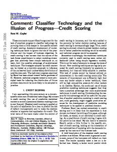
According to the distribution of good and bad applicants in Tables 3. and 4., the cut-off in LR models was estimated on the basis of distribution of goods and bads in the estimation sample.
10
Figure 1. Sampling procedure for two levels of experiments
RESULTS OF CREDIT SCORING MODELS Estimating probabilities for rejected credit applicants The first scoring model is used for the purpose of classifying the rejected credit applicants. NN results on the first level show that the best total hit rate of 76.3% is obtained by the backpropagation algorithm which also had the best hit rate for bad applicants (84.6%). Hit rates of the first scoring model for LR estimation gave the total hit rate of 83.08%, the good hit rate of 89.92% and the bad hit rate of 69.69%. Fitting measures such as Wald=45.6581 (p=0.0033); Score=77.3657 (p