Geoderma 318 (2018) 148–159
Contents lists available at ScienceDirect
Geoderma journal homepage: www.elsevier.com/locate/geoderma
Modeling soil organic carbon with Quantile Regression: Dissecting predictors' effects on carbon stocks
T
Luigi Lombardoa,b,*, Sergio Saiac, Calogero Schillacid, P. Martin Maib, Raphaël Husera a b c d
Computer, Electrical and Mathematical Sciences & Engineering Division, KAUST, Thuwal, Saudi Arabia Physical Sciences and Engineering Division, KAUST, Thuwal, Saudi Arabia Council for Agricultural Research and Economics (CREA), Research Centre for Cereal and Industrial Crops (CREA-CI), Foggia, Italy Department of Agricultural and Environmental Science, University of Milan, Italy
A R T I C L E I N F O
A B S T R A C T
Keywords: Quantile Regression R coding Topsoil organic carbon Digital soil mapping Mediterranean agro-ecosystem
Soil organic carbon (SOC) estimation is crucial to manage natural and anthropic ecosystems. Many modeling procedures have been tested in the literature, however, most of them do not provide information on predictors' behavior at specific sub-domains of the SOC stock. Here, we implement Quantile Regression (QR) to spatially predict the SOC stock and gain insight on the role of predictors (topographic and remotely sensed) at varying SOC stock (0–30cm depth) in the agricultural areas of an extremely variable semi-arid region (Sicily, Italy, around 25,000km2). QR produces robust performances (maximum quantile loss = 0.49) and allows to recognize dominant effects among the predictors at varying quantiles. In particular, clay mostly contributes to maintain SOC stock at lower quantiles whereas rainfall and temperature influences are constantly positive and negative, respectively. This information, currently lacking, confirms that QR can discern predictor influences on SOC stock at specific SOC sub-domains. The QR map generated at the median shows a Mean Absolute Error of 17 t SOC ha- 1 with respect to the data collected at sampling locations. Such MAE is lower than those of the Joint Research Centre at Global (18 t SOC ha- 1) and at European (24 t SOC ha- 1) scales and of the International Soil Reference and Information Centre (23 t SOC ha- 1) while higher than the MAE reached in Schillaci et al. (2017b) (Geoderma, 2017, issue 286, page 35–45) using the same dataset (15 t SOC ha- 1). The results suggest the use of QR as a comprehensive method to map SOC stock using legacy data in agro-ecosystems and to investigate SOC and inherited uncertainty with respect to specific subdomains. The R code scripted in this study for QR is included.
1. Introduction Soil Organic Carbon (SOC) plays a key role in various agricultural and ecological processes related to soil fertility, carbon cycle and soilatmosphere interactions including CO2 sequestration. Thus, its knowledge has a crucial importance both at global and local scales, especially when aiming at managing natural, anthropic areas and agricultural lands. In this context, the scientific community has spent considerable efforts in mapping SOC, its spatiotemporal variation, and in confirming its primary role in shaping ecosystems functioning (Ajami et al., 2016; Grinand et al., 2017; Ratnayake et al., 2014; Schillaci et al., 2017a). Spatio-temporal studies can be found in various geographic contexts from Africa (Akpa et al., 2016), Asia (Chen et al., 2016), Australia (Henderson et al., 2005), Europe (Yigini and Panagos, 2016), NorthAmerica (West and Wali, 2002), central America (Ross et al., 2013) to South-America (Araujo et al., 2016). The variability of the local landscape, availability of funding, mean gross income of the population in
*
the area, and temporal commitment affect the number of samples, their spatial density and distribution. As a result, experiments have been conducted on almost regular and dense grids, mostly focusing on small areas (Lacoste et al., 2014; Taghizadeh-Mehrjardi et al., 2016) and others using sampling strategies that significantly vary across space (Mondal et al., 2016). The latter studies mainly correspond to regional or larger scales (Reijneveld et al., 2009; Sreenivas et al., 2016), with only few cases having an optimal sample density maintained at a national level (Mulder et al., 2016). The characteristics of the environment under study can require the use of different predictors capable of explaining the variability of soil traits, topography and standing biocoenosis, especially (cropped or natural) phytocoenosis, the latter being efficiently explained by remotely sensed (RS) properties (Morellos et al., 2016; Peng et al., 2015). Modeling procedures for SOC primarily aim at constructing present, past or predictive maps, and at studying the role of each predictor over the target variable. Regarding the latter, the estimation of predictor
Corresponding author. E-mail address:
[email protected] (L. Lombardo).
https://doi.org/10.1016/j.geoderma.2017.12.011 Received 1 August 2017; Received in revised form 5 December 2017; Accepted 9 December 2017 0016-7061/ © 2017 Elsevier B.V. All rights reserved.
Geoderma 318 (2018) 148–159
L. Lombardo et al.
13°0'0"E
14°0'0"E
15°0'0"E
38°0'0"N
SOC stock
tonnes / hectare 0.0 - 9.7 9.7 - 14.1 14.1 - 17.6 17.6 - 20.9 20.9 - 24.0 24.0 - 26.5 26.5 - 29.8 29.8 - 32.3 32.3 - 35.2 35.2 - 37.6 37.6 - 40.1 40.1 - 42.2 42.2 - 44.8 44.8 - 48.6 48.6 - 52.5 52.5 - 57.8 57.8 - 67.9 67.9 - 89.9 89.9 - 242.6
37°0'0"N
0.95 ... Quantile Classification ... 0.05
37°0'0"N
38°0'0"N
12°0'0"E
0 12.5 25
12°0'0"E
50
13°0'0"E
75
100 km
14°0'0"E
15°0'0"E
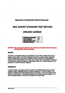
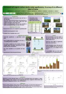
Fig. 1. SOC stock dataset and geographic contextualization.
SOC and SOC stock (Rodríguez-Lado and Martínez-Cortizas, 2015). However, they are bounded by definition to model the conditional mean, thus being unable to explore the effects of the same properties at different C contents or stock of the soil, especially near the tails of the distribution. In the present work, Quantile Regression (hereafter QR, Koenker (2005)) is used to model SOC stock from a non-homogenously sampled topsoil SOC dataset using soil texture, land use, topographic and remotely sensed covariates. In particular, QR is able to model the relationship between a set of covariates and specific percentiles of SOC stock. In classical regression approaches, the regression coefficients (also often called beta coefficients) represent the mean increase in the response variable produced by one unit increase in the associated covariates. Conversely, the beta coefficients obtained from QR represent the change in a specific quantile of the response variable produced by a one unit increase in the associated covariates. In this way, QR allows one to study how certain covariates affect median (quantile τ = 0.5) or extremely low (e.g., τ = 0.05) or high (e.g., τ = 0.95) SOC stock values. Therefore, it gives a more comprehensive description of the effect of predictors on the whole SOC stock probability distribution (i.e., not just the mean) and may be used to analyze differential SOC stock responses to environmental factors. Furthermore, when used for mapping purposes, QR allows for soil mapping at given quantiles, providing analogous estimates to more common approaches by using the median instead of the mean. A flexible non-parametric extension of linear QR, known as Quantile Regression Forest (QRF), was used in Malone et al. (2017) to derive conditional quantiles used to perform an efficient spatial downscaling. In the present experiment we use a nested strategy to model SOC stock in Sicilian agricultural areas with QR: we initially aim at testing the QR overall performances when modeling the SOC stock by segmenting its distribution into 19 quantiles (τ = 0.05 to τ = 0.95). Subsequently, we examine the coefficients of each predictor for each of the quantiles. Ultimately, we compare the median prediction with available SOC benchmarks for the same study area to test the efficiency of QR for soil mapping purposes. The dataset used in this contribution is the same used in Schillaci et al. (2017b) where a Stochastic Gradient Treeboost is adopted.
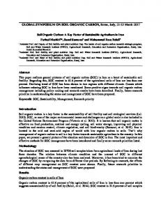
Fig. 2. Leave-one-out performance evaluation using the quantile loss.
contributions on a target variable such as SOC, is of particular interest to efficiently obtain agro-environmental and social benefits (e.g. Viscarra Rossel and Bouma, 2016). Statistical applications provide quantitative ways to deal with such research questions. The current literature encompasses algorithms that can be clustered into interpolative and predictive. Pure interpolators are broadly used when the density of the samples is sufficient to regularly describe the variation of SOC across a given area. Examples with excellent prediction performances are reported in Hoffmann et al. (2014), Piccini et al. (2014). The weakness of these approaches becomes evident when using datasets with non-regular distribution in space (Dai et al., 2014; Miller et al., 2016). Conversely, regressionbased predictive models hardly suffer from the spatial sampling scheme as they do not rely on the distribution across the geographic space in order to derive functional relations between SOC and independent variables (Hobley et al., 2016). Among these, linear regression models are a well-established tool for estimating how, on average, certain environmental properties affect 149
Geoderma 318 (2018) 148–159
L. Lombardo et al.
Fig. 3. Boxplots of estimated beta coefficients based on the simple model with 10,000 bootstrap replicates, and plotted with respect to the quantile level τ = 0.05,…,0.95. The blue line represents 0 (i.e., no effect), while the red curves are 95% pointwise confidence intervals.
2. Materials and methods
facilitates the decomposition and mineralization of the organic matter.
2.1. Study area
2.2. SOC data and predictors
Sicily with its approximately 25 thousand square kilometer area is the biggest Mediterranean island. More than 60% of its area is cultivated. The natural/semi-natural ecosystems include i) Mediterranean maquis, ii) dunes and coastal systems, iii) woods and forests. There are also 37 ancillary islands that were not considered in this study. Sicily has several sub-climatic zones, all of which are included in hot-summer Mediterranean climate (Csa Koeppen) and warm-summer Mediterranean climate (Csb Koeppen) with mean annual temperatures usually higher than 15.8° C. From the West to the South-East coasts, indicators of a semiarid environment can be observed over the year consisting of low or no rainfall summers, high air temperatures, evapotranspiration demand and water deficit. The mountainous areas (Madonie, Sicani, Nebrodi and Peloritani ridges, physiography can be checked in Schillaci et al. (2017a) and references therein) are scarcely cultivated mostly because of conservation policies in favor of the local temperate woodland. The continentality index, determined by the difference between the summer and the winter mean air temperature, is similar in all the climatic subregions. According to Fantappiè et al. (2010) using the World Reference Based (WRB, 2014) soil classification, the dominant soils in Sicily are: Entisols (36%), Inceptisols (34%), followed by the Mollisols, Alfisols, Vertisols and Andisols. This climatic context plays an important role on the decay processes of organic residue (Lützow et al., 2006) and on the stabilization of organic fractions. In particular, the local climatic setting
The available dataset represents the SOC stock (expressed in ton⋅ha) of the topsoils (Ap horizon, from 0 to 30 cm depth) primarily from agricultural areas (Fig. 1). It was calculated from the organic carbon (expressed in g⋅kg- 1) multiplied by the soil bulk density. The latter was derived by pedotransfer function (Pellegrini et al., 2007). In total, 2202 samples were used for modeling purposes; see Schillaci et al. (2017b) for further information on the dataset. Supplementary Fig. 1 illustrates the variability associated with each of the considered quantiles. The dataset was provided by the Assessorato Regionale Territorio Ambiente (ARTA) as georeferenced SOC values derived by pedological profiles and soil pits. The adopted covariates and their interpretation are discussed in the Supplementary Materials, Predictors Section. The distributions of the aforementioned covariates are shown in Supplementary Fig. 2 through their Empirical Cumulative Distribution Functions. Prior to any analysis, we transformed some of the variables. This is shown and explained in the Supplementary Material (Fig. 3 and Pre-processing Section, respectively). 1
2.3. Statistical modeling using linear quantile regression 2.3.1. Quantile regression In classical regression analysis, the fluctuations in the mean of a response variable (e.g., log(SOC)) are typically explained through a 150
Geoderma 318 (2018) 148–159
0.05
0.2
0.35
0.5
0.65
0.8
0.95
0.2
0.35
0.5
0.65
0.8
0.95
0.05
0.2
0.35
0.5
0.65
0.8
0.95
0.3
0.3 0.35
0.5
0.65
0.8
0.95
0.05
0.2
0.35
0.5
0.65
0.8
0.95
0.05
0.2
0.35
0.5
0.65
0.8
0.95
0.05
0.2
0.35
0.5
0.65
0.8
0.95
0.05
0.2
0.35
0.5
0.65
0.8
0.95
Quantile τ
Temperature
2 0
−0.2
−4
−2
Slope
0.2
0.1
−1000
0.1 −0.2
−0.1
0.0
Northness
Plan Curvature
0.2
0.6 0.4 0.2
NDVI
0.0 −0.2 −0.6 0.003 0.002 0.001 −0.001 0.000
Rainfall
0.05
0.05
1000
0.95
0.95
500
0.8
0.8
0
0.65
0.65
Profile Curvature
0.5
0.5
−500
0.35
0.35
1500
0.2
0.2
1000
0.05
0.05
500
0.95
0
0.8
−500
0.65
0.0
0.5
−0.1
0.35
0.1 −0.1 −0.2
0
0.2
0.8
0.05
0.0
Eastness
0.2
0.10 0.05 0.00
log(Catchment Area)
0.005 −0.010
0.000
Band8
400 300 200 100
Intercept
500
0.010
600
L. Lombardo et al.
Quantile τ
Quantile τ
Quantile τ
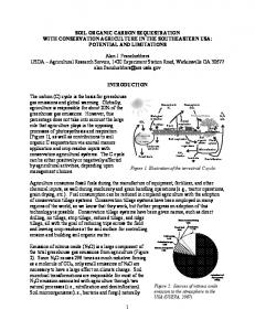
Fig. 4. Boxplots of estimated beta coefficients for continuous predictors. These results are based on the final model with 10,000 bootstrap replicates, and plotted with respect to the quantile level τ = 0.05,…,0.95. The blue line represents 0 (i.e., no effect), while the red curves are 95% pointwise confidence intervals.
predictor, focusing on a single feature (i.e., the mean) of the distribution of the response Y. More detailed information on the whole conditional (not necessarily Gaussian) distribution of the response Y may be obtained using quantile regression. By definition, for each probability 0 ≤ τ ≤ 1, the τ-quantile yτ of Y is the value exceeding (100 × τ)% of the data. Mathematically, one has pr(Y ≤ yτ) = τ, and the collection of all quantiles {yτ : 0 ≤ τ ≤ 1} fully characterizes the probability distribution of Y. The value τ = 0.5 corresponds to the median, while low and high quantiles (for low and high values of τ, respectively) correspond to extreme values of Y lying in the lower and upper tails of the distribution, respectively. By analogy with Eq. (1), the conditional τ-quantile may be estimated by minimizing an objective function, where the squared loss function is replaced by the quantile loss function. More precisely, computing
linear function of a set of predictors. In the case where n responses Y 1, …,Y n are observed with their p respective predictors x1i,…,xpi (assumed here to be continuous for simplicity), a statistical model may be formulated as
Yi = β0 + β1 x1i + ⋯+βp x pi + εi, where the random variables εi are typically assumed to be mutually independent and to follow a normal distribution with zero mean and finite variance σ2 > 0. Under such a model, when the predictors are linearly independent, the vector of unknown regression parameters β = (β1,…,βp) T may be estimated using the Ordinary Least Squares (OLS) estimator β(OLS ) , which may also be seen as minimizing the squared loss function, i.e.,
βOLS = (X T X )−1X T Y = min Y − Xβ
2
βτ = min
β
β
n
= min β
∑ (Yi − β0 − β1 x1i −⋯−βp xpi i=1
)2 ,
n
∑ Lτ (Yi − β0 − β1 x1i −⋯−βp xpi), i=1
(2)
where the quantile loss function Lτ is defined as
(1)
− 2(1 − τ ) x , L τ (x ) = ⎧ ⎨ ⎩ 2τx ,
where Y = (Y 1,…,Y n)T is the vector of observations, and X is the n-by(p + 1) design matrix. The first column corresponds to the intercept and is a vector of ones, and each other column corresponds to a specific predictor, i.e., it contains the values xk1,…,xkn, k = 1,…,p. From the right-hand side of Eq. (1), the conditional mean of Y may be estimated by β0; OLS + β1; OLS x1 + ⋯+βp; OLS x p . In other words, this is a point
x < 0; x ≥ 0,
the conditional τ-quantile yτ may then be estimated as ŷτ = β0; τ + β1; τ x1 + ⋯+βp; τ x p . When τ = 0.5, L0.5 = |x| is the absolute loss function, and ŷ0.5 corresponds to the estimated conditional median. In our application, we chose a sequence of 19 equispaced probabilities 151
Geoderma 318 (2018) 148–159
0.6 0.4 0.2 0.0 −0.4
0.95
0.5
0.65
0.8
0.95
0.05
0.2
0.35
0.5
0.65
0.8
0.95
1
0.8
0.35
0
0.65
0.2
−1
0.5
Quantile τ
0.05
−2
0.35
0.95
−3
0.2
Broad−leaved vegetation (311)
0.05
0.8
3
0.95
0.65
2
0.8
0.5
1
0.95
0.65
0.35
0
0.8
0.5
0.2
−1
0.65
0.35
0.05
−2
0.5
Quantile τ
−0.2
Olive Groves (223)
0.0 −1.0
0.35
0.2
1.0
0.2
0.05
0.5
0.05
0.95
Woodland−shrub (324)
Moors and heathland (322)
0.95
0.8
0.0
1.0 0.5 0.0 −0.5
Annual crops (241)
−1.0 1.0 0.5 0.0 −0.5
Natural grassland (321)
0.8
Mixed ecosystem (243)
0.95
0.65
0.65
−0.5
0.8
0.5
0.5
1.5
0.65
0.35
0.35
1.0
0.5
Quantile τ
0.2
0.2
0.5
0.35
0.05
0.05
0.0
0.2
0.95
Sclerophyllous vegetation (323)
0.05
0.8
−0.5
−0.2 0.95
0.65
0.6
0.8
0.5
0.4
0.65
0.35
0.2
0.5
0.2
0.0
0.35
0.05
−0.2
0.2
Complex cultivation (242) 0.05
−0.6
0.95
1.0
0.8
0.5
0.65
0.0
0.5
−0.5
0.35
−1.0
0.2
−1.5
0.05
−0.5
Fruit Trees (222)
0.6 0.4 0.2 0.0
Vineyards (221)
1.0 0.5 0.0 −0.5 −1.0
Urban Fabric (112)
0.5
L. Lombardo et al.
Quantile τ
Fig. 5. Boxplots of estimated beta coefficients for each category of Land Use. These results are based on the final model with 10,000 bootstrap replicates, and plotted with respect to the quantile level τ = 0.05,…,0.95. The blue line represents 0 (i.e., no effect), while the red curves are 95% pointwise confidence intervals. Numbers between parentheses correspond to the Corine 2000 codes. In particular, Mixed ecosystem corresponds to Land principally occupied by agriculture, with significant areas of natural vegetation (Corine 243).
τ = 0.05,0.1,…,0.95 to fit separate Quantile Regression models, giving much deeper insight into the complete conditional distribution of the SOC stock values, as a function of spatial predictors. By focusing on low (or high) quantiles, regression coefficients inform us about predictors that mainly influence the absence (or presence of high concentrations) of SOC stock over space. By considering independent Quantile Regression models for different values of τ, this allows for the possibility that the importance of certain predictors may change according to the SOC level. More statistical details on Quantile Regression and its application may be found in Koenker (2005). Finding the estimated parameters βτ by optimizing Eq. (2) is not trivial, but robust algorithms have been implemented and made freely available in the R package quantreg. Model checking and validation may be performed using classical regression techniques with some minor adjustments. For example, to assess the goodness of fit, the coefficient of determination R2 is typically replaced by a similar measure based on the quantile loss, although the interpretation remains essentially the same. Similarly, to check the ability of the model to predict unobserved values, cross-validation combined with the quantile loss function is typically used, in order to be consistent with the fitting procedure, instead of using the mean squared error as in classical regression analysis.
1. We perform a preliminary multicollinearity analysis to exclude highly correlated covariates. When Pearson's correlation coefficients are above 0.7 or below −0.7, we remove one of two or more collinear covariates as suggested by Pengelly and Maass (2001). This is shown and explained in the Supplementary Material (Fig. 4 and Preprocessing Section, respectively). 2. Categorical covariates are converted into dummy variables equivalent to each predictor level. Then, the most and least representative dummy classes are removed to avoid using a singular design matrix and subsequent parameter estimates. The least represented classes contain one to five SOC stock samples. This allows to remove potential sources of noise in the modeling procedure, whereas the effect of the most frequent class is carried in the model intercept. The most frequent classes account for a significant part of the data by definition, thus the interpretation of their contribution to the model is clearly important. To investigate their effects on SOC stock we pre-run a separate simpler model built only with the most frequent class within the covariates. 3. Model performances or predictive power is evaluated through leaveone-out cross-validation (Sammut and Webb, 2010). This allows for producing quality metrics based on the quantile loss (Koenker and Bassett Jr, 1978). 4. Model uncertainty over replicates is implemented through nonparametric case-resampling bootstrap (Davison and Hinkley, 1997). In particular, 10,000 replicates are generated by resampling each of
2.3.2. Model building strategy, estimation and uncertainty assessment The strategy adopted in the present work includes five steps: 152
Geoderma 318 (2018) 148–159
0.35
0.5
0.65
0.8
0.95
0.05
0.2
0.35
0.5
0.65
0.8
0.95
0.05
0.2
0.35
0.5
0.65
0.8
0.95
0.4 0.2 0.0
Loam
−0.2 −0.4 0.2
0.35
0.5
0.65
0.8
0.95
0.05
0.2
0.35
0.5
0.65
0.8
0.95
0.05
0.2
0.35
0.5
0.65
0.8
0.95
0.05
0.2
0.35
0.5
0.65
0.8
0.95
0.05
0.2
0.35
0.5
0.65
0.8
0.95
0.05
0.2
0.35
0.5
0.65
0.8
0.95
0.4 0.2 −0.2
−0.4
1 −2
−1
Sand
0
0.5 0.0
Loamy Sand Quantile τ
−4
−1.0
−3
−0.5
0 −1 −2 −3
Sandy Clay Loam
1.0
1
2
−0.2
0.0
Sandy Loam
0.4 0.2 0.0
Silty Clay Loam
0.6
0.8
1.0 0.8 0.6 0.4 0.2 0.0
Silty Loam
0.05
0.6
0.2
0.0
Silty Clay 0.05
−2.0 −1.5 −1.0 −0.5
0.2 −0.4
−0.2
0.0
Clay
0.4
0.5
0.6
1.0
0.6
0.8
L. Lombardo et al.
Quantile τ
Quantile τ
Fig. 6. Boxplots of estimated beta coefficients for each category of Texture. These results are based on the final model with 10,000 bootstrap replicates, and plotted with respect to the quantile level τ = 0.05,…,0.95. The blue line represents 0 (i.e., no effect), while the red curves are 95% pointwise confidence intervals.
Köchy (2011)) and iii) the European Joint Research Centre JRC European SOC map (Lugato et al., 2014). These layers represent the state of the art of digital soil mapping and are de facto the only SOC benchmarks for the globe and for Europe. According to Hengl et al. (2014), SOC distribution is calculated through Generalized Linear Models at a 1-km resolution using the GSIF package in R. Hiederer and Köchy (2011) use analogous linear regression model and spatial resolution to regionalize the SOC data over the globe. Conversely, the JRC European estimates are calculated using a deterministic approach using the agroecosystem SOC model CENTURY (Parton et al., 1988). Ultimately, we also extend the comparison to the SOC spatial prediction in Schillaci et al. (2017b) where the authors modeled the same data in the present contribution using a Stochastic Gradient Treeboost (SGT, hereafter) approach (details on the method can be found in Friedman (1999), Lombardo et al. (2015)). The reported spatial resolution is 100 m. The inclusion of such estimates in the present contribution allows to compare the regional QR prediction to reliable, robust and well tested analogous datasets. The comparison is based on the median QR prediction together with the aforementioned benchmarks. To accommodate for differences in the spatial resolution we downscale all maps to the minimum common resolution (1-km cell size) where the resulting values per pixel represent the average SOC stock among smaller pixels
the 2202 cases with replacement. As a result, 10,000 replicates of the beta coefficient estimates for each predictor and categorical class are produced for each of the 19 quantiles considered in this study. Similarly, 19 sets of 10,000 predictive maps are also computed. This procedure evaluates the variability of the modeling output and the reliability of the final estimates across replicates. 5. SOC regionalization is conducted by producing 19 distinct quantile predictive maps by using the original dataset without any resampling scheme to ensure the full predictive power for mapping purposes. The spatial resolution of these maps is 85 m, which corresponds to the coarsest resolution of the original gridded covariates with the exception of the climatic ones.
2.4. Currently available SOC estimations in the study area We consider four digital soil mapping products for the area under study, three of which correspond to global benchmarks and the last is the SOC stock map by Schillaci et al. (2017b). Their description is reported as follows: i) the ISRIC World Soil Information (http://www. isric.org, Hengl et al. (2014)), ii) the Global Soil Organic Carbon Estimates of the Harmonized World Soil Database (http://esdac.jrc.ec. europa.eu/content/global-soil-organic-carbon-estimates, Hiederer and 153
Geoderma 318 (2018) 148–159
0.95
0.05
0.2
0.35
0.5
0.65
0.8
0.95
0.35
0.5
0.65
0.8
0.95
0.05
0.2
0.35
0.5
0.65
0.8
0.95
0.05
0.2
0.35
0.5
0.65
0.8
0.95
0.05
0.2
0.35
0.5
0.65
0.8
0.95
1.0
High ridges
0.0 −0.5 −1.0 −2.0
−2.0
Midslope ridges
0.2
0.4 0.2
−1.5
0.5 0.0 −0.5
Quantile τ
0.0
Open slopes
−0.4 0.05
0.5
0.8
0.0
0.65
−1.0
0.5
−0.2
0.5 0.0 −1.0 0.35
0.5
0.2
−1.0
Upper slopes
−0.5
Valleys
0.5 0.0 −0.5 −1.0 0.05
1.0
Midslope Drainage
1.0
1.0
0.6
L. Lombardo et al.
Quantile τ
Quantile τ
Fig. 7. Boxplots of estimated beta coefficients for each category of Landform Classification. These results are based on the final model with 10,000 bootstrap replicates, and plotted with respect to the quantile level τ = 0.05,…,0.95. The blue line represents 0 (i.e., no effect), while the red curves are 95% pointwise confidence intervals.
range with τ < 0.15. Conversely, log(Catchment Area) and Mean Annual Rainfall effects to the prediction were always positive. Other predictors including Northness, Eastness have a positive effect on SOC stock whereas Slope the Slope effect is slightly negative at all quantiles, though not significant. In Fig. 5, Vineyards and Olive groves (Corine Code 221 and 223, respectively) showed a positive relationship with organic carbon content and a tendency for beta coefficients to decrease towards the upper quantiles. Conversely, coefficients of Land principally occupied by agriculture, with significant areas of natural vegetation~(Corine Code 243), Natural grassland (Corine Code 321) and Sclerophyllous vegetation (Corine Code 323) were positive but seemed to be constant with respect to the quantile level τ. The analogous representation for Texture is shown in Fig. 6. Here, the role of Texture emerged for few textural classes. In particular, Silty Loam, Silty Clay Loam, and Sandy Loam textures appear across all quantiles to be strongly, mildly, and weakly positive, respectively. The median beta coefficients per quantile in Clay and Sand showed an opposite pattern. On the one side, clay texture yielded very high positive beta coefficients at lower quantiles and decreased approximately to zero to the right tail of the SOC stock distribution. A similar, but less pronounced decrease in the beta coefficients is shown for the Silty Clay. Both Clay and Silty Clay present a very low internal variability, especially at the upper quantiles. On the other side of the spectrum, Sand texture seems to produce an increasing beta coefficient across the quantiles, from strongly negative in the left tail of the distribution to almost 0 near the right tail. However, associated variability of each quantile for Sand is very high, hindering its interpretation. Coefficients for Landform classes are summarized in Fig. 7 (except for Plains) where unexpectedly, none of the Landform classes appear to have a clear influence over the SOC stock in the study area and no clear pattern can be detected across quantiles. Predictive maps are shown in Fig. 8. As expected, they are increasing in terms of the quantile τ, and fully ordered (i.e., there is no quantile crossing at any spatial point). On the plotted scale, chosen to be common to all quantiles, variations in predicted SOC stock over the
in a given 1-km cell side. 3. Results Leave-one-out cross-validation performances appear in line with other methods in the literature. In particular, Schillaci et al. (2017b) reported an R2 of 0.47 whereas our quantile loss reached 0.49 for quantiles τ = 0.4,0.45 (see Fig. 2). In addition, Fig. 2 reveals that the quantile loss has a bell shape as a function of the quantile level. This implies that the predictive power decreases towards the tails of the distribution, as expected. The uncertainty of estimated beta coefficients (assessed by means of the non-parametric case-resampling bootstrap) is presented in five separate subplots: Fig. 3 presents boxplots of estimated parameters obtained from the 10,000 bootstrap replicates for the simple model comprising only three categorical variables. The estimated parameters for the final reference model are summarized in Figs. 4, 5, 6, and 7, which correspond to continuous predictors, Land use, Texture and Landform, respectively. The spatial prediction and its uncertainty are summarized in Figs. 8, 9 and 10. The simple model (see Fig. 3) accounts for the most represented categorical classes in Land use (Non-irrigated arables), Texture (Clay loam) and Landforms (Plains). This model is characterized by a very low intercept variability. Non-irrigated arables and Clay loam are negatively associated with SOC, and beta coefficients show a tendency to further decrease at the upper quantiles, especially for the textural class. Plains does not appear to be significant overall, and thus scarcely influences the SOC stock. Regarding the final more complex model, certain covariates appeared clearly significant, as shown through high deviations from the blue line corresponding to zero beta coefficient along the quantiles. This occurs particularly for the continuous covariates log(Catchment Area), Mean Annual Rainfall and Mean Annual Temperature as shown in Fig. 4. Mean Annual Temperature showed a negative effect at all quantiles < 0.15, although it is not significant in the lower quantile 154
13°0'0"E 14°0'0"E 15°0'0"E
13°0'0"E 14°0'0"E 15°0'0"E
Q05
Q15
Q05
Q15
190 1
0.7
Q35
Q25
Q35
Q45
Q55
Q45
Q55
Q65
Q75
Q65
Q75
Q85
Q95
Q85
Q95
13°0'0"E 14°0'0"E 15°0'0"E
13°0'0"E 14°0'0"E 15°0'0"E
13°0'0"E 14°0'0"E 15°0'0"E
13°0'0"E 14°0'0"E 15°0'0"E
37°0'0"N 37°0'0"N
38°0'0"N
38°0'0"N 37°0'0"N 38°0'0"N 37°0'0"N
37°0'0"N
37°0'0"N
38°0'0"N
38°0'0"N
37°0'0"N
Q25
38°0'0"N
262.5
38°0'0"N
37°0'0"N
Inter-Quartile SOC (t/ha)
SOC (t/ha)
37°0'0"N
38°0'0"N
37°0'0"N
13°0'0"E 14°0'0"E 15°0'0"E
38°0'0"N
13°0'0"E 14°0'0"E 15°0'0"E
38°0'0"N
Geoderma 318 (2018) 148–159
L. Lombardo et al.
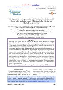
Fig. 8. Predictive maps (left side) together with their associated variability (right side). The latter is measured as the interquartile range, i.e., the distance between the 75% and the 25% quantiles, calculated from the 10,000 cross-validated maps. Grayed out regions correspond to no-data zones.
study area are evident in the extreme quantiles (τ≤ 0.25 and τ≥ 0.75) but seem less pronounced in the central quantiles (0.25 < τ < 0.75). Similarly, the variability (measured as inter-quartile range) showed an increasing trend through quantiles. A comparison between the predicted median (denoted Q50) and those of SGT (Schillaci et al., 2017b), ISRIC, European and Global JRC benchmarks is shown in Fig. 9. Among the available SOC Stock benchmarks, the SGT, JRC European maps and, to a certain degree, the ISRIC map are similar to our median map in term of degrees of spatial variability (Fig. 10). ISRIC frequently overestimates SOC stock in the study region. In particular, our predicted median and ISRIC maps effectively captured the pedo-genetic differences but not the differences within land use classes. JRC-EU better captured differences within arable lands, which was the most represented class of land use. Finally, JRC-GL captured few spatial differences but, together with our predicted median and SGT it captured the high SOC stocks in the southeastern areas. The MAE calculated with respect to the observed SOC stock data were MAE = 17 t SOC ha- 1 for the QR median, 15 t SOC ha- 1 for SGT, 24 t SOC ha- 1 for JRC European, 18 t SOC ha- 1 for the JRC Global, 23 t SOC ha- 1 for ISRIC. The spatial relation between predictive maps is compressed for a numerical-only assessment in Fig. 10. Here, the reference predicted median was compared to the four
benchmarks through i) pixel-by-pixel bivariate density scatterplots, ii) quantile-quantile plots, iii) empirical distributions of discrepancies between our predicted median and the benchmarks. Three observations can be made. SGT and ISRIC (even with a more pronounced deviation) overestimate the SOC stock compared to our median QR-based model, with similar values only at lower concentrations. The similarity between the median and the JRC-EU predictions is confirmed through the quantile-quantile plot showing a slight but constant underestimation. Ultimately, SGT and JRC-GL show the lowest discrepancy with respect to the QR median reference together with a good agreement up to a concentration of approximately 50 tha- 1. However, from this threshold to the right tail of the distribution, the two predictions do not agree.
4. Discussion We present a Quantile Regression framework for modeling the distribution of SOC stock data. This was applied to the semi-arid Sicilian territory located in the middle of the Mediterranean Sea. We explored its application by evaluating its predictive performance and by assessing it as a tool to provide a deeper information on predictor's effects at different carbon contents. This makes QR a valid tool to produce reliable soil maps at different quantile levels. A similar experiment is performed by Vaysse and Lagacherie (2017), where the 155
Geoderma 318 (2018) 148–159
L. Lombardo et al.
13°0'0"E
38°0'0"N
18
SGT
37°0'0"N
38°0'0"N
37°0'0"N
92
SOC (t/ha) 109 24
JRC EU
38°0'0"N 37°0'0"N
authors used Quantile Regression Forest (QRF) in a temperate Mediterranean area with a comparable SOC dataset in terms of areal extent, observation density and homogeneity of distribution. They report that QRF performs better than Regression Kriging in term of interpretation of uncertainty patterns and is better suited than other modeling methods when spatial sampling is sparse, such as in the present study. In terms of predictive skills, QR shows comparable results (maximum out-of-sample quantile loss of 0.49, in Fig. 2) to those obtained with Stochastic Gradient Treeboost (R2 of 0.47, Schillaci et al. (2017b)) using the same dataset, although comparison is difficult as the prediction target is not the same. Other experiments showed equivalent or worse performances. Yigini and Panagos (2016) obtained an R2 coefficient of 0.40 at the European scale with regression-kriging, whereas Meersmans et al. (2008) reported an R2 coefficient of 0.36 with multiple regression and Nussbaum et al. (2014) R2 of 0.35, both at regional scales. Here, the quantile loss highlighted a decreased performance near the left and right tails of the SOC stock distribution, as expected. The simple model intercept (Fig. 3) showed values bounded between 10 and 130 t/ha which are in line with the original dataset. Interestingly these values showed a very low variability. Such a low variability implies that the contributing effect of Non-irrigated arables, Clay loam, and, to a lesser extent, Plains is quite strong. Notably, the intercept of the final model (Fig. 4), that also bears the effects of the Non-irrigated arables, Clay loam and Plains, showed values very similar to the simple model but with a higher variability. This implies that the greater model complexity due to the inclusion of other predictors (both for continuous and categorical) can produce high ranges of variation in the SOC stock. This suggests that the uncertainty can be reduced by increasing the sample size. This information can be used to tailor the sampling strategy in a more efficient way. Mean Annual Rainfall and log(Catchment Area) coefficients were consistently positive, confirming the influence of soil moisture on carbon sequestration as reported in several articles (e.g., Saiz et al., 2012). These results partially disagree with Schillaci et al. (2017b), who found a scarce, but still positive, influence of the untransformed Catchment Area on SOC stock of the same area, with a method capable of handling non-Gaussian distributed data. In contrast with Mean Annual Rainfall and log(Catchment Area), Mean Annual Temperature showed negative and slightly varying beta coefficients across the whole SOC distribution. Recent surveys clearly highlighted the balance between temperature and rainfall in shaping the background SOC and SOC stock amounts and variations (Davidson et al. (2000), FAO (2017), Schillaci et al. (2017a)). However, the community continues to debate whether temperature has a positive correlation with SOC stocks (e.g., Conant et al., 2011, Wang et al., 2013, Sierra et al., 2015). In the present work, the strong negative effect of temperature supports the hypothesis that temperature negatively affects SOC accumulation in agricultural soils of Mediterranean areas even when SOC or rainfall (or both) is high. This could depend on the erraticness of precipitation and subsequent water availability as even at high rain discharges, part of the overland flow can be lost by runoff (Panagos et al., 2017). The ambiguous and low temperature effect and clear and positive rainfall effect at the lowest quantiles suggest that when SOC is low, managing water availability is more effective than temperature mitigation. Ultimately, Slope beta coefficients across quantiles were almost constantly negative confirming the influence of erosion on carbon stocks (Olson et al., 2016). From textural classes, a general positive influence emerged for mixed grain sizes. This is typical for Sicilian soils as sand classes do not have the capacity to fixate organic matter while pure clayey soils are extremely diverse. A peculiar effect characterized the Clay class with a positive beta coefficient from quantile 0.05 to 0.50 aligning to zero values from the median to the 95th percentile. This can be interpreted as a strong protective effect for small carbon contents up to a limit
SOC (t/ha)
SOC (t/ha) 78 9
JRC GL
38°0'0"N 37°0'0"N
15°0'0"E
Q50
SOC (t/ha) 124 20
ISRIC
38°0'0"N 37°0'0"N
14°0'0"E
SOC (t/ha) 214 27
Fig. 9. Available SOC-stock spatial-predictive maps in Sicily: Q50 corresponds to our median prediction, SGT represents the predictive results from Schillaci et al. (2017b), ISRIC is the SOC stock map from the International Soil Reference and Information Centre whereas JRC-EU and JRC-GL are the SOC stock benchmarks produced from the Joint Research Centre at the European and Global scale, respectively. Grayed out regions correspond to no-data zones where cultivation is either limited or absent.
156
Geoderma 318 (2018) 148–159
L. Lombardo et al.
Fig. 10. Bivariate comparison between our predicted median and available benchmarks. The first row shows a density scatterplot between our predicted median map and the four available benchmarks in each column. The second row presents the same information compressed in a quantile-quantile plot. The third row summarizes the distribution of discrepancies between our median predictions and the four benchmarks. Red dashed lines correspond to the diagonals with slope 1 (indicating a perfect match between the two predicted samples).
highlighted its contribution to SOC even in Mediterranean contexts (Mu noz-Rojas et al., 2013). In terms of soil mapping, the five maps (our median and the 4 benchmarks) agreed in depicting higher SOC stock levels around the Etna volcano and generally at the foothills. This may be interpreted as a result of particle transport where Carbon-rich soil from reliefs are eroded and deposited at the bottom of mountain ranges and/or different geological substrates producing soils with contrasting ability to retain organic C (Costantini and L’Abate, 2016; Mondal et al., 2016). A similar agreement was observed in the central portion of the study area, especially among Q50, SGT, and JRC-EU maps in lower SOC stocks, whereas JRC-GL and ISRIC benchmarks strongly deviated from Q50 for higher SOC contents. Conversely, the southeastern sector was shown to carry high SOC stocks for 4 maps with the exception of the European JRC benchmark, whereas the Global JRC one depicted less reasonable patterns and ISRIC overestimates the SOC stock with peaks well above any local measurement. Our Q50 SOC stock median map showed reasonable values similar to SGT and JRC and reasonable spatial patterns as ISRIC. This could be due to difference in resolution. ISRIC, Global and European JRC benchmarks are global or continental products and at such a scale the local landscape is often poorly represented. Here, QR was able to reach a good level of detail suggesting its use for different datasets and modeling scales.
where other factors need to interplay in order to further increase the carbon fixation/absorption (Badagliacca et al., 2017; Grimm et al., 2008; Mondal et al., 2016). Among different land uses strong positive relations can be recognized for Vineyards (Corine Code 221), Olive Groves (Corine Code 223), Land principally occupied by agriculture, with significant areas of natural vegetation (Corine Code 243), Natural Grassland (Corine Code 321) and Sclerophyllous vegetation (Corine Code 323). Vicente-Vicente et al. (2016) reported carbon sequestration rates of 0.78 tC ha- 1 yr- 1 Mediterranean vineyards. Similarly, Farina et al. (2017) suggested a potential SOC stock increase of 40.2% and 13.5% for vines and olives respectively, in similar environments to those considered in this study. In our work, such a positive effect was found also at the lowest boundary of the SOC distribution. This has a direct implication for land use management when aiming to increase SOC in such fragile ecosystems compared to arables. In Sicily, arables are mostly winter cereals and grain legumes, which respectively reduce N availability for the microorganisms and have few residues. Similarly, the positive effects of Land principally occupied by agriculture, with significant areas of natural vegetation (Corine Code 243) suggest that in-field and in-farm crop as well as landscape and environmental diversification can also favor SOC accumulation irrespective of the initial SOC levels in semi-arid Mediterranean environments, as also found in continental north-European areas by Kaczynski et al. (2017). Their work covers the time window between 1971 and 2013 during which the authors highlight a marked increase in SOC stock from 2001 coinciding with crop production as a very high yield provided very high input of carbon from crop residues. In environmental conditions differing from those in the present study, Tian et al. (2016) also showed that grassland quality, which depends on the diversification of its composition, has a determinant role on C sequestration rates. As regards the Sclerophyllous vegetation, other studies have
5. Conclusion Quantile Regression performs similarly to other statistical mapping methods and importantly, it enables considerations at various subdomains of the SOC stock distribution (Rudiyanto et al., 2016). Quantile Regression Forest, which transcends the linearity assumption by extending it to the more flexible non-parametric framework, has been shown to perform well with other datasets and contexts, and might 157
Geoderma 318 (2018) 148–159
L. Lombardo et al.
therefore yield even better performances in our case. This can be further explored in future research. The link between SOC stock amounts and the distribution of some Land Use classes (Vineyards (Corine Code 221), Olive orchards (Corine Code 223) and Mixed ecosystems (Corine Code 243)) or and presence of Clayey soils was positive and, above all, varying across the SOC distribution. This has direct implication in the management of agriculture at the regional level, since these crops are likely to contemporary increase the gross income of the area and also the ecosystem benefits, such as C sequestration in the soil. Variables like Vineyards or Clay change significantly through the SOC distribution. This suggests that classical linear regression methods may not recognize this trend and ultimately poorly represent the spatial variability of SOC at high or low carbon contents. Furthermore, advantages can be drawn from an agronomic point of view as a better understanding of environmental effects at various SOC concentrations can improve management schemes and allow for sequestration-tailored practices that preserve yield and rentability. This paper shows that Quantile Regression has valid and interesting agronomic applications for both in-field and landscape management, as also observed in few other examples (Casagrande et al., 2010; Van Zijl et al., 2014; Yu et al., 2016). To promote its application and reproducibility, the R code is made available in the Supplementary Materials.
stock variations in Italy during the last three decades. In: Land Degradation and Desertification: Assessment, Mitigation and Remediation. Springer, pp. 435–465. FAO, 2017. Food and Agriculture Organization of the United Nations, Rome, Italy. In: Global Symposium on Soil Organic Carbon. Farina, R., Marchetti, A., Francaviglia, R., Napoli, R., Di Bene, C., 2017. Modeling regional soil C stocks and CO2 emissions under Mediterranean cropping systems and soil types. Agric. Ecosyst. Environ. 238, 128–141. Friedman, J.H., 1999. Stochastic gradient boosting. Comput. Stat. Data Anal. 38, 367–378. Grimm, R., Behrens, T., Märker, M., Elsenbeer, H., 2008. Soil organic carbon concentrations and stocks on Barro Colorado Island - digital soil mapping using Random Forests analysis. Geoderma 146, 102–113. Grinand, C., Le Maire, G., Vieilledent, G., Razakamanarivo, H., Razafimbelo, T., Bernoux, M., 2017. Estimating temporal changes in soil carbon stocks at ecoregional scale in Madagascar using remote-sensing. Int. J. Appl. Earth Obs. Geoinf. 54, 1–14. Henderson, B.L., Bui, E.N., Moran, C.J., Simon, D., 2005. Australia-wide predictions of soil properties using decision trees. Geoderma 124, 383–398. Hengl, T., de Jesus, J.M., MacMillan, R.A., Batjes, N.H., Heuvelink, G.B., Ribeiro, E., Samuel-Rosa, A., Kempen, B., Leenaars, J.G., Walsh, M.G., Ruiperez Gonzalez, M., 2014. SoilGrids1kmglobal soil information based on automated mapping. PLoS One 9 e105992. Hiederer, R., Köchy, M., 2011. Global soil organic carbon estimates and the harmonized world soil database. EUR 79, 25225. Hobley, E.U., Baldock, J., Wilson, B., 2016. Environmental and human influences on organic carbon fractions down the soil profile. Agric. Ecosyst. Environ. 223, 152–166. Hoffmann, U., Hoffmann, T., Jurasinski, G., Glatzel, S., Kuhn, N., 2014. Assessing the spatial variability of soil organic carbon stocks in an Alpine setting (Grindelwald, Swiss Alps). Geoderma 232, 270–283. Kaczynski, R., Siebielec, G., Hanegraaf, M.C., Korevaar, H., 2017. Modelling soil carbon trends for agriculture development scenarios at regional level. Geoderma 286, 104–115. Koenker, R., 2005. Quantile Regression. Cambridge University Press. Koenker, R., Bassett Jr , G., 1978. Regression quantiles. Econometrica 46, 33–50. Lacoste, M., Minasny, B., McBratney, A., Michot, D., Viaud, V., Walter, C., 2014. High resolution 3D mapping of soil organic carbon in a heterogeneous agricultural landscape. Geoderma 213, 296–311. Lombardo, L., Cama, M., Conoscenti, C., Märker, M., Rotigliano, E., 2015. Binary logistic regression versus stochastic gradient boosted decision trees in assessing landslide susceptibility for multiple-occurring landslide events: application to the 2009 storm event in Messina (Sicily, southern Italy). Nat. Hazards 79, 1621–1648. Lugato, E., Panagos, P., Bampa, F., Jones, A., Montanarella, L., 2014. A new baseline of organic carbon stock in European agricultural soils using a modelling approach. Glob. Chang. Biol. 20, 313–326. Lützow, M. v., Kögel-Knabner, I., Ekschmitt, K., Matzner, E., Guggenberger, G., Marschner, B., Flessa, H., 2006. Stabilization of organic matter in temperate soils: mechanisms and their relevance under different soil conditions-a review. Eur. J. Soil Sci. 57, 426–445. Malone, B.P., Styc, Q., Minasny, B., McBratney, A.B., 2017. Digital soil mapping of soil carbon at the farm scale: a spatial downscaling approach in consideration of measured and uncertain data. Geoderma 290, 91–99. Meersmans, J., De Ridder, F., Canters, F., De Baets, S., Van Molle, M., 2008. A multiple regression approach to assess the spatial distribution of Soil Organic Carbon (SOC) at the regional scale (Flanders, Belgium). Geoderma 143, 1–13. Miller, B.A., Koszinski, S., Hierold, W., Rogasik, H., Schröder, B., Van Oost, K., Wehrhan, M., Sommer, M., 2016. Towards mapping soil carbon landscapes: issues of sampling scale and transferability. Soil Tillage Res. 156, 194–208. Mondal, A., Khare, D., Kundu, S., 2016. Impact assessment of climate change on future soil erosion and SOC loss. Nat. Hazards 82, 1515–1539. Morellos, A., Pantazi, X.-E., Moshou, D., Alexandridis, T., Whetton, R., Tziotzios, G., Wiebensohn, J., Bill, R., Mouazen, A.M., 2016. Machine learning based prediction of soil total nitrogen, organic carbon and moisture content by using VIS-NIR spectroscopy. Biosyst. Eng. 152, 104–116. Mulder, V., Lacoste, M., Richer-de Forges, A., Martin, M., Arrouays, D., 2016. National versus global modelling the 3D distribution of soil organic carbon in mainland France. Geoderma 263, 16–34. Mu noz-Rojas, M., Jordán, A., Zavala, L., González-Pe naloza, F., De la Rosa, D., PinoMejias, R., Anaya-Romero, M., 2013. Modelling soil organic carbon stocks in global change scenarios: a CarboSOIL application. Biogeosciences 10, 8253. Nussbaum, M., Papritz, A., Baltensweiler, A., Walthert, L., 2014. Estimating soil organic carbon stocks of Swiss forest soils by robust external-drift kriging. Geosci. Model Dev. 7, 1197–1210. Olson, K.R., Al-Kaisi, M., Lal, R., Cihacek, L., 2016. Impact of soil erosion on soil organic carbon stocks. J. Soil Water Conserv. 71, 61A–67A. Panagos, P., Ballabio, C., Meusburger, K., Spinoni, J., Alewell, C., Borrelli, P., 2017. Towards estimates of future rainfall erosivity in Europe based on REDES and WorldClim datasets. J. Hydrol. 548, 251–262. Parton, W.J., Stewart, J.W., Cole, C.V., 1988. Dynamics of C, N, P and S in grassland soils: a model. Biogeochemistry 5, 109–131. Pellegrini, S., Vignozzi, N., Costantini, E., L’Abate, G., 2007. A new pedotransfer function for estimating soil bulk density. In: Changing Soils in a Changing World: The Soils of Tomorrow. Book of abstracts. 5th International Congress of European Society for Soil Conservation, Palermo, pp. 25–30. Peng, Y., Xiong, X., Adhikari, K., Knadel, M., Grunwald, S., Greve, M.H., 2015. Modeling soil organic carbon at regional scale by combining multi-spectral images with laboratory spectra. PloS one 10 e0142295. Pengelly, B.C., Maass, B.L., 2001. Lablab purpureus (L.) Sweet-diversity, potential use and
Acknowledgment The authors are grateful to Maria Gabriella Matranga, Vito Ferraro and Fabio Guaitoli from the Regional Bureau for Agriculture, rural Development and Mediterranean Fishery, the Department of Agriculture, Service 7 UOS7.03 Geographical Information Systems, Cartography and Broadband Connection in Agriculture, Palermo. The authors would also thank Prof. Marco Acutis (University of Milan, Italy) for the stimulating discussions and MSc. Matthew Dimal (University of Twente, the Netherlands) for the final proofreading. Appendix A. Supplementary data Supplementary data to this article can be found online at https:// doi.org/10.1016/j.geoderma.2017.12.011. References Ajami, M., Heidari, A., Khormali, F., Gorji, M., Ayoubi, S., 2016. Environmental factors controlling soil organic carbon storage in loess soils of a subhumid region, northern Iran. Geoderma 281, 1–10. Akpa, S.I., Odeh, I.O., Bishop, T.F., Hartemink, A.E., Amapu, I.Y., 2016. Total soil organic carbon and carbon sequestration potential in Nigeria. Geoderma 271, 202–215. Araujo, J.K.S., de Souza Júnior, V.S., Marques, F.A., Voroney, P., da Silva Souza, R.A., 2016. Assessment of carbon storage under rainforests in Humic Hapludox along a climosequence extending from the Atlantic coast to the highlands of northeastern Brazil. Sci. Total Environ. 568, 339–349. Badagliacca, G., Ruisi, P., Rees, R.M., Saia, S., 2017. An assessment of factors controlling N2O and CO2 emissions from crop residues using different measurement approaches. Biol. Fertil. Soils. Casagrande, M., Makowski, D., Jeuffroy, M., Valantin-Morison, M., David, C., 2010. The benefits of using quantile regression for analysing the effect of weeds on organic winter wheat. Weed Res. 50, 199–208. Chen, L.-F., He, Z.-B., Zhu, X., Du, J., Yang, J.-J., Li, J., 2016. Impacts of afforestation on plant diversity, soil properties, and soil organic carbon storage in a semi-arid grassland of northwestern China. Catena 147, 300–307. Conant, R.T., Ryan, M.G., Ågren, G.I., Birge, H.E., Davidson, E.A., Eliasson, P.E., Evans, S.E., Frey, S.D., Giardina, C.P., Hopkins, F.M., et al., 2011. Temperature and soil organic matter decomposition rates-synthesis of current knowledge and a way forward. Glob. Chang. Biol. 17, 3392–3404. Costantini, E.A., L’Abate, G., 2016. Beyond the concept of dominant soil: preserving pedodiversity in upscaling soil maps. Geoderma 271, 243–253. Dai, F., Zhou, Q., Lv, Z., Wang, X., Liu, G., 2014. Spatial prediction of soil organic matter content integrating artificial neural network and ordinary kriging in Tibetan Plateau. Econ. Indic. 45, 184–194. Davidson, E.A., Trumbore, S.E., Amundson, R., 2000. Biogeochemistry: soil warming and organic carbon content. Nature 408, 789–790. Davison, A.C., Hinkley, D.V., 1997. Bootstrap Methods and their Application. Cambridge: Cambridge university press. Fantappiè, M., L’Abate, G., Costantini, E., 2010. Factors influencing soil organic carbon
158
Geoderma 318 (2018) 148–159
L. Lombardo et al.
temperature and moisture. J. Adv. Model. Earth Syst. 7, 335–356. Sreenivas, K., Dadhwal, V., Kumar, S., Harsha, G.S., Mitran, T., Sujatha, G., Suresh, G.J.R., Fyzee, M., Ravisankar, T., 2016. Digital mapping of soil organic and inorganic carbon status in India. Geoderma 269, 160–173. Taghizadeh-Mehrjardi, R., Nabiollahi, K., Kerry, R., 2016. Digital mapping of soil organic carbon at multiple depths using different data mining techniques in Baneh region, Iran. Geoderma 266, 98–110. Tian, Z., Wu, X., Dai, E., Zhao, D., 2016. SOC storage and potential of grasslands from 2000 to 2012 in central and eastern Inner Mongolia, China. J. Arid. Land 8, 364–374. Van Zijl, G.M., Ellis, F., Rozanov, A., 2014. Understanding the combined effect of soil properties on gully erosion using quantile regression. S. Afr. J. Plant Soil 31, 163–172. Vaysse, K., Lagacherie, P., 2017. Using quantile regression forest to estimate uncertainty of digital soil mapping products. Geoderma 291, 55–64. Vicente-Vicente, J.L., García-Ruiz, R., Francaviglia, R., Aguilera, E., Smith, P., 2016. Soil carbon sequestration rates under Mediterranean woody crops using recommended management practices: a meta-analysis. Agric. Ecosyst. Environ. 235, 204–214. Viscarra Rossel, R.A., Bouma, J., 2016. Soil sensing: a new paradigm for agriculture. Agric. Syst. 148, 71–74. Wang, G., Zhou, Y., Xu, X., Ruan, H., Wang, J., 2013. Temperature sensitivity of soil organic carbon mineralization along an elevation gradient in the Wuyi mountains, China. PloS One 8, 1–7. West, T.O., Wali, M.K., 2002. Modeling regional carbon dynamics and soil erosion in disturbed and rehabilitated ecosystems as affected by land use and climate. Water Air Soil Pollut. 138, 141–164. IUSS Working Group WRB, 2014. World reference base for soil resources 2014 international soil classification system for naming soils and creating legends for soil maps. FAO, Rome. Yigini, Y., Panagos, P., 2016. Assessment of soil organic carbon stocks under future climate and land cover changes in Europe. Sci. Total Environ. 557, 838–850. Yu, Y., Makowski, D., Stomph, T.J., van der Werf, W., 2016. Robust increases of land equivalent ratio with temporal niche differentiation: a meta-quantile regression. Agron. J. 108, 2269–2279.
determination of a core collection of this multi-purpose tropical legume. Genet. Resour. Crop. Evol. 48, 261–272. Piccini, C., Marchetti, A., Francaviglia, R., 2014. Estimation of soil organic matter by geostatistical methods: use of auxiliary information in agricultural and environmental assessment. Ecol. Indic. 36, 301–314. Ratnayake, R., Kugendren, T., Gnanavelrajah, N., 2014. Changes in soil carbon stocks under different agricultural management practices in North Sri Lanka. J. Natl. Sci. Found. 42. Reijneveld, A., van Wensem, J., Oenema, O., 2009. Soil organic carbon contents of agricultural land in the Netherlands between 1984 and 2004. Geoderma 152, 231–238. Rodríguez-Lado, L., Martínez-Cortizas, A., 2015. Modelling and mapping organic carbon content of topsoils in an Atlantic area of southwestern Europe (Galicia, NW-Spain). Geoderma 245, 65–73. Ross, C.W., Grunwald, S., Myers, D.B., 2013. Spatiotemporal modeling of soil organic carbon stocks across a subtropical region. Sci. Total Environ. 461, 149–157. Rudiyanto, Minasny, B., Setiawan, B.I., Arif, C., Saptomo, S.K., Chadirin, Y., 2016. Digital mapping for cost-effective and accurate prediction of the depth and carbon stocks in Indonesian peatlands. Geoderma 272, 20–31. Saiz, G., Bird, M.I., Domingues, T., Schrodt, F., Schwarz, M., Feldpausch, T.R., Veenendaal, E., Djagbletey, G., Hien, F., Compaore, H., et al., 2012. Variation in soil carbon stocks and their determinants across a precipitation gradient in West Africa. Glob. Chang. Biol. 18, 1670–1683. Leave-One-Out Cross-Validation. In: Sammut, C., Webb, G.I. (Eds.), Springer US, Boston, MA, pp. 600–601. Schillaci, C., Acutis, M., Lombardo, L., Lipani, A., Fantappiè, M., Märker, M., Saia, S., 2017a. Spatio-temporal topsoil organic carbon mapping of a semi-arid Mediterranean region: the role of land use, soil texture, topographic indices and the influence of remote sensing data to modelling. Sci. Total Environ. 601, 821–832. Schillaci, C., Lombardo, L., Saia, S., Fantappiè, M., Märker, M., Acutis, M., 2017b. Modelling the topsoil carbon stock of agricultural lands with the Stochastic Gradient Treeboost in a semi-arid Mediterranean region. Geoderma 286, 35–45. Sierra, C.A., Trumbore, S.E., Davidson, E.A., Vicca, S., Janssens, I., 2015. Sensitivity of decomposition rates of soil organic matter with respect to simultaneous changes in
159