modeling soil temperature, frost depth, and soil moisture redistribution ...

MODELING SOIL TEMPERATURE, FROST DEPTH, AND SOIL MOISTURE REDISTRIBUTION IN SEASONALLY FROZEN AGRICULTURAL SOILS F. C. Kahimba, R. Sri Ranjan, D. D. Mann ABSTRACT. Soil freezing and thawing processes and soil moisture redistribution play a critical role in the hydrology and microclimate of seasonally frozen agricultural soils. Accurate simulations of the depth and timing of frost and the redistribution of soil water are important for planning farm operations and choosing rotational crops. The Simultaneous Heat and Water (SHAW) model was used to predict soil temperature, frost depth, and soil moisture in agricultural soils near Carman, Manitoba. The model simulations were compared with three years of field data collected from summer 2005 to the summer 2007 in four cropping system treatments (oats with berseem clover cover crop, oats alone, canola, and fallow). The simulated soil temperatures compared well with the measured data in all the seasons (R 2=0.96‐0.99). The soil moisture simulations were better during the summer (RMSE=9.1‐12.0% of the mean) compared to the winter seasons (RMSE=17.5‐19.7% of the mean). During the winter, SHAW over‐predicted by 0.02 to 0.10 m 3 m ‐3 the amount of total soil moisture below the freeze front and under‐predicted by 0.02 to 0.05 m 3 m ‐3 the soil moisture in the upper frozen layers. The model was revised to account for the reduction in effective pore space resulting from frozen water to improve the winter soil moisture predictions. After this revision, the model performed well during the winter (RMSE=14.4% vs. 17.5%; R 2=0.74 vs. 0.67 in vegetated treatments, and RMSE=12.9% vs. 19.7%; R 2=0.73 vs. 0.52 in fallow treatments). The modified SHAW model is an enhanced tool for predicting the soil moisture status as a function of depth during spring thawing, and for assessing the availability of soil moisture at the beginning of the subsequent growing season. Keywords. SHAW model, Frost depth, Soil moisture, Soil freezing, Soil temperature.

S

oil freezing and thawing, soil temperature, and soil moisture redistribution affect the hydrology and microclimate of seasonally frozen agricultural soils. Freezing and thawing processes can influence soil moisture availability and redistribution during the fall through spring seasons (Kennedy and Sharratt, 1998; Flerchinger et al., 2006; Lin and McCool, 2006). Accurate simulation of the depth and timing of frost, soil temperature, and unfrozen and total soil water content is important for estimating the response of the soil to spring thawing and the soil moisture availability at the beginning of the subsequent growing season. Predicting soil moisture, frost depth, and soil temperature status during spring is important for planning early farm operations and for selecting suitable climate‐ and moisture‐sensitive crops (Bootsma and Brown, 1985; DeGaetano et al., 1996, 2000). However, the lack of

Submitted for review in May 2008 as manuscript number SW 7514; approved for publication by the Soil & Water Division of ASABE in July 2009. The authors are Frederick C. Kahimba, ASABE Member Engineer, former Research Fellow, Department of Biosystems Engineering, University of Manitoba, E2‐376 EITC Bldg, Winnipeg, MB, Canada (currently Lecturer, Department of Agricultural Engineering & Land Planning Sokoine University of Agriculture, Morogoro, Tanzania); Ramanathan Sri Ranjan, ASABE Member Engineer, Professor, and Daniel D. Mann, ASABE Member Engineer, Professor, Department of Biosystems Engineering, University of Manitoba, Winnipeg, MB, Canada. Corresponding author: R. Sri Ranjan, Department of Biosystems Engineering, University of Manitoba, E2‐376 EITC Bldg, Winnipeg, MB, R3T 5V6; phone: 204‐474‐9344; fax: 204‐474‐7512; e‐mail: [email protected].

field‐measured water content and soil temperature data and the complexity of the relevant hydrological processes are major difficulties in the validation of soil freeze‐thaw simulations (Kennedy and Sharratt, 1998; Warrach et al., 2001; Lin and McCool, 2006; Kahimba and Sri Ranjan, 2007). Advances in modeling technology have resulted in various models that deal specifically with soil freeze‐thaw phenomena. Examples are the SHAW model (Simultaneous Heat and Water) by Flerchinger and Saxton (1989a, 1989b), SOIL (simulation model for soil water movement and heat) by Jansson (1991), CLASS (Canadian Land Surface Scheme) by Verseghy et al. (1993), FROST (Kennedy and Sharratt, 1998), and SEWAB (Surface Energy and Water Balance) by Warrach et al. (2001). Many of these aforementioned models are sophisticated and are data intensive with long simulation times (Warrach et al., 2001). Other models such as SEWAB (Warrach et al., 2001) are less data intensive and have the advantage of faster execution times, but they tend to oversimplify the soil processes and produce less accurate simulations (Kennedy and Sharratt, 1998). In this article we used the physically based Simultaneous Heat And Water (SHAW) model to simulate soil temperature, duration and timing of frost, and soil moisture redistribution. The SHAW model was originally developed by Flerchinger and Saxton (1989a, 1989b) to simulate heat and water flow in the canopy‐snow‐surface‐soil system. Numerous studies have evaluated the ability of SHAW to predict evapotranspiration (Flerchinger et al., 1996), heat and water flow (Flerchinger et al., 2003), and within canopy surface radiation exchange (Flerchinger et al., 2006). Kennedy and

Applied Engineering in Agriculture Vol. 25(6): 871‐882

E 2009 American Society of Agricultural and Biological Engineers ISSN 0883-8542

871

Sharratt (1998) compared SHAW with SOIL, Benoit (1974), and Gusev (1985) models and concluded that the SHAW and SOIL better predicted frost depth. The limitations in the availability of continuous, simultaneously measured field data (specifically, unfrozen and total water contents, frost depths, and profile soil temperatures) has made it difficult in the past to extensively test model performance in agricultural soils experiencing seasonal soil freezing and thawing as occurs in central Canadian Prairies. Therefore, the objectives of this article were to: S Use SHAW model to simulate the depth and timing of frost, soil temperature, and soil moisture redistribution, S Compare SHAW output against measured field data for different seasons of the year, and S Improve SHAW's hydrologic process representations during soil freezing‐thawing to better predict soil moisture availability during winter and the subsequent growing season.

THE SHAW MODEL The SHAW model simulates heat, water, and solute transfer within a one‐dimensional soil profile through the plant canopy, snow, residue cover, and the soil (Flerchinger and Pierson, 1991; Flerchinger, 2000). Among important features of this model are the detailed accounting of snowmelt and soil freeze‐thaw processes and the simulation of transpiration and water vapor transfer through multi‐species plant canopies (Flerchinger and Saxton, 1989b). The model uses the energy balance approach to simulate frost depths. This approach is more accurate than the temperature‐driven approach in determining heat exchanges in the soil‐plant‐atmosphere ecosystem (Lin and McCool, 2006). The main equation in the model that accounts for the surface energy balance is (Flerchinger et al., 1996; Flerchinger, 2000): Rn + H + Lv E + G = 0

(1)

where Rn is net all‐wave solar radiation (W m‐2), H is sensible heat flux (W m‐2), Lv is latent heat of vaporization (J kg‐1), E is total evapotranspiration, Lv E is latent heat flux (W m‐2), and G is soil heat flux (W m‐2). The equation (eq. 1) describes the interrelation between the water fluxes and energy at the soil surface. The equation for soil water flux that takes into account the soil freezing and thawing is (Flerchinger, 2000): ∂θ l ρi ∂θ i ∂ ⎧ ⎛ ∂ψ ⎞⎫ 1 ∂qi + = ⎨K ⎢ + 1⎟⎬ + +U ∂t ρl ∂t ∂z ⎩ ⎝ ∂z ⎠⎭ ρl ∂z

(2)

where ql is volumetric liquid water content (m3 m‐3), qi is volumetric ice content (m3 m‐3), K is saturated hydraulic conductivity (m s‐1), t is time (s), z is soil depth (m), y is soil matric potential (m), and U is source/sink term (m3 m‐3 s‐1). The terms on the left side of equation 2 represent the change in volumetric liquid water content, and change in volumetric ice content, respectively. The terms on the right side represent the net liquid influx in a layer, net vapor influx, and

872

a source/sink term accounting for the water extraction by roots, respectively. All the terms are in m3 m‐3 s‐1. The unsaturated hydraulic conductivity (K) is a critical factor that determines the flow and redistribution of unfrozen water in unsaturated soils and in freezing soils. During the winter as soil begins to freeze, a small amount of free water become immobilized and does not participate in the flow. Hence the soil behaves as a drying soil with respect to liquid water availability and mobility. The unsaturated hydraulic conductivity (K) is calculated in the SHAW model using the following equation (Brooks and Corey, 1966): ⎛θ K = K S ⎢⎢ l ⎝ θS

⎛ 2⎞ ⎢ 3+ ⎟ b⎠

⎞⎝ ⎟ ⎟ ⎠

(3)

where Ks is saturated hydraulic conductivity (m s‐1), b is pore size distribution index, ql is the liquid soil water content at a given time (m3 m‐3 ), and qs is the saturated soil water content (m3 m‐3). The Brooks and Corey (1966) equation is used to relate the soil moisture characteristic as: ⎛θ ψ = ψ e ⎢⎢ l ⎝ θS

⎞ ⎟ ⎟ ⎠

−

1 b

(4)

where ye is air entry pressure (m) and y is soil matric potential (m). The main model assumption on the relationship between matric potential and unsaturated hydraulic conductivity is that frozen soils behave like unsaturated dry soils (Flerchinger, 1991, 2000). Hence the water flow in freezing soil will behave the same as water flow in drying soils. Therefore the soil moisture characteristic equation assumes that water flow behaves as in unsaturated soils. The detailed physics of various other components of the model have been described in Flerchinger and Saxton (1989a), Flerchinger and Pierson (1991), Flerchinger et al. (1996), and Flerchinger (2000). Since its development in 1989 and subsequent improvements, SHAW has been verified and used by many other researchers to simulate heat, water, and solute transfer within the soil/plant/atmosphere ecosystem (e.g. Kennedy and Sharratt, 1998; DeGaetano et al., 2000; Flerchinger et al., 1996, 2003, 2006). Flerchinger et al. (2006) improved a previous weakness that over‐predicted mid‐day canopy temperatures due to simplified assumptions of long‐wave radiation transfer within the canopy (Flerchinger et al., 2006). Other improvements include simulation of the depth and timing of frost (Kennedy and Sharratt, 1998; DeGaetano et al., 2000). Sensitivity analyses have indicated that air temperature, initial snow depth, and lower boundary soil temperature values have a larger influence on frost depth than soil hydraulic parameters (Flerchinger, 1991). The limited availability of soil moisture, depth and timing of frost, and soil temperature data measured in the winter have hindered extensive verification of various components of the SHAW model simulations (e.g. Flerchinger et al., 1996; Xiao et al., 2006). The field data on soil profile temperature, the unfrozen and total water contents presented in the current

APPLIED ENGINEERING IN AGRICULTURE

study will enhance model evaluation in this and similar regions experiencing seasonal soil freezing and thawing.

MATERIALS AND METHODS DESCRIPTION OF THE STUDY SITE The study site was at the Ian N. Morrison Research Farm of the University of Manitoba located in Carman, Manitoba (49° 30' N, 98° 02' W, 262‐m elevation above m.s.l). The area experiences seasonal soil freezing with 119 to 126 frost‐free days starting from 15 May to 26 September (Environment Canada, 2007; Nadler, 2007). The average annual (15‐year average, 1991‐2005) precipitation and temperature are 588.8 mm and 3.4°C, respectively (Environment Canada, 2007). The maximum monthly mean temperature occurs in July (+19.1°C), while the minimum (‐16.2°C) occurs in January (Kahimba et al., 2008). The experimental farm has a relatively flat topography with ground slopes ranging from 0.0 to 0.5%. The soil at the experimental site is classified as a well‐drained Hibson, with a texture class of very fine sandy loam from the sub group Orthic Black Chernozem (Mills and Haluschak, 1993) or Mollisol (very fine sandy loam) in the USDA Soil Taxonomy. The soil profile is relatively uniform with the depth to clay layer ranging between 0.70 and 0.75 m (Mills and Haluschak, 1993). The experimental site was located within a long‐term no‐till, 4‐year crop rotation trial which was started in year 2000 (Kahimba et al., 2008). This rotation consisted of six different cropping systems as treatments of which only four treatments (oats with berseem clover cover crop, oats alone, canola, and fallow) were chosen for this study. INSTRUMENTATION AND FIELD DATA COLLECTION Simulating the winter‐time movement of unfrozen water in frozen soil is a challenge for many soil moisture models for many reasons, but the difficulty of obtaining both frozen and unfrozen soil water data throughout the year is especially challenging for model validation. Most soil moisture measurement techniques can measure either the total soil water content [e.g. Neutron Moisture Meter (NMM) and gravimetric] or the unfrozen water content [e.g. Time Domain Reflectometry (TDR)] but not both water phases simultaneously. In addition, data collection in agricultural experiments is largely confined to the growing season, not during frozen conditions. In this study, the unfrozen water content for different soil depths was measured using the TDR method at 0.1‐m depth and at 0.2‐m intervals from 0.2 to 0.8 m. The total water content was measured using the NMM technique at 0.2‐m intervals from 0.2 to 1.8 m. The TDR method is regarded as the most practical technique for measuring liquid water content in frozen soils (Seyfried and Murdock, 1996). Both techniques were used on the same day within approximately 2 h on each date of data collection. The soil temperature was also measured on the same day, at the same depths of TDR measurement using digital thermocouple thermometer with a precision of ±0.1°C. The soil moisture and soil temperature data collected from the field were used for comparison with SHAW model simulations.

Vol. 25(6): 871‐882

MODEL INPUT PARAMETERS The SHAW model is a physically‐based model that has extensive data requirements. It requires initial conditions of soil temperature and soil moisture profiles at each soil depth (node) and the depth of snow at the start of simulation. Other model input parameters are the general site information, weather conditions, and soil and plant parameters. The hourly weather data used in the simulation were collected from the automatic weather station located within the Research Farm, about 300 m from the selected experimental treatment plots. Tables 1 and 2 give soil and plant input parameters, respectively, used in this simulation. Detailed descriptions of the model input parameters are presented in Flerchinger and Saxton (1989a, 1989b) and Flerchinger (2000). The solar radiation data obtained from the automatic weather station were available only during the growing season from April to September. For the period between September and April, solar radiation was estimated using the SolarCalc model developed by Spokas and Forcella (2006). SolarCalc uses daily maximum and minimum air temperatures (°C) and total precipitation (mm) as inputs. The model also requires inputs of simulation year and the topographic characteristics of the area (latitude, longitude and elevation above m.s.l). The output from the SolarCalc model is hourly incoming solar radiation (W m‐2). Soil temperature data were measured at 0.1‐, 0.2‐, 0.4‐, 0.6‐, and 0.8‐m soil depths. The soil temperatures at depths below 0.8 m were interpolated between 0.8 and 4.0 m assuming that Table 1. Soil characteristics used as input parameters for the SHAW model. Soil Depth Range (m) Soil Characteristic

0.0‐0.2 0.2‐0.4 0.4‐0.6 0.6‐0.8 >0.8

Particle size distribution (%) Sand Silt Clay Organic matter Campbell's pore size distribution index

79.00 8.00 13.00 3.76 3.05

73.00 8.00 19.00 2.72 3.22

77.00 7.00 16.00 1.24 3.18

77.00 4.00 7.00 44.00 16.00 52.00 1.24 0.00 3.12 3.05

Air entry potential (m) ‐0.4 Saturated hydraulic conductivity 2.90 (cm/h)

‐0.22 4.58

‐0.21 4.00

‐0.20 ‐0.20 0.41 0.2

Bulk density (kg/m3)

1420

1400

1400

1250

1310

Table 2. Plant characteristics used as input parameters for the SHAW model. Farm Management Year 2005‐2006

Year 2006‐2007

Oats with Berseem Clover

Oats Alone

Canola

Height of plant species (m) Width of plant leaves (cm) Dry biomass of plant species (kg/m3)

1.00 2.50 0.67

1.00 2.50 0.74

1.20 10.00 0.60

Leaf area index (LAI) Effective rooting depth (m)

3.10 0.75

3.10 0.75

3.3 0.95

Plant Characteristic

873

the temperature at 4.0‐m depth was equal to the average annual air temperature of 3.4°C (Flerchinger et al., 1996; Environment Canada, 2007). The SHAW model also requires the initial surface soil temperature at the initial hour of simulation as an input variable at the surface node. However, in this study no probes were installed at the surface to measure the soil temperature. Hence, a procedure developed by Gupta et al. (1990) was adopted for estimating the surface soil temperature. In their study, Gupta et al. (1990) stated that the daily maximum and minimum air temperature measured at 2.0‐m height is directly proportional to the upper boundary soil temperature, depending on soil surface conditions. The hourly soil surface temperature was estimated using the normalized hourly values and the maximum and minimum soil surface temperature as (Gupta et al., 1990): Tot = Γot (To max − To min ) + To min

(5)

where Tot is the estimated soil surface temperature at time (t), Got is the average normalized hourly soil surface temperature, Tomax is the estimated maximum soil surface temperature, and Tomin is the estimated minimum soil surface temperature. Hence using the proposed procedure, the daily maximum and minimum air temperature obtained from the weather station were used to estimate the daily maximum and minimum soil surface temperatures that were further used to estimate the hourly soil surface temperature at depth 0.0 m and time t. Details on the procedure for estimating the hourly soil temperatures at various soil depths and for different soil surface conditions are explained in Gupta et al. (1984, 1990). THE SHAW MODEL SIMULATIONS The SHAW model was used to predict the soil temperature, depth and timing of frost, and the unfrozen and total water contents from the summer of 2005 to the summer of 2007. The model performance was assessed in the following four cropping systems: 1) oats with berseem clover cover crop, 2) and oats alone (2005‐2006 season), 3) canola (2006‐2007), and 4) continuous fallow. The model was also used to simulate the depth and timing of frost and the accumulation of snow during the winter. The performance of SHAW was evaluated in the summer and fall when the soil was unfrozen, and in the winter when the soil was at least partially frozen. The ground cover effect was also evaluated for the two seasons. The predicted values of total soil water content, the profile soil temperature, and frost depth were compared with the measured values. Based on the simulations of the model for different seasons of the year, aspects of the model needing improvement were identified. Revised equations were developed to improve model predictions to better simulate the soil water and temperature during the winter when the soils were partly frozen and soil moisture exists in both frozen and unfrozen states. The model was also used to assess the soil response to fall freeze‐up and spring snowmelt under different farm management practices and to determine the soil moisture status at the beginning of the next growing season. STATISTICAL MODEL VALIDATIONS Various statistical analyses, including absolute and relative error measures (Willmott et al., 1985), were used to assess model performance. Both the square of thePearson's product‐moment correlation coefficient (r2) and the

874

coefficient of determination (R2) were used to measure the correlation between the measured and the predicted water content and soil temperature. The R2 values range between 0.0 and 1.0 with values close to 1.0 indicating better correlation (Spokas and Forcella, 2006). It can be oversensitive to extreme values and cannot detect the additive and proportional differences between the Pi and Mi (Willmott et al. 1985). Hence, higher values of R2 may not necessarily mean better model performance (Willmott et al., 1985; Spokas and Forcella, 2006). The R2 was calculated as (Legates and McCabe Jr., 1999): ⎡ ⎪ R2 = ⎪ ⎪ ⎪⎣

∑in=1 ( M i

[∑

n i =1 ( M i

− M ) ( Pi − P )

][∑

− M )2

n i =1 ( Pi

− P )2

]

⎤ ⎥ ⎥ ⎥ ⎥ ⎦

2

(6)

where Mi and Pi are the measured and predicted values, respectively; n is the total number of observations; and M and P are the means of the measured and predicted values, respectively. The index of agreement (d) also measures the correlation between the measured and simulated values and considers the differences between means and variances of Pi and Mi. The value of d ranges between 0.0 and 1.0, with values close to 1.0 indicating better model agreement ( Spokas and Forcella, 2006). It was calculated as: ⎡ ⎪ d = 1.0 − ⎪ ⎪ ⎪ ⎪⎣

∑in=1 ( M i

− Pi )

2

∑in=1 ( Pi − M + M i − M

)2

⎤ ⎥ ⎥ ⎥ ⎥ ⎥⎦

(7)

where Mi and Pi are the measured and predicted values, respectively; n is the total number of observations; and M and P are the means of the measured and predicted values, respectively. While the R2 and d indicate the degree of agreement between measured and predicted values, they do not account for proportional differences in measured and the predicted values and thus can easily be biased by extreme values (Willmott et al., 1985; Legates and McCabe Jr., 1999). Hence, the relative error measures should be supplemented with absolute error measures (Spokas and Forcella, 2006). Considering the absolute error measures, the root mean square error (RMSE) was calculated as (Legates and McCabe Jr., 1999): RMSE =

1 n ∑ ( M i − Pi ) 2 n i =1

(8)

where n is the number of observations, Mi is the measured, and Pi is the predicted soil moisture. When expressed as a percentage of the mean, a RMSE (%) value of 10 is regarded as a reasonable accuracy for most agricultural experiments (Tarpley, 1979). The mean absolute error (MAE) gives the weighted average of the absolute value of errors. A better model performance is when the MAE is close to zero. The MAE was calculated as (Legates and McCabe Jr., 1999):


(9)

where variables in equation 9 have the same definitions as in equation 8. The mean bias error (MBE) gives the uniformity of errors distribution. It assists in determining whether the model is overestimating or underestimating the measured values. A value close to zero indicates that the errors are evenly distributed, while a negative value of Pi - Mi indicates under‐estimation. The MBE was calculated as: 1 n

n

∑ ( Pi − M i )

(10)

i =1

where variables in equation 10 have the same definitions as in equation 8. The absolute error measures have the advantage that they are not influenced by outliers, and they take into account the proportional and additive differences between the measured and the predicted values (Legates and McCabe Jr., 1999). They also give a better indication of model accuracy since they can be expressed in the same units of the measured data (Tarpley, 1979).

Total water content (m 3 m-3)


0.0 0.1 0.2 0.3 0.4 0.5 0.6

0.0 0.1 0.2 0.3 0.4 0.5 0.6

0.0

0.0

0.4

(a)

0.8

DOY 347 2005

1.2 Measured WC Pred WC

1.6

RESULTS AND DISCUSSIONS

2.0

(b)

0.8

DOY 355 2005


2.0



0.0 0.1 0.2 0.3 0.4 0.5 0.6

0.0

0.0

Soil depth (m)

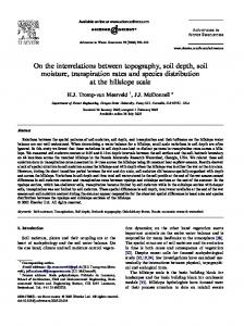
SOIL MOISTURE SIMULATION ON DIFFERENT CROPPING SYSTEMS The SHAW model was used to predict soil moisture in vertical soil profiles at depths from 0.0 to 1.8 m for different cropping systems from the summer of 2005 to the summer of 2007. On average, the model performed better in the vegetated treatments than in the continuous fallow treatment (table 3). The variation with depth of the simulated and measured total soil moisture from 0.0‐ to 1.8‐m soil depth on the vegetated treatment (oats with berseem clover) for the 2005 season is presented in figure 1. At the end of winter, in late March 2006, the measured frost depth was 0.6 to 0.7 m for the vegetated treatment and 0.8 to 1.0 m for the fallow. During February and March 2006, the model over‐predicted the total soil moisture just below the freeze front by 0.02 to

0.4

1.6

0.1

0.2

0.3

0.4

0.5

0.0

Soil depth (m)

MBE =

0.05 m3 m‐3 and under‐predicted the total soil moisture above the freeze front by 0.01 to 0.04 m3 m‐3 (fig. 1c, 1d). The model simulated the soil moisture fairly well during all the seasons in the unfrozen layers below 1.2 m. For the continuous fallow treatment (fig. 2), SHAW over‐predicted the freeze front at 0.8‐m soil depth and under‐predicted it in the top 0.5 m. Kahimba et al. (2008) presented the soil freezing patterns indicating that the depth of freeze front could be indicated by the region of zero soil moisture measured by TDR, which aligns with the lowest total soil moisture measured by NMM. In this case the freeze front in the fallow was about 0.8 m deep by 29 March 2006 [day of year (DOY) 88] (fig. 2). The model over‐predicted the total soil moisture below the freeze front by 0.04 to 0.11 m3 m‐3 in the fallow treatment. The over‐prediction below the freeze front in winter months indicated that the model

Soil depth (m)

⎤ 1 ⎡n ⎪∑ M i − Pi ⎥ n ⎣i =1 ⎦

Soil depth (m)

MAE =

0.4

(c)

0.8

DOY 55 2006

1.2

0.4

(d)

0.8

DOY 88 2006

1.2

1.6

1.6

2.0

2.0

Figure 1. Measured and predicted total soil water contents at different soil depths in the oats + berseem clover cover crop during: (a) the fall on 13 Dec. 2005, (b) early winter on 21 Dec. 2005, (c) late winter on 24 Feb. 2006, and (d) early spring on 29 March 2006. The measured water contents (WC) were taken using NMM method.

Table 3. The SHAW model statistical analysis for the measured and predicted total soil moisture and soil temperature during the 2005‐2007 seasons. Statistical Parameters Absolute Error Measures[b] Year

Farm Management

N

R2

d

MAE

MBE

ME

RMSE

RMSE (%)

Total soil moisture

Oats+berseem Oats alone Fallow

77 97 98

0.90 0.66 0.74

0.99 0.87 0.93

0.02 0.04 0.04

0.00 ‐0.03 ‐0.01

0.07 0.09 0.09

0.03 0.05 0.05

8.82 14.11 11.91

Soil temperature

Oats+berseem Oats alone Fallow

72 91 88

0.96 0.96 0.96

0.98 0.98 0.99

0.49 0.55 0.34

‐0.45 ‐0.55 ‐0.01

1.8 1.7 2.1

0.65 0.73 0.58

31.65 42.60 36.41

Total soil moisture

Canola Fallow

107 107

0.76 0.63

0.91 0.86

0.04 0.05

‐0.02 ‐0.03

0.12 0.11

0.06 0.06

19.54 18.35

Soil temperature

Canola Fallow

106 110

0.99 0.99

1.00 1.00

0.80 0.80

‐0.76 ‐0.32

4.3 4.8

1.20 1.28

14.00 13.12

Parameter

2005/2006

2006/2007

[a] [b]

Relative Error

Measures[a]

The parameters are: N = number of observations, R2 = coefficient of determination, d = index of agreement. The parameters are: MAE = mean absolute error, MBE = mean bias error, ME = maximum error, RMSE = root mean square error.

Vol. 25(6): 871‐882

875

Total water content (m3 m-3)

Total water content (m3 m-3) 0.2

0.3

0.4

0.0

0.5

0.8

Soil depth (m)

Soil depth (m)

0.4

0.1 0.2 0.3 0.4

0.5

0.0

(a) DOY55 2006


1.6

0.4 0.8

(b) DOY88 2006

1.2 1.6

2.0

2.0

Figure 2. Measured and predicted total soil water contents at different soil depths in the fallow during: (a) winter on 24 Feb. 2006 and early spring on 29 March 2006. The measured water contents (WC) were taken using NMM method.

allowed less soil moisture migration from below the freeze front towards the frozen soil layer as the freeze front advanced downward. The reduced upward migration was also a cause for the decreased simulated total water content in the frozen soil layers above the freeze front. SOIL TEMPERATURE SIMULATION IN DIFFERENT CROPPING SYSTEMS Model simulation of soil temperature was also evaluated on different cropping systems. The model performed well on all the cropping systems during the two simulation years. The R2 ranged between 0.96 and 0.99 on both the vegetated and fallow treatments (table 3). The mean absolute error ranges were 0.5°C‐0.8°C and 0.3°C‐0.8°C for the vegetated treatments and the continuous fallow, respectively (table 3). The MBE ranged between ‐0.45°C and ‐0.76°C for the vegetated treatments and between ‐0.01°C and ‐0.32°C for the fallow. The negative values of MBE indicated that on average the SHAW model slightly under‐estimated the actual Soil temperature (oC) -5.0 -2.5 0.0 2.5 5.0 7.5

Soil temperature (oC) -5.0 -2.5 0.0 2.5 5.0 7.5

0.4

DOY 347 2005

0.8 1.2 Meas tmp Pred tmp

1.6 2.0

Soil temperature (oC) -5.0 -2.5 0.0 2.5 5.0

1.6 2.0

DOY 347 2005

0.4

DOY 88 2006

0.8 1.2 1.6

Meas tmp

2.0

Pred tmp

0.4

(a3)

0.8

DOY 94 2006

1.2

0.4

(b2)

0.8

DOY 88 2006

1.2 1.6 2.0

Meas tmp Pred tmp

1.6 2.0

Soil temperature (oC)

Soill depth (m)

Soill depth (m)

1.2

(b1)

0.0 (a2)

-5.0 -2.5 0.0 0.0

0.0

0.8

Soil temperature (oC) -5.0 -2.5 0.0 2.5 5.0 7.5

0.0 (a1)

Soill depth (m)

Soill depth (m)

0.0

0.4

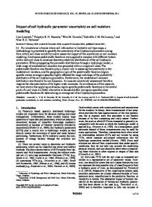
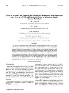
COMPARISON OF SUMMER AND WINTER MODEL SIMULATIONS Soil Moisture Simulations The accuracy of SHAW simulations of soil moisture was better in the summer when the soil was unfrozen than in winter when the soil was frozen (table 4). Based on the RMSE value of 10% (Tarpley, 1979), the model performed fairly well during the summer but not as well during the winter. In their study, DeGaetano et al. (1996) also noted that the presence of vegetation and crop residue increases the complexity of the winter soil freezing and thawing processes. The seasonal model accuracy of soil moisture predictions also varied depending on the ground cover condition (fig. 4). Results indicated that during the summer, better model performance was observed in the fallow compared to the vegetated treatments (fig. 4 a1 and b1; table 4). The difference between the vegetated and fallow treatments in the summer model simulations could be associated with the uncertainties in estimation of plant physical parameters and growth performance such as the measurements of leaf area index, plants biomass, and root lengths on the vegetated treatments. The continuous fallow treatment was poorly simulated during the winter compared to vegetated treatments (table 4; figs. 4 a2, b2). In summary, SHAW better simulated soil moisture during the summer than winter regardless of ground

Soill depth (m)

0.1

2.5

Soil temperature (oC)

5.0

-5.0 -2.5 0.0 0.0 Soill depth (m)

0.0 0.0

profile soil temperature on both vegetated and fallow treatments (table 3 and fig. 3). Figure 3 presents the variation with depth of the simulated and measured profile soil temperature from 0.0‐ to 1.8‐m soil depth for the vegetated (oats with berseem clover) and continuous fallow treatments. Ground cover conditions did not affect the accuracy of the model in simulating the soil temperature at different soil depths.

0.4

(b3)

0.8

DOY 94 2006

2.5

5.0

1.2 1.6 2.0

Figure 3. Measured and predicted soil temperature at different soil depths (a) in the oats + berseem clover cover crop, and (b) in the fallow. The (a1) and (b1) measurements were during the fall, (a2) and (b2) during winter, and (a3) and (b3) during spring.

876


Table 4. Comparison of the summer and winter SHAW model predictions of soil moisture and soil temperature on vegetated and continuous fallow treatments in the 2005‐2007 seasons. Statistical Parameters Absolute Error Measures[b] Farm Management

Vegetated treatment

Continuous fallow treatment

Parameter

Season of Simulation

N

R2

d

MAE

MBE

ME

RMSE

RMSE (%)

Total soil moisture

Summer Winter

118 116

0.90 0.67

0.97 0.89

0.02 0.04

‐0.02 ‐0.02

0.08 0.16

0.04 0.06

12.01 17.54

Soil temperature

Summer Winter

113 110

0.99 0.91

1.00 0.90

0.50 0.66

‐0.44 ‐0.66

2.5 2.1

0.80 0.82

8.68 73.00

Total soil moisture

Summer Winter

64 109

0.92 0.52

0.97 0.84

0.02 0.05

‐0.02 0.00

0.07 0.20

0.03 0.07

9.05 19.72

Soil temperature

Summer Winter

55 109

1.00 0.98

1.00 0.99

0.50 0.66

‐0.30 ‐0.02

2.3 1.2

0.68 0.34

6.84 111.7

The parameters are: N = number of observations, R2 = coefficient of determination, d = index of agreement. The parameters are: MAE = mean absolute error, MBE = mean bias error, ME = maximum error, and RMSE = root mean square error. 0.6

Predicted WC (m 3 m-3 )


[a] [b]

y = 0.9919x -0.0125 0.5

R@ = 0.90

0.4 0.3

(a1) summer

0.2

0.6 y = 0.9065x + 0.0157 0.5

R@ = 0.67

0.4 0.3

(a2) winter

0.2 0.1

0.1 0.1

0.2

0.3

0.4

0.5

0.1

0.6

0.6 Predicted WC (m 3 m-3 )

0.6 y = 0.976x -0.0086 0.5

R@ = 0.92

0.4 0.3

(b1) summer

0.2

0.2

0.3

0.4

0.5

0.6

Measured WC (m 3 m-3 )

Measured WC (m 3 m -3)


Relative Error

Measures[a]

0.1

y = 0.7027x + 0.1002

0.5

R@ = 0.52

0.4 0.3

(b2) winter

0.2 0.1

0.1

0.2

0.3

0.4

0.5

Measured WC (m 3 m-3)

0.6

0.1

0.2

0.3

0.4

0.5

0.6

Measured WC (m 3 m -3)

Figure 4. Scatter plots of estimated vs. measured total soil moisture during the summer (2005) and winter (2006) for: (a) vegetated treatments (oats and berseem clover), and (b) continuous fallow.

conditions. Considering the ground cover effects, better simulations of soil moisture during the summer were observed in the fallow compared to vegetated treatments, while during the winter simulations for the fallow were poorer than for the vegetated treatments. The poor model simulation on the fallow treatment compared to vegetated treatments during the winter indicated that the over‐estimation of total soil moisture below the freeze front and under‐estimation above the freeze front was magnified. In the fallow treatment, the soil froze to a greater depth and had most of the soil moisture below the freeze front migrating towards a thicker frozen soil layer above (Mizoguchi, 1993; Kahimba et al., 2007, 2008). Hence errors in predicting the soil moisture migration to the freeze front will be magnified in deeper frozen soil layers as observed in the fallow. The over‐predictions of total soil moisture immediately below the freeze‐front could be attributed to the SHAW

Vol. 25(6): 871‐882

model assumption that the unsaturated hydraulic conductivity (K) of drying soil is similar to the K of freezing soil (eq. 2) (Flerchinger, 2000). In a freezing soil, however, part of the pore space is occupied by frozen water reducing the total porosity available for unfrozen water movement compared to a drying soil. Hansson et al. (2004), while incorporating the heat and water flow algorithms under subzero conditions in the HYDRUS‐1D model, also assumed that soil freezing has the same effects as soil drying. Better simulations of soil moisture below the freeze front were obtained only for short durations of 24 h. However, for longer durations (50 h) the HYDRUS‐1D model also over‐predicted the soil moisture below the freeze front with unclear reasons (Hansson et al., 2004). We suggest that the ice content of freezing soil should be taken into account and the total porosity of the frozen soil should be reduced by the amount equivalent to the ice content during the derivation of equations for water flow in freezing soils. Details of the proposal for algorithm modifications are presented later under the section on proposed revisions to the SHAW model. Soil Temperature Simulations Model simulation of soil temperature was also compared during the summer and winter on different ground cover conditions (table 4; fig. 5). The quality of soil temperature simulations were not affected by season or ground cover for both cases of vegetated and non‐vegetated treatments. However, the MBE range of ‐0.02 to ‐0.66 on all the treatments indicated a consistently small underestimation of the modeled compared to the measured soil temperatures, both during the summer and winter seasons (table 4, fig. 3). During the summer, the R2 was 0.99 and MAE was 0.5°C on vegetated treatments and 1.00 and 0.5°C on the fallow. During the winter R2 and MAE values were 0.90 and 0.5°C on vegetated treatments and 0.98 and 0.66°C on the fallow (fig. 5, table 4). Eitzinger et al. (2000), while validating an improved daily soil temperature sub model, commented that soil temperature deviations of less than 1°C indicated good agreement with the measured values. The statistical results indicate that SHAW performed well, and the soil temperature simulations were not adversely affected by the inaccurate soil moisture simulations (table 3).

877

Predicted soil temp ( o C)


30.0 y = 0.9917x -0.3629

R@ = 0.99

20.0 10.0

(a1) summer

0.0

5.0 y = 1.2084x -0.8881

R@ = 0.90

2.5 0.0

(a2) winter

-2.5 -5.0

-10.0 -10.0

0.0

10.0

20.0

-5.0

30.0

5.0 Predicted soil temp ( o C)


30.0 y = 0.9763x -0.0579

R@ = 1.00

20.0 10.0

(b1) summer

0.0 -10.0 -10.0

0.0

10.0

-2.5

0.0

2.5

5.0

Measured soil temp ( oC)


y = 0.8963x + 0.0115

R@ = 0.98

2.5 0.0

(b2) winter

-2.5

layers below the freeze front towards the frozen layers above. In winter simulations, Seyfried and Murdock (1996) found that an over‐estimation of total soil moisture below the freeze front could be a result of most models assuming the unfrozen water in frozen soils to be independent of the total water content, hence unrealistically estimating the amount of unfrozen water in frozen soils. To minimize the errors in SHAW prediction of soil moisture during the winter, we have proposed modifications to the original equations (eqs. 3 and 4) for soil moisture characteristics and calculating the unsaturated hydraulic conductivity of a freezing soil. The modifications involve the reduction of saturated water content by the amount of ice content in the denominator of equation 11. In addition, the saturated hydraulic conductivity, Ks, is reduced based on the limited available pore space as a result of additional ice in the soil matrix. The proposed new equations are:

-5.0 -5.0

20.0 30.0


-2.5

0.0

2.5

5.0

⎛ θ − θi K = K s ⎢⎢ s ⎝ ϕ


Figure 5. Scatter plots of estimated vs. measured profile soil temperature during the summer (2005) and winter (2006) for: (a) vegetated treatments (oats and berseem clover), and (b) continuous fallow.

PROPOSED REVISIONS TO THE SHAW MODEL Water Flow Mechanisms in Freezing Soils As stated earlier, SHAW assumes that a freezing soil behaves similar to a drying unsaturated soil. Hence water flow in a freezing soil will behave the same as water flow in a drying soil (Flerchinger, 1991, 2000). However, compared to a drying soil, the water content in a freezing unsaturated soil that is converted to ice continues to remain in the soil matrix (Mizoguchi, 1993). The ice content of a freezing soil is expected to reduce the effective soil porosity available for flow of the unfrozen water, thereby affecting the unsaturated hydraulic conductivity (i.e. frozen water acts as additional 'solids' in the soil matrix). As the ice content continues to increase in the soil matrix reducing the available soil pores, the saturated conductivity will also decrease due to limited pore space (eq. 11). This implies that the soil moisture redistribution in a drying soil and a freezing soil are different due to the reduction in the frozen soil's effective porosity (Mizoguchi, 1993; Seyfried and Murdock, 1996). The assumption that water flow in a freezing soil is similar to water flow in a drying soil leads to the assignment of a lower unsaturated hydraulic conductivity as the soil freezes. Hence, lower migration of liquid water from the unfrozen

⎛ 2⎞ ⎢ 3+ ⎟ b ⎠ ⎛ θt ⎢

⎞⎝ ⎟⎟ ⎠

− θi ⎢θ −θ i ⎝ s

⎛ 2⎞ ⎢ 3+ ⎟ b⎠

⎞⎝ ⎟ ⎟ ⎠

(11)

where K is the unsaturated hydraulic conductivity, Ks is saturated hydraulic conductivity (m s‐1), b is pore size distribution index, qt is the total soil water content at a given time (m3 m‐3), qi is the ice content at a given time (m3 m‐3), ö is the soil porosity and qs is the saturated soil water content (m3 m‐3). As the soil freezes, the ice content increases which leads to the decrease in unfrozen water content and saturated hydraulic conductivity. Both of these will lead to a decrease in hydraulic conductivity with increase in ice content. The Brooks and Corey (1966) equation is used to relate the soil moisture characteristic as: ⎛θ ψ = ψ e ⎢⎢ l ⎝ θS

⎞ ⎟ ⎟ ⎠

−

1 b

(12)

where ye is air entry potential (m) and y is soil matric potential (m). Equations 11 and 12 were incorporated in the original source code, and soil moisture simulations during the winter were performed using the revised SHAW model. Table 5 summarizes statistical comparisons of winter soil moisture predictions using the original and revised SHAW model. The scatter plots of the measured and predicted soil moisture pooled from the 2006 and 2007 winter seasons are presented in figure 6. Improvement in the predictions was observed both in the vegetated treatments and in the fallow (table 5;

Table 5. Comparison of winter model predictions of soil moisture on vegetated and continuous fallow treatments using the original and the revised SHAW models in the 2005‐2007 seasons. Statistical Parameters Absolute Error Measures[b] Farm Management

Relative Error Measures[a]

SHAW Model Type

N

R2

d

MAE

MBE

ME

RMSE

RMSE (%)

Vegetated treatment

Original Revised

116 116

0.67 0.74

0.89 0.91

0.04 0.03

‐0.02 ‐0.02

0.16 0.12

0.06 0.05

17.54 14.38

Continuous fallow treatment

Original Revised

109 109

0.52 0.73

0.84 0.92

0.05 0.03

0.00 0.00

0.20 0.14

0.07 0.05

19.72 12.92

[a] [b]

The parameters are: N = number of observations, R2 = coefficient of determination, d = index of agreement. The parameters are: MAE = mean absolute error, MBE = mean bias error, ME = maximum error, and RMSE = root mean square error.

878


Predicted WC (m3 m-3 )

Predicted WC (m3 m-3 )

Calculation of the Solar Azimuth Angle in the SHAW Model The total incoming solar radiation is separated into the direct and diffuse radiations in SHAW. To account for the solar radiation calculations, the algorithm in the subroutine solar of the source code involved calculation of the sun's angle from due north (the solar azimuth angle) using the following sine equation (Flerchinger, 2000):

0.6

0.6 y = 0.7182x + 0.0765 R@ = 0.74

0.5 0.4 0.3

(a) Veg. field

0.2

y = 0.7429x + 0.0915 R@ = 0.7286

0.5 0.4 0.3

(b) Fallow

0.2 0.1

0.1 0.1

0.2

0.3

0.4

0.5

0.1

0.6

Measured WC (m3 m -3)

0.2

0.3

0.4

0.5

0.6

Measured WC (m3 m-3 )

Figure 6. Scatter plots of measured versus estimated soil moisture predicted using the revised SHAW model during winter of 2006 and 2007 for: (a) vegetated treatments (oats and berseem clover), and (b) continuous fallow. Total water content (m 3 m-3) 0.1

0.2

0.3

0.4

Total water content (m 3 m-3) 0.0 0.0

0.5

0.8

Veg field DOY 88 2006

c

1.2 1.6 2.0

0.1

0.2

0.3

0.4 0.5

(b)

(a) 0.4

Meas WC Pred WC Rev pred WC

Soill depth (m)

Soill depth (m)

0.0 0.0

0.4 0.8

Fallow DOY88 2006

1.2 1.6 2.0

Figure 7. Comparison of predicted soil water content from the original and revised (rev) SHAW model for: (a) vegetated treatments (oats with berseem clover cover crop) and (b) continuous fallow on 29 March 2006.

fig. 6). Improvements were also observed at specific freeze front depths and on the under‐prediction of total soil moisture above the freeze front (fig. 7). On 29 March 2006, the differences in total soil moisture on the vegetated treatment (fig. 7a) and on the fallow (fig. 7b) were 0.01 to 0.04 m3 m‐3 both below and above the freeze front. Using the proposed equations, when the soil is frozen and the ice content is above zero, the unsaturated hydraulic conductivity of the freezing soil will be higher than the original, and more water will move from the unfrozen soil layers below the freezing front towards the frozen soil layers above. The upward water migration from below the freeze front will lead to lower soil moisture below the freeze front and higher moisture content above the freeze front as the winter progresses. Hence, the use of the proposed equations (eqs. 11 and 12) to account for the decrease in the effective porosity of the soil due to additional `solid' ice improved the winter simulations. Jin and Sands (2003) also observed poor simulations of the DRAINMOD model in simulating winter hydrologic processes. Modifications of the unsaturated hydraulic conductivity and infiltration rate, accounting for the ice content of the soil helped improve the simulations of DRAINMOD (Jin and Sands, 2003). Studies on soil moisture migrations due to freezing were also performed by Nassar et al. (2000). However, this study was limited to laboratory soil columns and did not involve comparison with actual field measurement of unfrozen and total water contents.

Vol. 25(6): 871‐882

⎧ ( hs ) ⎫ AZM = sin −1 ⎨− cos(δ) × sin ⎬ cos( α) ⎭ ⎩

(13)

where AZM is the solar azimuth angle, d is the sun declination, hs is the sun's hour angle at present time, and a is the solar altitude angle. The sine algorithm failed to calculate the AZM values on 12 April for both the 2006 and 2007 simulation years. The hourly simulations of the executable file generated from the source code were stopping on DOY 102 and hour 0600. The simulations were being performed on northern region located at 49.5°N, 98.02°W and 262 m above m.s.l. To overcome this problem the cosine algorithm for calculating the solar azimuth angle was used (Allen et al., 2002): ⎧ sin(α) × sin(Φ) − sin(δ) ⎫ AZM = cos −1 ⎨ ⎬ cos(α) × cos(Φ) ⎩ ⎭

(14)

where F is the latitude of the area. Other parameters are similar to those of equation 13. The cosine algorithm allowed the simulation past the DOY 102, 0700 hrs without failure. The 0700 hrs on 12 April at this Northern latitude is the time of sunrise with an azimuth at sunrise of positive angle greater than 90°. The inverse sine function may incorrectly give angles between 0 and ±90 even for values that were supposed to be more than 90°, since both the sine of angles above 90 (90° to 180°) and below 90 (0° to 90°) are positive. The returned angles between ‐90° and +90° causes failure of the inverse sine function to distinguish between the north and south Azimuths. The inverse cosine function on the other hand returns angles between 0° and 180°, but does not distinguish between east and west azimuths (G. Flerchinger, personal communication, 19 May 2008). Hence the cosine‐based subroutine SOLAR was revised further to account for the east‐west azimuths correction of the inverse cosine function (G. Flerchinger, personal communication, 19 May 2008). SIMULATIONS OF FROST DEPTH The SHAW model was used to simulate the frost depth and the accumulation of snow at the soil surface. The predicted values were compared with the measured values obtained between the fall 2005 and spring of 2006 from both the original and revised codes. Figure 8 presents a comparison between the predicted and observed frost depths for the vegetated treatments and continuous fallow treatment. After modification, SHAW better predicted the depth and timing of frost on vegetated treatments compared to the fallow. Using the original SHAW Model, the differences between the measured and predicted frost depths ranged between 0.02 to 0.15 m (slight overestimation) in oats with berseem clover (fig. 8a), while it was ‐0.04 to ‐0.25 m on the fallow (fig. 8b). The model underestimated the depth of freeze front in the fallow treatment. The underestimation of frost depth in the

879

19-Apr-06

9-May-06

19-Apr-06

9-May-06

30-Mar-06

10-Mar-06

18-Feb-06

29-Jan-06

9-Jan-06

20-Dec-05

30-Nov-05

10-Nov-05

Frost depth (cm)

0.0

(a)

-20.0

Oats + Berseem 2005 -2006

-40.0 -60.0

Predicted frost

-80.0

Measured frost Revised predicted frost

Frost depth (cm)

0.0

30-Mar-06

10-Mar-06

18-Feb-06

29-Jan-06

9-Jan-06

20-Dec-05

30-Nov-05

10-Nov-05

-100.0

(b)

-20.0

Fallow

-40.0

2005 -2006

-60.0 -80.0

Predicted frost Measured frost Revised predicted frost

-100.0 Figure 8. Comparison of the measured and simulated frost depths from the original and revised SHAW model for: (a) vegetated treatments (oats with berseem clover cover crop), and (b) continuous fallow in the 2005‐2006 seasons. TDR measurements were used to determine the measured depth of frost.

fallow could also be a result of problems associated with predictions of soil moisture in a freezing soil as stated earlier. Using the revised code, the predicted frost depth compared well with the measured depth, as the differences in the oats with berseem clover treatment ranged between 0.02 to 0.05 m. In the fallow, the maximum difference was reduced to ‐0.09 m. A poor simulation of one component of the hydrological processes such as the redistribution of soil moisture or snow depth in a freezing soil can lead to inaccurate simulation of other related parameters such as the depth and advancement of the soil frost (Kennedy and Sharratt, 1998). The annual simulations of frost depth, soil moisture, and soil temperature using the original and revised SHAW model gave an indication of the status of the soil during fall freeze‐up and spring snowmelt. The SHAW model is a multidisciplinary model that simulates many other hydrological processes. Hence, more validations under different weather conditions are needed to assess the effect of the proposed changes in other model components. Based on the results of this study, the model accurately predicted the soil moisture status during fall freeze up and spring soil thawing. With the proposed improvements for winter soil moisture simulation in the original source code, the SHAW model should be a better tool for predicting hydrological processes in seasonally frozen agricultural soils.

SUMMARY AND CONCLUSION The physically‐based Simultaneous Heat and Water (SHAW) model was used for simulating year‐round hydrologic processes in seasonally frozen agricultural soils.

880

The model was used to predict the soil temperature, amount and redistribution of profile soil moisture, and the depth and timing of frost at the University of Manitoba Ian N. Morrison Research Farm in Carman, Manitoba. The simulated soil temperature compared well with the measured data with coefficient of determination ranging from 0.96 to 0.99. The accuracy of soil temperature prediction was not affected by ground cover during the summer and winter seasons, but the soil moisture predictions were affected by the ground cover conditions and season of the year. Better simulation of soil moisture was observed during the summer and fall seasons when soil was unfrozen compared to winter and spring periods when the soil was frozen/partly frozen. During the summer when the soil was unfrozen the model showed better simulations of soil moisture in the fallow compared to the vegetated treatments. During the winter, better simulations were observed for the vegetated treatment than the continuous fallow treatment. The SHAW model over‐predicted by 0.02 to 0.10 m3 m‐3 the amount of total soil moisture below the freeze front and under‐predicted by 0.02 to 0.05 m3 m‐3 the soil moisture in the upper frozen layers. The reduction in pore space due to ice formation in a freezing soil was not accounted for in the SHAW model equations relating the soil moisture characteristic to the unsaturated hydraulic conductivity of freezing soil. These were identified as potential sources of errors that led to poor performance of the soil moisture predictions during the winter. New equations were proposed that account for the ice content of a freezing soil. Using the revised equations, the winter soil moisture simulations improved for both vegetated and fallow conditions. The SHAW model was also used to predict the depth and timing of frost. Better simulation of frost depth was observed for the oats with berseem clover cover crop treatment


(difference 0.02 to 0.10 m) than for the fallow treatment. After the revisions, the maximum frost depth difference was reduced from of 0.1 to 0.05 m in the vegetated treatment and from 0.25 to 0.09 min the fallow treatment. This article presents the enhanced potential for using the SHAW model as a tool for predicting hydrological processes such as soil moisture, soil temperature, snow accumulation, and depth and timing of frost in seasonally frozen agricultural soils throughout the year. It also demonstrates SHAW's ability to predict soil moisture status as a function of soil depth during spring thaw and the availability of soil moisture at the beginning of the growing season. ACKNOWLEDGEMENTS The authors wish to acknowledge NSERC, SDIF, and CCFP‐CBIE for providing funding for the research. Thanks to Dr. Martin Entz and Dr. Jane Froese of the Department of Plant Science, University of Manitoba for allowing the use of their long‐term experimental plots at Carman, Manitoba to collect the data that were used for the model simulations. The logistical supports provided by the management of the Ian N. Morrison Research Farm of the University of Manitoba in Carman, Manitoba are also appreciated.

REFERENCES Allen, R. G., L. S. Preira, D. Raes, and M. Smith. 2002. Crop Evapotranspiration: Guidelines for computing crop water requirements. FAO Irrigation and Drainage Paper No. 56. Rome, Italy: FAO, Water Development and Management Unit. Benoit, G. R. 1974. Frost depth and distribution from a heat flow model. In Proc. Eastern Snow Conf., 123‐144. Ottawa, Ontario, Canada:Eastern Snow Conference, 7‐8 Feb. Bootsma, A., and D. M. Brown. 1985. Freeze protection methods for crops. Factsheet. Ottawa, Ontario, Canada: Ministry of Agriculture, Food and Rural affairs. Available at: www.omafra.gov.on.ca/english/crops/facts/85‐116.htm. Accessed 22 February 2008. Brooks, R. H., and A. T. Corey. 1966. Properties of porous media affecting fluid flow. J. Irrig. Drain. E.‐ ASCE 92(IR2): 61‐88. DeGaetano, A. T., D. S. Wilks, and M. D. Cameron. 1996. A physically based model for soil freezing in humid climates using air temperature and snow cover data. J. Appl. Meteorol. 35(6): 1009‐1027. DeGaetano, A. T., M. D. Cameron, and D. S. Wilks. 2000. Physical simulation of maximum seasonal soil freezing depth in the United States using routine weather observations. J. Appl. Meteorol. 40(3): 546‐555. Eitzinger, J. W., J. Patron, and M. Hartman. 2000. Improvement and validation of a daily soil temperature sub model for freezing/thawing periods. Soil Sci. 165(7): 525‐534. Environment Canada. 2007. Canadian Climate Normals 1991‐2005. National Climate Data and Information Archive. Fredericton, New Brunswick, Canada: Environment Canada. Available at: www.climate.weatheroffice.ec.gc.ca/Welcome_e.html. Accessed 15 January 2008. Flerchinger, G. N. 1991. Sensitivity of soil freezing simulated by SHAW model. Trans. ASAE 34(6): 2381‐2389. Flerchinger, G. N. 2000. The simultaneous heat and water (SHAW) model: Technical documentation. Technical Report NWRC 2000‐09. Boise, Idaho: USDA Agricultural Research Service, Northwest Watershed Research Centre. Available at: http://www.ars.usda.gov/SP2UserFiles/Place/53620000/ShawD ocumentation.pdf. Accessed 16 October 2009.

Vol. 25(6): 871‐882

Flerchinger, G. N., and K. E. Saxton. 1989a. Simultaneous heat and water model of a freezing snow‐residue‐soil system: I. Theory and development. Trans. ASAE 32(2): 565‐571. Flerchinger, G. N., and K. E. Saxton, 1989b. Simultaneous heat and water model of a freezing snow‐residue‐soil system: II. Field verification. Trans. ASAE 32(2): 573‐578. Flerchinger, G. N., and F. B. Pierson. 1991. Modeling plant canopy effects on variability of soil temperature and water. Agric. For. Meteorol. 56(3‐4): 227‐246. Flerchinger, G. N., C. L. Hanson, and J. R. Wright. 1996. Modeling evapotranspiration and surface energy budgets across a watershed. Water Resour. Res. 32(8): 2539‐2548. Flerchinger, G. N., T. J. Sauer, and R. A. Aiken. 2003. Effects of crop residue cover and architecture on heat and water transfer at the soil surface. Geodema 116(1‐2): 217‐233. Flerchinger, G. N., W. Xiao, and Q. Yu. 2006. Evaluation of the SHAW model for within‐canopy radiation exchange. ASABE Paper No. 062011. St. Joseph, Mich.: ASABE. Gupta, S. C., J. K. Radke, J. B. Swan, and J. F. Moncrief. 1990. Predicting soil temperatures under a ridge‐furrow system in the U.S. Corn Belt. Soil Tillage Res. 18(2): 145‐165. Gupta, S. C., W. E. Larson, and R. R. Allmaras. 1984. Predicting soil temperature and soil heat flux under different tillage‐surface residue conditions. Soil Sci. Soc. America J. 48(2): 223‐232. Gusev, E. M. 1985. Approximate numerical calculation of soil freezing depth. Sov. Meteorol. Hydrol . 9: 79‐85. Hansson, K., J. Simunek, M. Mizoguchi, L. Lundin, and M. van Genuchten. 2004. Water flow and heat transport in frozen soil: Numerical solution and freeze‐thaw applications. Vadose Zone J. 3(2): 693‐704. Jansson, P. E. 1991.SOIL: Simulation model for soil water movement and heat conditions. Report 165. Uppsala, Sweden: Swedish University of Agricultural Science, Department of Soil Science. Jin, C. X., and G. R. Sands.2003. The long‐term field‐scale hydrology of subsurface drainage systems in a cold climate. Trans. ASAE 46(4): 1011‐1021. Kahimba, F. C., and R. Sri Ranjan. 2007. Soil temperature correction of field TDR readings obtained under near freezing conditions. Can. Biosyst. Eng. 49: 1.19‐1.26. Kahimba, F. C., R. Sri Ranjan, J. Froese, and M. Entz. 2008. Cover crop effects on infiltration, soil temperature, and soil moisture distribution in the Canadian prairies. Applied Eng. in Agric. 24(3): 321‐333. Kahimba, F. C., R. Sri Ranjan, J. Froese, M. Entz, and R. Nason. 2007. Previous season cover crop effects on soil moisture distribution and yield in the subsequent season. ASABE Paper No. 072262. St. Joseph, Mich.: ASABE. Kennedy, I., and B. Sharratt. 1998. Model comparisons to simulate soil frost depth. Soil Sci. 163(8): 636‐645. Legates, D. R., and G. J. McCabe Jr. 1999. Evaluating the use of “goodness‐of‐fit” measures in hydrologic and hydro climatic model validation. Water Resour. Res. 35(1): 233‐241. Lin, C., and D. K. McCool. 2006. Simulating snowmelt and soil frost depth by an energy budget approach. Trans. ASABE 49(5): 1383‐1394. Mills, G. F., and P. Haluschak. 1993. Soils of the Carman research station. Special Report Series No. 93‐1. Winnipeg, Manitoba, Canada: Manitoba Soil Survey Unit and Manitoba Land Resource Unit. Mizoguchi, M. 1993. A derivation of matric potential in frozen soils. Bulletin of the Faculty of Bioresources, Mie University 10: 175‐182. Nadler, A. J. 2007. An agro climatic risk assessment of crop production on the Canadian Prairies. MSc. thesis. Winnipeg, Manitoba, Canada: University of Manitoba, Department of Soil Science.

881

Nassar, I. N., R. Horton, and G. N. Flerchinger. 2000. Simultaneous heat and mass transfer in soil columns exposed to freezing/thawing conditions. Soil Sci. 165(3): 208‐216. Seyfried, M. S., and M. D. Murdock. 1996. Calibration of time domain reflectometry for measurement of liquid water in frozen soils. Soil Sci. 161(2): 87‐98. Spokas, K., and F. Forcella. 2006. Estimating hourly incoming solar radiation from limited meteorological data. Weed Sci. 54(1): 182‐189. Tarpley, J. D. 1979. Estimating incident solar radiation at the surface from geostationary satellite data. J. Appl. Meteorol. 18(9): 1172‐1181.

882

Verseghy, D. L., N. A. McFarlane, and M. Lazare. 1993. Class – A Canadian land surface scheme for GCMS: II. Vegetation model and coupled runs. Intl. J. Climatol. 13(4): 347‐370. Warrach, K., H. T. Mengelkamp, and E. Raschke. 2001. Treatment of frozen soil and snow cover in the land surface model SEWAB. Theor. Appl. Climatol. 69(1/2): 23‐37. Willmott, C. J., S. G. Ackleson, R. E. Davis, J. J. Feddema, K. M. Klink, D. R. Legates, J. O'Donnel, and C. M. Rowe. 1985. Statistics for the evaluation and comparison of models. J. Geophys. Res. 90(C5): 8995‐9005. Xiao, W., Q. Yu, G. N. Flerchinger, and Y. Zheng. 2006. Evaluation of SHAW model in simulating energy balance, leaf temperature, and micrometeorological variables within a maize canopy. Agron. J. 98(3): 722‐729.
