modeling the choice continuum: an integrated model of ... - CiteSeerX

MODELING THE CHOICE CONTINUUM: AN INTEGRATED MODEL OF RESIDENTIAL LOCATION, AUTO OWNERSHIP, BICYCLE OWNERSHIP, AND COMMUTE TOUR MODE CHOICE DECISIONS

Abdul Rawoof Pinjari University of South Florida Department of Civil and Environmental Engineering 4202 E. Fowler Ave, ENB 118 Tel: (813) 974-9671; Fax: (813) 974-2957; Email: [email protected] Ram M. Pendyala (Corresponding Author) Arizona State University School of Sustainable Engineering and the Built Environment Room ECG252, Tempe, AZ 85287-5306 Tel: (480) 727-9164; Fax: (480) 965-0557; Email: [email protected] Chandra R. Bhat The University of Texas at Austin Department of Civil, Architectural & Environmental Engineering 1 University Station C1761, Austin TX 78712-0278 Tel: (512) 471-4535; Fax: (512) 475-8744; Email: [email protected] Paul A. Waddell Department of City and Regional Planning University of California, Berkeley 228 Wurster Hall #1850 Berkeley, CA 94720-1850 Tel: (510) 643-46622; Email: [email protected]

MODELING THE CHOICE CONTINUUM: AN INTEGRATED MODEL OF RESIDENTIAL LOCATION, AUTO OWNERSHIP, BICYCLE OWNERSHIP, AND COMMUTE TOUR MODE CHOICE DECISIONS

ABSTRACT The integrated modeling of land use and transportation choices involves analyzing a continuum of choices that characterize people’s lifestyles across temporal scales. This includes long-term choices such as residential and work location choices that affect land-use, medium-term choices such as vehicle ownership, and short-term choices such as travel mode choice that affect travel demand. Prior research in this area has been limited by the complexities associated with the development of integrated model systems that combine the long-, medium- and short-term choices into a unified analytical framework. This paper presents an integrated simultaneous multi-dimensional choice model of residential location, auto ownership, bicycle ownership, and commute tour mode choices using a mixed multidimensional choice modeling methodology. Model estimation results using the San Francisco Bay Area highlight a series of interdependencies among the multi-dimensional choice processes. The interdependencies include: (1) self-selection effects due to observed and unobserved factors, where households locate based on lifestyle and mobility preferences, (2) endogeneity effects, where any one choice dimension is not exogenous to another, but is endogenous to the system as a whole, (3) correlated error structures, where common unobserved factors significantly and simultaneously impact multiple choice dimensions, and (4) unobserved heterogeneity, where decision-makers show significant variation in sensitivity to explanatory variables due to unobserved factors. From a policy standpoint, to be able to forecast the “true” causal influence of activity-travel environment changes on residential location, auto/bicycle ownership, and commute mode choices, it is necessary to capture the above-identified interdependencies by jointly modeling the multiple choice dimensions in an integrated framework.

Keywords:

multi-dimensional choice modeling, simultaneous equations model, tour mode

choice, endogeneity, residential self-selection, built environment and travel behavior

2

1. INTRODUCTION Research addressing the nexus between land use and transportation has long recognized that these two entities are inextricably linked together in a cyclical relationship. Planners have strived to influence travel demand through the implementation of policies that promote compact and mixed land uses, walk- and bicycle-friendly neighborhoods, and transit-oriented developments. These strategies attempt to influence people to adopt more sustainable (energy and environmentally friendly) transportation choices by modifying the urban activity-travel environments in which they exercise their choices. This paper builds on the fundamental thesis that an integrated approach to land use – transportation systems analysis is needed to truly quantify the impacts of land use strategies on travel demand. Within this broader context, the primary focus of this research is to understand and model the interactions between the human choices that influence regional land-use patterns and human choices that influence regional travel demand patterns. The choices that influence land-use patterns include, for example, long-term employment and residential location choices, and the choices that influence travel demand include medium-term vehicle ownership and short-term travel choices. 1 Prior to recent developments in integrated modeling, most travel models assumed longterm employment and residential location choices, and medium-term vehicle ownership choices, as exogenous inputs. These studies ignore the possibility that households and individuals may adjust combinations of long-term, medium-term, and short-term behavioral choices in response to land-use and transportation policies (Waddell, 2001). To avoid biases in policy assessment, it is important to consider both long-term and medium-term choices as endogenous (rather than as exogenous) to travel models. Further, it is possible that individuals and households make a multitude of choices, including the choice of locations to live and work, choice of how many

1

Admittedly, we are limiting the discussion of integrated land-use transportation modeling to the interactions between the individual/household choices that influence land-use patterns and choices that influence travel demand patterns. In a broader sense, the term integrated land-use transportation modeling includes several other important aspects such as the interactions between individuals/households, and other players within the housing, labor, and transportation markets. The other players include real estate developers, employers, and production, manufacturing and service firms. The choices made by all the players in these markets and the demand-supply interactions in these markets influence the spatial structure of the land-use patterns and the travel demand patterns. In addition, the dynamics of the above-mentioned interactions gives rises to the evolution of the urban systems from one state to another. Equally important are the issues related to the evolution of socio-demographics and employment patterns. A truly integrated urban model would also consider the interaction of other urban amenities such as water and telecommunication networks with the land-use and travel demand patterns in the region.

1

vehicles to own, and the choice of their daily activities and travel, as part of an overall lifestyle package rather than as independent choices exercised in a sequential fashion. The field of integrated land-use – transportation modeling has made significant progress in addressing some of the above-identified concerns. For example, the simultaneity of residential location and travel choices (hence, the need for integrated modeling) is supported by microeconomic theoretical contributions that date back to LeRoy and Sonstelie (1983) and Brown (1986) (also, see Desalvo and Huq, 2005). Further, the concept of lifestyle has long been recognized in the literature (Ben-Akiva and Salomon, 1983; Wegener et al., 2001) and has been identified as a source of residential self-selection effects, where people self-select into specific neighborhoods depending on their lifestyle and mobility preferences (Cao et al., 2006; Bhat and Guo 2007; and Pinjari et al., 2007). A growing body of literature documents that ignoring selfselection effects can potentially lead to incorrect assessments of the influence of land-use and transportation policies on individual travel behavior and aggregate travel demand patterns (see Cao et al., 2006 for an excellent review). More recently, the development of large-scale integrated land-use and transportation microsimualtion systems such as ILUTE (Miller and Salvini, 2001; Salvini and Miller, 2005), ILUMASS (Strauch et al., 2005), and UrbanSim (Waddell, 2002; Waddell et al., 2008) has generated a new excitement in the field. Despite all these developments, most integrated land use - transportation models do not consider a multitude of key long-term, medium-term, and short-term choices of households and individuals within a unified integrated modeling framework. Most studies consider only a couple of choices – generally the residential location choice and a travel choice (e.g., mode choice; see, for example, Pinjari et al., 2007 and Vega and Reynolds-Feighan 2009). Such efforts ignore the range of interdependencies among long-term, medium-term, and short-term choices. Further, the intervening effects of medium-term (e.g., vehicle ownership) choices are ignored when considering the interconnections between the long-term choices (e.g., residential location) and short-term choices (e.g., commute mode choice). It is recognized that there are studies that attempt to model more than two dimensions of human location and transportation choices. In fact, about 30 years ago, Lerman (1976) developed a joint multinomial logit (MNL) choice model of housing location, automobile ownership, and commute mode choice. He considered all three choice dimensions as a jointly determined choice bundle by taking each potential combination of the three choices as a composite alternative in a

2

multinomial logit model. Another notable study is by Ben-Akiva and Bowman (1998) who suggested a deeply nested logit (NL) model (i.e., a nested logit model with multiple levels of nests) to integrate various choice dimensions within a joint modeling framework.2 More recently, Salon (2006) explored the relationship between the transportation and land use system in New York City by developing an MNL model of residential location, car ownership, and commute mode choice. She also developed a joint model of residential location, auto ownership, and walking levels to address the issue of residential self-selection in understanding the impact of land-use patterns on walking levels. All these studies constitute major contributions to the integrated modeling of location choices and mobility choices. However, they use MNL and NL approaches that have several limitations. First, the approach of bundling choice alternatives of various choice dimensions into composite choice alternatives leads to an explosion in the number of composite alternatives with the increase in the number of alternatives (especially in the context of location choices). Thus, in virtually all of the above applications, location choice alternatives are sampled to form the residential (or work) location choice set; while this is feasible in the context of traditional logit modeling frameworks, such sampling approaches do not allow the adoption of newer mixed logit modeling methods that accommodate more flexible heterogeneity patterns in the sensitivity of decision-makers to various policy attributes. Second, as the number of choice dimensions increase, the composite alternative MNL approach becomes increasingly cumbersome, while the NL approach becomes increasingly restrictive in terms of parameter restrictions.3 Third, these approaches cannot clearly disentangle the multitude of interdependencies among the long-term, medium-term, and short-term choice decisions.4 Fourth,

2Examples

of the nested logit approach to jointly model location and mobility choice include Abraham and Hunt (1997), Waddell (1993a), Ben-Akiva and de Palma (1986), and Eliasson and Matson (2000). The MNL and NL approaches are also at the heart of a series of papers by Anas and colleagues (Anas and Duann, 1985; Anas, 1995; and Anas, 1981) that form the basis of an integrated land-use and transportation model. 3The nested logit model requires that the coefficient on the expected maximum utility of choice alternatives in a nest (this coefficient is labeled as the logsum parameter) should be between 0 and 1 (Ben-Akiva and Lerman, 1985). Further, with more than two levels (e.g., residential location, auto ownership, and mode choice), the logsum parameters have to be in the ascending order from the bottom level nest to the top level nest. Due to such restrictions, it is difficult to estimate nested logit models with multi-level nested structures. 4 For example, neither of the approaches offers a clear understanding of the extent of residential self-selection effects with respect to different land-use attributes. In the nested logit approach, the self-selection effect is estimated as the extent of correlations among unobserved factors (such as attitudes and travel preferences) affecting different travel choice alternatives. However, the self-selection effect is only a part of the correlations captured in a nested logit model of residential location and travel choices. Thus, the estimated self-selection effect may be confounded with several other unobserved factors, leading to potential overestimation of self-selection. Further, a common selfselection effect is estimated for all land-use attributes, without disentangling the extent of the effect with respect to

3

neither approach can be used when the travel behavior variable is either continuous (e.g., vehicle miles of travel) or ordinal discrete (e.g., car ownership). The remainder of this paper is organized as follows. A more detailed objective statement for the research effort reported in this paper is presented in the next section. The modeling methodology is presented in detail in the third section. The empirical context and data set are described in the fourth section, while model estimation results and interpretations are offered in the fifth section. Conclusions are offered in the final section.

2 CURRENT RESEARCH This paper aims to make a substantive contribution to the integrated modeling of multidimensional choice processes across varying temporal scales. To this end, this paper presents a mixed multidimensional choice modeling methodology for an integrated model of residential location, vehicle ownership, bicycle ownership, and commute tour mode choices. The four choice dimensions considered in this paper are of much interest to urban transportation planning. Residential location is a long-term choice that directly impacts land use patterns and defines the set of activity-travel environment attributes available to a household or individual. Vehicle ownership is a medium-term choice that has long been considered an important determinant of mobility. Bicycle ownership can be viewed as a medium/short-term transportation choice and a key determinant of (as well as a surrogate measure of) bicycle use and active lifestyles.5 The fourth choice, commute tour mode, is an important travel dimension of interest for various reasons. Commute travel largely occurs in and contributes to congestion in the peak period. Further, commute trips are often linked with non-work activities to create commute tours (or trip chains); such trip chaining influences mode choice and contributes to additional trips taking place in and around the peak period. Thus (and consistent with the spirit of recent developments related to tour-based modeling), in this paper, mode choice is treated as a tour-level decision as opposed to a trip-level decision. Mixed multidimensional choice modeling is a general approach to jointly modeling various decision processes. In this approach, a series of sub-models are formulated for different each attribute. Thus, it is not possible to understand, for example, the difference in the extent of self-selection with respect to population density and bicycling facilities. 5The addition of the bicycle ownership dimension is important from a non-motorized travel behavior (such as bicycle use) analysis perspective, which is of considerable interest to the transportation planning profession. Further, bicycle ownership has been a relatively understudied variable.

4

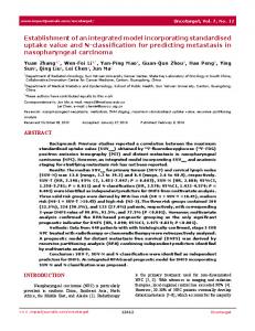
choice dimensions – an MNL model of residential location, ordered logit models of vehicle ownership and bicycle ownership, and an MNL model of commute tour mode choice – and the models are econometrically joined together by the use of common stochastic terms (or random coefficients, or error components) to form a joint model system. The approach circumvents several of the afore-mentioned challenges (such as the explosion of choice alternatives, parameter restrictions, and the restriction to nominal discrete variables) associated with the MNL and/or NL approaches. More importantly, the approach can be used to disentangle a multitude of interdependencies among the choice dimensions of interest, as discussed below. Figure 1 represents various interdependencies among the four choices considered in the paper, including: (1) Causal effects of longer-term choices on shorter-term choices, represented by solid arrows, (2) Residential self-selection effects (represented by the dashed arrows toward the residential location choice box) manifested due to the self-selection of individuals into neighborhoods based on their lifestyle preferences related to auto ownership, bicycle ownership (or bicycling), and commute travel, (3) Endogeneity of auto ownership and bicycle ownership with respect to commute mode choice (represented by the dashed arrows toward auto and bicycle ownership boxes), due to the possibility that individuals’ car ownership and bicycle ownership levels may depend on their commute travel preferences by those modes, and (4) Associative (as opposed to causal) correlations between auto ownership and bicycle ownership due to common unobserved factors influencing both the choices (i.e., common unobserved heterogeneity, represented by the dashed arrow between auto and bicycle ownership boxes). Ignoring any of the latter three effects (i.e., self-selection, endogeneity, or associative correlations) can result in biased estimation of the causal effects and lead to distorted policy implications regarding the influence of various land-use and transportation attributes on longer-term location choices and shorter-term transportation choices. In this paper, an integrated model of residential location, vehicle ownership, bicycle ownership, and commute tour mode choices is estimated using data from the San Francisco Bay Area. There are at least two notable limitations of the current work. First, we consider work location as exogenous, and thus, residential location choice is conditional upon work place. However, for several households, work location may be endogenous to the other choices considered here, especially the residential location choice (Waddell, 1993). The implication of this assumption is that the analyst will not be able to assess the impact of public policies related

5

to housing markets (residential location choice) on labor markets (work location). Another implication is a potential bias in the estimated influence of commute level of service variables on residential location choices, especially when individuals choose their work locations based on their residential locations. Extending the analysis framework to consider the endogeneity of work location is a fruitful avenue for further research. Second, use of cross-sectional data limits us from addressing the issue of temporal dynamics between long-term and short-term choices. As a result, to the extent that some of the households may have made their auto/bike ownership and mode choice decisions prior to their settlement in the current location, one may not be able to clearly decipher the impact of the residential built environment on these decisions. Understanding the dynamics of the interrelationships between the various choice components is an important avenue for future research.

3. ECONOMETRIC MODELING METHODOLOGY 3.1 Model Structure Let the indices q (q = 1, 2, …, Q) , i (i = 1, 2, …, I), and k (k = 1, 2, …, K) represent the decisionmaker, the spatial unit of residence, and the modal alternative, respectively, and the terms n (n = 0, 1, 2,…, N), and m (m = 0, 1, 2, …, M) represent the auto ownership level (i.e., the number of cars) and the bicycle ownership level (i.e., the number of bicycles), respectively. Using these notational preliminaries, the following discussion presents the structure of the model components for each of the four choices (residential location, auto and bicycle ownership and commute tour mode choice), and then highlight the interdependencies among the four components. 3.1.1. The Residential Location Choice Component of the Joint Model System The residential location component takes the multinomial discrete choice formulation as below: sqi* = ϕq' zi + ε qi , spatial unit i chosen if sqi* > max

j =1,2,..., J j ≠i

sqj* , where:

(1)

sqi* is the latent utility that the qth individual obtains from locating in spatial unit i,

zi is a vector of activity-travel environment (ATE) attributes corresponding to spatial unit i, and

ϕq is a coefficient vector capturing individual q’s sensitivity to attributes in zi .

6

Each lth element of ϕq , ϕql corresponds to a specific ATE attribute zil from the vector zi . Each of these elements is parameterized as ϕql = ϕl + Γl' xql + vql + ο ql + π ql + ∑ ωqkl , where: k

xql is a vector of observed characteristics of individual q affecting his/her sensitivity to zil , and vql , ο ql , π ql , and ωqkl (k = 1, 2, 3, …, K) are unobserved factors impacting individual q’s sensitivity to the ATE attribute zil .

vql includes only those unobserved factors that influence sensitivity to residential choice,

ο ql includes the unobserved factors that influence both residential choice and auto ownership, π ql includes the unobserved factors that influence both residential choice and bicycle ownership, ωqkl (k = 1, 2, 3, …, K) terms include only those individual-specific unobserved factors that influence both residential choice and the choice of modal alternative k. Finally, in Equation (1), ε qi is an idiosyncratic error term assumed to be identically and independently extreme-value distributed across individuals and spatial alternatives.

3.1.2. The Auto Ownership and Bicycle Ownership Components of the Joint Model System The Equations (2) and (3), presented below, correspond to the ordered-response structure for auto (or car) ownership and bicycle ownership decisions, respectively. cqi* = α ' xq + δ q' zi + ξ qi , cqi = n if ψ n < cqi* < ψ n +1 ; ψ 0 = −∞,ψ N +1 = +∞ , and

(2)

bqi* = β ' xq + θ q' zi + ζ qi , bqi = m if τ m < bqi* < τ m +1 ;τ 0 = −∞,τ M +1 = +∞ , where:

(3)

cqi* and bqi* represent the latent car ownership and bicycle ownership propensities, respectively,

of the qth individual should his/her household choose to locate in spatial unit i,

xq is a set of sociodemographic characteristics of individual q, zi is the vector of activity-travel environment (ATE) attributes corresponding to spatial unit i.

α , β are coefficient vectors representing the impact of socio-demographics on car ownership and bicycle ownership propensities, respectively.

δ q , θ q are individual-specific coefficient vectors capturing the impact of ATE attributes on car ownership and bicycle ownership decisions, respectively.

δ q and θ q are parameterized as: δ ql = δ l + Λ l' xql + μql ; θ ql = θl + Δ l' xql + ηql , where:

7

xql is a vector of observed characteristics of individual q influencing his/her sensitivity to zil ,

Λ l , Δl are corresponding coefficient vectors in car ownership and bicycle ownership equations,

μql ,η ql capture the impact of unobserved factors that influence the sensitivities to ATE attributes on car ownership and bicycle ownership propensities, respectively. Finally, ξ qi and ζ qi are error terms in the car ownership and bicycle ownership propensity equations, respectively, each of which is partitioned into four components as follows:

ξ qi = ∑ (±ο ql ) zil + ∑ ϑqk + ιq + ∂ qi , and ζ qi = ∑ (±π ql ) zil + ∑υqk ± ιq + ρ qi , where: l

k

l

k

±ο ql terms are common error components related to the sensitivity of the ATE attribute zil in residential location choice and car ownership,

±π ql terms are common error components related to the sensitivity of the ATE attribute zil in residential location choice and bicycle ownership,

∑ϑ

qk

terms include the common error components that capture common unobserved factors

k

affecting car ownership and the utility of mode k,

∑υ

qk

terms include the common error components that capture common unobserved factors

k

affecting bicycle ownership and the utility of mode k,

ιq terms are the common error components capturing the unobserved factors that affect car ownership propensity as well as bicycle ownership propensity,

∂ qi , ρ qi are idiosyncratic terms assumed to be identically and independently standard logistic distributed across individuals and spatial units, in the car ownership and bicycle ownership propensity equations, respectively. The car ownership propensity c qi* and the bicycle ownership propensity bqi* are mapped to the observed car ownership level c qi and the observed bicycle ownership level bqi , using the

ψ and τ thresholds, respectively, in the usual ordered-response fashion.

3.1.3. The Commute Tour Mode Choice Component of the Joint Model System The Equation (4), presented below, corresponds to the MNL structure for mode choice decisions.

8

* * uqkicb = φk' xq + h k cqi + D k bqi + χ qk' zi + ς qkicb , mode k chosen if uqkicb > max

d =1,2,..., K d ≠k

* uqdicb , where:

(4)

* uqkicb is the utility that the qth individual obtains from choosing kth mode for commute should

his/her household choose to locate in spatial unit i and own

cqi

number of cars and bqi

number of bicycles.

xq is a set of socio-demographic characteristics (of individual q) that influences mode choice,

φk is the corresponding coefficient vector in the utility of mode k. h k , D k capture the impact of auto ownership

cqi

and bicycle ownership bqi , respectively, on the

utility of mode k.

zi is the vector of ATE attributes corresponding to spatial unit i,

χ qk is a coefficient vector capturing the impact of ATE attributes zi on the utility for mode k. Each lth element of χ qk , χ qkl corresponds to a specific ATE attribute zil from the vector

zi . Each of these elements is parameterized as follows: χ qkl = χ kl + ϒ 'kl xql + γ qkl , where: xql is a vector of observed factors influencing sensitivity to zil , the lth ATE attribute of zi , ϒ kl

is the corresponding vector of coefficients in the utility of mode k,

γ qkl captures the impact of unobserved terms associated with different sensitivities to ATE attributes in the utility of mode k. Finally, in the Equation (4),

ς qkicb is an error term which is partitioned into four

components as follows: ς qkicb = ∑ (±ωqkl ) zil ± ϑqk ± υqk +℘qkicb , where: l

±ωqkl terms are the common error components related to the sensitivity to ATE attribute zil in residential location choice and mode choice for mode k,

±ϑqk term is the common error component capturing the unobserved factors that affect car ownership propensity and the utility of mode k,

±υqk term is the common error component capturing the unobserved factors that affect bicycle ownership propensity and the utility of mode k, and

9

℘qkicb is an idiosyncratic error term assumed to be identically and independently extreme-value distributed across individuals, modal alternatives, and spatial units.

3.1.4. Interdependencies among the Components of the Joint Model System The Equations (1), (2), (3) and (4) explained in the above three sections may be rewritten as the following joint equation system, with each equation representing one of the four model components – residential location, auto ownership, bicycle ownership, and commute mode choice (the terms in the equations are arranged, with blank spaces, in such a way to show similar elements among different equations in the same column):

sqi* =

∑ (ϕ +Γ x + v )z + ∑ο z + ∑(δ + Λ x + μ z + ∑(±ο + ∑(θ +Δ x +η )z ' l ql

l

ql

il

l

cqi* = α ' xq

l

' l ql

ql ) il

l

bqi* = β ' xq

l

' l ql

ql

u

il

=φ x +hkcqi +Dkbqi +∑(χkl +ϒ x +γqkl )zil ' k q

l

k

l

z)

ql il

l

l

* qkicb

+ ∑π ql zil + ∑∑ωqkl zil

ql il

l

' kl ql

l

+ ∑ϑqk k

+ ∑(±πql zil ) l

+ εqi

+∑±ωqkl zil

+ιq +∂qi

+ ∑υqk ±ιq + ρqi k

±ϑqk ±υqk

+℘qkicb

l

(5) The equation system captures the joint nature of, and the interdependencies among the different model components of, the multidimensional model system employing common stochastic terms,

ο ql zil , π ql zil , ωqkl zil , ϑqk , υqk , and ιq , between the different components of the model system. Each of these common unobserved terms represents a particular type of interdependency between two specific components of the model system, as discussed below. 3.1.4.1. Residential self-selection: The ο ql zil , π ql zil , and ωqkl zil terms capture the jointness of the residential location choice component with the auto ownership, bicycle ownership, and commute mode choice components, respectively. These terms allow self-selection of individuals into neighborhoods based on their unobserved (to the analyst) preferences of auto ownership, bicycle ownership, and commute mode choice, respectively. Such residential self-selection effects are represented by the dashed arrows to the residential location box in Figure 1. To understand this better, consider unobserved factors such as auto disinclination, fitness consciousness and environmental friendliness that make some individuals associate higher utility to bicycle/walk modes, and locate in neighborhoods that allow them to bicycle or walk to work and/or own more bicycles and/or own less cars. In such case, the ωqkl zil terms in the first and fourth equations of

10

Equation system (5) capture the unobserved factors that affect both residential location choice and mode choice preferences, where zil can, for example, be the commute time, and the index k can correspond to bicycle and walk modes. That is, the unobserved factors that affect the sensitivity of commute time in the bicycle/walk modal utilities also affect the sensitivity of commute time in residential location preferences, due to which individuals self select into neighborhoods that are closer to work locations. These common unobserved factors give rise to correlations between residential and modal utilities. The ± sign in front of the ωqkl zil terms in the modal utility equations indicates that the correlation may be positive or negative (one can test the most appropriate signs of correlations). Similarly, the ο ql zil ( π ql zil ) terms capture the unobserved factors due to which individuals may have, for example, lower auto ownership propensity (higher bicycle ownership propensity) and live closer to work locations. Finally, it is important to note here that the model system allows for residential self-selection due to observed individual attributes also (more in Section 5.2). 3.1.4.2. Endogeneity of auto ownership and bicycle ownership in mode choice: The ϑqk and υqk terms capture the jointness of (or the endogeneity of) the auto ownership and bicycle ownership components, respectively, with the mode choice component. Consider, for example, unobserved factors such as social status (physical fitness orientation). Individuals with high social status (physical fitness orientation) may prefer to associate higher car (bicycle) ownership propensity as well as use auto (bicycle) mode for commuting to work. The ϑqk ( υqk ) term captures such unobserved factors and gives rise to correlations between the utility of auto (bicycle) mode and the auto (bicycle) ownership propensity. The correlation in such cases can be expected to be positive, though one can again test the directionality of correlation by experimenting with both the ± signs in the mode utility equation. Such endogeneity effects discussed here are represented by the dashed arrows to the auto ownership and bicycle ownership boxes in Figure 1. Ignoring these endogeneity effects can lead to an inflated influence of auto ownership on auto mode choice and of bicycle ownership on bicycle mode choice. 3.1.4.3. Jointness of auto ownership and bicycle ownership propensities: The ιq term isolates the unobserved factors that affect both auto ownership and bicycle ownership, from those that affect residential location choice or mode choice. These factors include, for example, recreational

11

activity preferences due to which households may own larger number of vehicles (such as SUVs and vans) and use them to carry their bicycles for recreational activities. Ignoring such factors may lead to inflated estimates of the other common unobserved terms and misinform about residential self-selection and endogeneity of auto ownership and bicycle ownership. The arrow between the auto ownership and bicycle ownership boxes in Figure 1 represents this jointness. 3.1.4.4. Causal Relationships: The above three sections discussed the interdependencies among the various choice processes (i.e., the residential location choice, auto ownership, bicycle ownership, and mode choice decisions) due to unobserved factors. These interdependencies can also be termed as associative correlations that do not imply a causal relationship. The primary interdependencies of interest, however, are the causal relationships (represented by the solid arrows in Figure 1) between various choice processes. These relationships are captured by the coefficients of ATE attributes (i.e., the coefficients on the zil terms) in all the equations above, and by the coefficients of auto ownership and bicycle ownership variables (i.e., the coefficients on the

cqi

and bqi terms) in the mode choice equations. The purpose of including the above

discussed common unobserved factors in the model system is to disentangle the “true” impact of the zil ,

cqi

and bqi terms from the associative correlations, in order to be able to carry out

accurate predictions under various policy scenarios.

3.1.5 Discussion The reader will note that our model formulation has parallels with the seemingly unrelated regression (SURE) approach typically used to connect different linear regression equations. In such linear systems, simultaneity between two variables (where one variable appears on the right side of the linear regression formulation of the other variable) implies that the included “endogenous” variable in each equation is correlated with the disturbance term in that equation. Equivalently, in reduced form, the error terms of the two equations get correlated in a specific manner depending upon the structural form of the simultaneity. The only difference is that restrictions imposed on the reduced form by the structural simultaneous equations system must be considered in the simultaneous system, while the seemingly unrelated regressions model imposes no restrictions. Between these two extremes, one can also consider other systems of regression equations (such as random coefficients-based systems) that do not start from a

12

structural system but still impose some structure (relative to the SURE system) in the reduced form system. Thus, even in a linear system, the difference between a simultaneous “integrated” system and a SURE model (or other intermediate structures) for variables is purely based on whether a specific structural model is specified for the endogenous variables or whether the analyst believes that the variables of interest are determined simultaneously but does not know (or would rather not completely specify) a direct structural relationship between the variables. In a discrete choice variable system, things get even more trickier in terms of a clear distinction between a simultaneous system and a SURE type model (In fact, in discrete choice dependent variable systems, a truly simultaneous system, where one variable affects the other and vice versa, is not possible because of identification issues). Specifically, it is typical for discrete choice systems to consider a latent underlying continuous variable system as the generating mechanism to accommodate the discrete nature of the dependent variables. Then, for the latent underlying continuous variable system, one can consider a simultaneous system or a SURE system or other intermediate systems typically considered within the usual linear regression structure (as discussed earlier in this note). But regardless of which system is used for the underlying latent variables, the result is that the discrete variables themselves do get related and become “co-determined”. In this context, the result is an “integrated” discrete variable model system. Intuitively, one way to view this is to consider that the discrete variables are chosen as a package, because of which one discrete variable cannot “cause” the other (but the precursor latent variables can be related to one another). In our integrated system, we model the discrete variables by specifying random coefficients and error components on the underlying latent variable system using an intermediate system formulation. Thus, the sensitivity to observed activity-travel environment attributes in the residential choice utility equations (due to unobserved individual/household tastes) are related to the unobserved auto/bicycle ownership and modal preferences of individuals/households. Such a specification is assumed to be the basis for potential self-selection of individuals/households into specific residential neighborhoods. Similarly, it is assumed that there are common unobserved factors impacting long term mobility decisions (auto ownership and bicycle ownership) and mode choice decisions. 3.2 Model Estimation

The parameters to be estimated in Equation system (5) include: (a) The vectors α , β , φk , ϕ l , δ l , θl , χ kl , Γl , Λ l , Δl , ϒ kl , ψ n ( n = 1, 2, ... N ) and τ m ( m = 1, 2, ...M ) , 13

(b) The scalars h k and D k , and (c) The variances of stochastic components ν ql , μql ,η ql , ο ql , π ql , ωql , ϑqk , υqk ,and ιq (all assumed to be normally distributed with variances σν2ql , σ μ2ql , σ η2ql , σ ο2ql , σ π2ql , σ ω2ql , σ ϑ2qk , σ υ2qk , and σ ι2q ) Let Ω represent a vector that includes all of the parameters to be estimated, let Ω −σ represent a vector of all parameters except the variance terms, let g q be a vector that stacks the ν ql , μql , η ql , ο ql , π ql , ωql , ϑqk , υqk , and ιq terms, let Σ be a corresponding vector of standard errors, let rqj = 1 if individual q resides in spatial unit j and 0 otherwise,

let aqn = 1 if individual q owns n cars and 0 otherwise ( aqn = 1[cqi = n] ), let eqm = 1 if individual q owns m bicycles and 0 otherwise ( eqm = 1[bqi = m] ), and let pqk = 1 if individual q commutes by mode k and 0 otherwise. Then the conditional likelihood function for a given value of Ω −σ and g q for an individual q is: Lq (Ω −σ ) | g q = J

N

M

K

j =1

n =0

m =0

k =1

∏∏∏∏

⎧⎡ ⎡ ⎛ ⎞ ⎤ ⎤ ' ⎪ ⎢ exp ⎢ ∑ ⎜ ϕl + Γ l xql + vql + ο ql + π ql + ∑ ωqkl ⎟ zqil ⎥ ⎥ ⎪⎢ k ⎠ ⎦ ⎥ ⎣ l ⎝ × ⎨⎢ ⎡ ⎛ ⎞ ⎤⎥ ' ⎪⎢ exp x v z ϕ ο π ω + Γ + + + + ∑k qkl ⎟⎠ qjl ⎥ ⎥⎥ ⎢∑ ⎜ l l ql ql ql ql ⎪ ∑ ⎣ l ⎝ ⎦⎦ ⎩ ⎣⎢ j ⎡ ⎛ ⎞ ⎛ ⎞⎤ ' ' ' ' ⎢G ⎜ψ n +1 − α xq − ∑ (δ l + Λ l xql + μql ± ο ql )zil − ∑ ϑqk − ιq ⎟ − G ⎜ψ n − α xq − ∑ (δ l + Λ l xql + μql ± ο ql )zil − ∑ ϑqk − ιq ⎟ ⎥ × l k l k ⎠ ⎝ ⎠⎦ ⎝ ⎣ ⎡ ⎛ ⎞ ⎛ ⎞⎤ ' ' ' ' ⎢G ⎜τ m +1 − β xq − ∑ (θl + Δl xql + η ql ± π ql )zil − ∑υqk − ιq ⎟ − G ⎜τ m − β xq − ∑ (θl + Δ l xql + ηql ± π ql )zil − ∑υqk − ιq ⎟ ⎥ × l k l k ⎠ ⎝ ⎠⎦ ⎣ ⎝ ⎡ ⎡ ' ⎤ ⎤⎫ ⎛ ⎞ ' ⎢ exp ⎢φk xq + h k cqi + D k bqi + ∑ ⎜ χ kl + ϒ kl xql + γ qkl + ∑ ±ωqkl ⎟ zqil ± ϑqk ± υqk ⎥ ⎥ ⎪ l k ⎝ ⎠ ⎣ ⎦ ⎥⎪ ⎢ ⎬ ⎢ ⎡ ' ⎤⎥ ⎛ ⎞ ⎢ ∑ exp ⎢φk xq + h k cqi + D k bqi + ∑ ⎜ χ kl + ϒ 'kl xql + γ qkl + ∑ ±ωqkl ⎟ zqil ± ϑqk ± υqk ⎥ ⎥ ⎪ l k ⎝ ⎠ ⎣ ⎦ ⎦⎥ ⎪⎭ ⎣⎢ k

rqj ×aqn ×eqm × pqk

,

(6) Using the above conditional likelihood function, the unconditional likelihood for the entire data can be computed as: L(Ω) = ∑ ∫ ( Lq (Ω −σ ) | g q ) dF ( g q | Σ) , where F is the multidimensional q gq

cumulative normal distribution. Simulation techniques are applied to approximate the multidimensional integral in the likelihood function, and the resulting simulated log-likelihood function is maximized.

14

4. THE DATA

The primary source of data used for this analysis is the 2000 San Francisco Bay Area Travel Survey (BATS) designed and administered by MORPACE International Inc. for the Bay Area Metropolitan Transportation Commission (MTC). This activity-travel survey collected detailed socio-demographic and comprehensive two-day activity-travel information for individuals from a sample of about 15000 households in the Bay Area. In addition to the 2000 BATS data, several other secondary data sources were used in this analysis. These include: (1) Landuse/demographic coverage data, and zone-to-zone motorized travel level of service files for the bay area, obtained from MTC, (2) GIS layers of bicycling facilities and bicycle network, also obtained from MTC, (3) GIS layers of schools, parks, gardens, restaurants, recreational and other businesses obtained from the InfoUSA business directory, (4) GIS layers of highway and local roadway networks, extracted from the Census 2000 Tiger files, and (5) The Census 2000 population and Housing data summary files (SF1). Using the raw database of the 2000 BATS and the above-identified secondary data sources, several steps were undertaken (details are available with the authors) to create a comprehensive residential location – auto ownership – bicycle ownership – commute tour mode choice database ready for the integrated analysis. This database contained an exhaustive set of socio-demographic and ATE attributes to be explored in the model specification , including: (1) Zonal size and density measures, (2) Zonal land-use structure variables, (3) Regional accessibility measures, (4) Zonal demographics, (5) Zonal ethnic composition measures, and (6) Zonal activity opportunity variables. Such zonal-level built environment measures were created not only for the potential residential location alternatives for each household, but also for the employment locations of all employed individuals residing in the household. The zonal-level characteristics of the employment locations were averaged over all the employed individuals in the household to obtain household level aggregate measures of the activity-travel environment (ATE) in the work locations. In addition to the zonal-level ATE variables, the following variables were extracted and appended to the database: (1) several transportation network level of service (LOS) characteristics by each mode, in and around the residential locations and work locations (such as highway density, bikeway density, and street block density, number of zones accessible by transit from the residential and work locations, number of zones accessible by bike

15

and walk within 6 miles, etc.); (2) individual and household level commute variables (such as travel times and travel costs by each mode, total auto commute travel time for all employed members in the household, travel distance by bike and walk modes, number of commuters in the household that have transit available between home and work zones, number of commuters in the household that have bike route available between home and work zones, etc.). The authors are not aware of any other study in the literature that considers the impact of such a comprehensive set of ATE attributes of both residential and work locations, and commute level of service characteristics. The final estimation sample consists of 5147 adult commuters from 5147 households (one randomly chosen commuter from each household)6 residing in five counties (San Francisco, San Mateo, Santa Clara, Alameda, and Contra Costa) of southern San Francisco Bay area. A descriptive analysis of the estimation data sample indicated the following characteristics of the dependent variables (residential location, auto and bicycle ownership, and commute tour mode choice) in this study. The residential locations belonged to one of the 127 traffic analysis zones (TAZs) of the San Francisco (SF) County, 115 TAZs of the San Mateo (SM) County, 269 TAZs of the Santa Clara (SC) County, 236 TAZs of the Alameda (AL) County, or 154 TAZs of the Contra Costa (CC) County. Out of the 5147 households, 12.3% belonged to SF, 13.6% belonged to SM, 32.7% belonged to SC, 25.7% belonged to AL, and 15.6% belonged to CC Counties. The auto ownership descriptives indicate an average ownership of 1.85 autos per household; 3.5% of the households did not own any automobiles, 33.9% owned one car, 43.1% owned two cars, and 19.4% owned three or more cars. The bicycle ownership descriptives indicate an average bicycle ownership of 1.42 bicycles per household; 36.8% of the households did not own a bicycle, 22.5% owned one bicycle, 20.9% owned two bicycles, and 19.8% owned three or more bicycles. Descriptive analysis of the commute tour mode choice variable indicate the following mode shares: 83.83% auto, 11.47% transit, 1.22% bicycle, and 3.48% walk. The mode shares matched well with the Census journey to work mode shares for each of the 5 counties. Among all 6

Admittedly, modeling the mode choice of only a single commuter per household does not consider all interdependencies between mode choice and other decisions (in Figure 1) in multi-commuter households. For example, in a two commuter household, it is possible that one commuter’s work location and mode choice preferences influence the households’ residential location choice, while the other commuter may simply make the work location and mode choices conditional upon the residential location. Alternatively, both the commuters may have a certain degree of influence on the residential location. Such interdependencies between the mode choice preferences of different commuters and other household level choices in multi-commuter households cannot be captured in the current modeling framework.

16

commute tours, 12.7% involved at least one stop between the origin (home) and destination (work). In a trip-based mode choice analysis, such complex tours would be ignored and the mode shares used for analysis would be skewed.

5. MODEL ESTIMATION RESULTS

Estimation results are presented in Tables 1 through 4, one table for each choice dimension modeled in this paper. This section discusses salient results from these tables. 5.1 Residential Location Choice Model Component Results

Table 1 presents the estimation results for the residential location choice model component. With respect to the residence-end measures, it is found that, after including the zonal transportation network measures and zonal activity opportunity variables in the model, household density and employment density had no significant impact on residential location choice except for certain demographic segments (such as households with seniors and children in the context of household density, and higher income households and Caucasian households in the context of employment density). Thus, it is important to consider the influence of transportation supply and activity opportunities of neighborhoods to avoid over-assessment of the influence of density measures on residential location preferences. The coefficients on the residence-end zonal land-use structure variables suggest that zones with commercial or mixed land uses are less likely to be chosen for residential location. This result may either reflect a preference of households for exclusive residential neighborhoods, or an artifact of the way zones are defined based on land-use homogeneity (i.e., zones with exclusive residential land-uses are categorized as separate zones). Among the residence-end zonal demographics, after controlling for the influence of the housing value variable, the effects of “absolute difference between zonal median income and household income” and “absolute difference between zonal average household size and household size”, indicate that people of similar income levels and race tend to cluster together when it comes to residential location. Similarly, the residence-end zonal race composition measures, when interacted with individual race (see the fourth block of variables in Table 1), also indicate racial clustering. People of a certain race tend to locate in neighborhoods that have a higher fraction of their particular race. Such clustering trends have long been documented in the residential analysis literature (see Waddell, 1993b; Waddell, 2006). 17

The “Residence-end zonal activity opportunity variables” reveal that the availability of destination opportunities such as physically active recreation centers and natural recreation centers makes a neighborhood an attractive residential location. The “Residence-end zonal transportation network measures” show that street block density is negatively associated with residential location choice, particularly for higher income groups, reflecting the preference of high income households for low-density suburban regions with lower density of local streets. The positive coefficient on bicycle facility density (which can be viewed as a surrogate for the bicycle and walk friendliness of the location) suggests that households prefer to live in locations with good infrastructure for bicycling and/walking. Among the household level commute variables, as expected, commute time is negatively associated with residential location choice suggesting that individuals generally try to locate within close proximity of their workplace. However, this tendency appears to be less pronounced for higher income households and more pronounced for lower income households, perhaps because of the ability of the higher income households to afford higher transportation costs. In addition to such income-based heterogeneity, the significant standard deviation of the random coefficient indicates a significant magnitude of unobserved factors influencing households’ sensitivity of residential location choice to commute time. Furthermore, the standard deviation of the random coefficient (i.e., the σ π ql term corresponding to π ql zil in Equation (5)) capturing common unobserved factors π ql in residential location choice and bicycle ownership is found to be significant at the 0.09 level with a negative correlation. As discussed in Section 3.1.4.1, this suggests the presence of significant unobserved factors such as environmental friendliness, bicycling-oriented and/or physically active lifestyles that make people own more bicycles as well as live in (or self-select to live in) residential locations close to the work place (perhaps to enable bicycling to work while staying within a reasonable commute time). These lifestyle preferences constitute unobserved variables or factors influencing both bicycle ownership and residential location. It was found that the neglect of these random coefficients, including the self-selection effects, in the model resulted in an inflated estimation of the negative influence of the commute time variable on residential location and bicycle ownership choices. Finally, transit and bicycle modal accessibility (to work) for commuters in the household positively impacts residential location choice.

18

5.2 Auto Ownership Model Component Results

Table 2 presents the model estimates of the auto ownership component of the model. The coefficients on the residence-end zonal size and density measures indicate that residing in a zone with higher housing or employment density is associated with lower levels of auto ownership, especially so in the case of lower income households residing in high employment locations. However, the standard deviation on the corresponding random coefficient indicates a significant heterogeneity in the influence of household density on auto ownership. Zonal demographic variable effects indicate that households residing in zones with higher fraction of single family dwelling units are likely to own more cars. With respect to commute-related variables, as expected, as the household-level commute time increases, auto ownership increases. However, for lower income households, for whom the transportation costs typically constitute a significant portion of their income, higher auto commute costs are associated with lower auto ownership. Low income households may typically own cars for commuting purposes, among other reasons that necessitate the use of cars. Thus, when the commuting costs are higher, these households may tend to use alternative means of transport and stay in a low-car ownership segment to reduce their transportation costs. Further, higher modal accessibility provided by transit and bicycle is associated with lower levels of auto ownership. Among the residence-end transportation network measures, while neighborhoods with denser highways have higher auto ownership levels, those with higher street block density have lower auto ownership levels. While highway density is indicative of auto-oriented transportation network, street block density is indicative of land uses conducive to travel by walk or bicycle. However, the standard deviation on the random coefficient on street block density suggests a significant variation in the influence of street block density on auto ownership. Higher levels of accessibility by alternative (to auto) modes contribute to lower levels of auto ownership, although again, there appears to be considerable heterogeneity in the influence of transit accessibility. It was found that after including the modal accessibility attributes, the explanatory power of zonal density variables decreased, suggesting that the zonal-density variables often act as proxies for access by modes in explaining auto ownership levels (Bhat and Guo, 2007). The ATE attributes of employment zones such as average bicycling facility density and average street block density negatively impact auto ownership. Presumably these variables signify a greater ability to walk and bike, thus leading to lower car ownership levels for

19

households whose individuals work in such locations. Another important finding in the context of the ATE attributes of employment zones is that the explanatory power of transportation network related variables of the residential locations decreased after including the transportation network related variables of work locations. From a policy perspective, to reduce auto ownership levels, it may not suffice to improve the pedestrian and bicycle facilities in the residential neighborhoods alone; it is important to enhance the walkability and bikeability of different destinations (especially work locations) that people visit. While urban planners may already appreciate the importance of design at both the residential and destination ends of travel, most studies do not include destination attributes in modeling auto ownership and other travel choices. Such studies are likely to be of limited value in assessing the impacts of efforts oriented toward improving the pedestrian, bicycle and transit facilities at work locations, and can potentially overestimate the influence of such policies at the residence-end.. A host of socio-economic and demographic variables appear significant in the model. In the absence of such variables in the model, the magnitudes of the coefficients (and the tstatistics) associated with ATE attributes were considerably higher – thus indicating that the impacts of ATE attributes may be overstated when residential self-selection effects due to observed factors are omitted. For example, higher income households are associated with higher auto ownership levels. At the same time, as discussed in the previous section, higher income households are found to self-select themselves into low density locations. Thus, ignoring the influence of income on auto ownership would result in an over assessment of the density variables on auto ownership levels. The results clearly show the importance of incorporating the influence of socio-demographic factors and unobserved factors (note the significant standard deviations on random coefficients of selected variables including density variables) on auto ownership. In addition to the above findings, there are two significant error correlations that were found to be significant. They are as follows:

Common unobserved factors ( ϑqk ) affecting auto ownership propensity and auto mode choice (standard deviation = 0.4808, t-stat = 3.24, positive correlation, not shown in tables): As discussed in Section 3.1.4.2, this error correlation captures the unobserved auto mode choice preferences that can potentially impact auto ownership levels. For example, auto-inclined lifestyle preferences affect both auto mode utility and auto ownership levels.

20

Common unobserved factors ( ιq ) affecting auto ownership propensity and bicycle ownership propensity (standard deviation = 0.5821, t-stat = 8.60, positive correlation, not shown in tables): The unobserved factors captured by this error component (discussed in Section 3.1.4.3) may include recreational activity preferences due to which households may own a larger number of vehicles and use them to haul their bicycles for recreational activities. The explanatory power of the auto ownership variable in the auto modal utility equation decreased significantly after including the former error component. Ignoring the latter error component resulted in an inflation of the former error component as well as the common error component between residential location choice and bicycle ownership discussed in the previous section. These findings clearly point to the need to disentangle the different unobserved effects that affect multiple choice processes through different error components. Further, since activitytravel environment (ATE) attributes influence mode choice directly as well as indirectly (through their influence on auto and bicycle ownership), it is important to account for the endogeneity of auto ownership and bicycle ownership to appropriately assess the indirect effects of ATE attributes on mode choice. 5.3 Bicycle Ownership Model Component Results

The bicycle ownership model results are presented in Table 3. Bicycle ownership is found to increase with average household income of the residence-end zone. The commute-related variables show that, as commute time of commuters in the household increases, bicycle ownership decreases. However, two findings are noteworthy in the context of bicycle ownership sensitivity to commute time. First, there is significant heterogeneity in the population with respect to sensitivity to this variable as evidenced by the significant standard deviation on its random coefficient. Second, as already discussed in the context of the results presented in Table 1, significant magnitude of common unobserved factors ( π ql ) affect the sensitivity of both residential location and bicycle ownership choices to commute travel time.

Ignoring such

common unobserved factors (or unobserved self-selection effects) resulted in an over-assessment of the influence of commute time on bicycle ownership levels. Bicycle facility density and the availability of activity opportunities such as physically active recreation centers and natural recreation centers are positively associated with bicycle ownership. Finally, a host of socio-economic and demographic variables are found to influence

21

bicycle ownership, several of which have significant impact on residential location choices as well (see Section 5.1). Such common observed factors affecting residential location and bicycle ownership choices suggest the presence of residential self-selection effects due to observed factors, ignoring which would lead to an over assessment of the influence of the ATE attributes. Similar to the common observed and unobserved factors affecting residential location and bicycle ownership choices, a significant magnitude of common unobserved factors were found to influence bicycle ownership and bicycle mode choice to work. This evidenced by the common error component υqk between the bicycle ownership propensity and the bicycle mode choice utility (standard deviation = 0.5165, t-stat = 2.49, positive correlation, not shown in tables), which

accounts for unobserved bicycle mode choice preferences (such as environmental

consciousness) that can potentially impact bicycle ownership levels. Ignoring this error component resulted in an over assessment of the influence of bicycle ownership on bicycle mode choice. 5.4 Mode Choice Model Component Results

Mode choice model estimation results are presented in Table 4. Each variable is denoted with the modal utility equation in which it is included. In general, it is found that several ATE attributes of the residential locations and employment locations (the zonal density measures, land-use structure variables, and transportation system related variables) have a statistically significant influence on mode choice. For example, in the context of residence-end zonal size and density measures and land-use structure attributes, it is found that employment density is positively associated with non-motorized modes, and land-use mix is positively associated with transit mode choice. Further, the standard deviation associated with the random coefficient on the employment density variable is statistically significant suggesting that there are unobserved factors that contribute to significant variation in individual sensitivity to this variable for mode choice to work. Among the residence-end transportation network measures, the positive impacts of street block density on walk mode, bicycle density on walk and bicycle mode, and transit accessibility on transit mode are all intuitive and expected. At the employment location end (see the fourth set of variables), several ATE attributes show a strong influence on commute mode choice – household density and employment density contribute to the choice of transit and walk modes, and bicycle facility density contributes to the choice of bicycle mode. Ignoring these

22

effects resulted in an over assessment of the influence of the corresponding residence-end attributes. Among the level of service variables, as expected, travel time and cost show negative coefficients for all travel modes, and the level of sensitivity to travel cost is greater for individuals from households with lower income. Where the home and work zones are connected by bicycle or walk routes, individuals are more likely to choose the bicycle and walk modes. Activity participation and tour-level variables significantly impact mode choice. For example, combining non-work activities during commutes increases the likelihood of choosing the automobile for travel to work.

Similarly, if an individual undertakes serve passenger,

maintenance, or personal business activities on the travel day, the likelihood of choosing the automobile increases. Interestingly however, participation in discretionary type of non-work activities such as socializing and recreation was not associated with commute mode choice. With respect to the auto ownership and bicycle ownership variables, as discussed earlier in the context of the bicycle and auto ownership model results, the explanatory power of these variables decreased considerably after incorporating the endogeneity of these two variables through common error components ϑqk and υqk . Accounting for such endogeneity allows a more accurate estimation of the impacts of ATE attributes on mode choice, moderated through the influences of such attributes on automobile and bicycle ownership. Finally, several socioeconomic/demographic variables are found to be significant in explaining mode choice (see the eighth set of variables in Table 4); and all of them show expected influences on mode choice. The alternative specific constants shown in the last block of the table do not have a substantive interpretation, but suggest an overall higher preference for the auto mode. One of the key findings in the context of the mode choice model is that zonal density variables became either insignificant or less significant (with lower t-statistics) after adding transportation network variables (various modal accessibility variables). For example, the zonal household density and employment density variables in the utility of the transit mode became insignificant after adding transportation (modal) accessibility variables. Similarly, household density in bike and walk modal utilities, and land use mix in walk utility became insignificant after adding street block density to the modal utility equations. Street block density of work zones in the walk and bike utility equations became insignificant after adding the home-work zone connectivity variables (within 6 miles by bike or within 3 miles by walk). These findings

23

suggest that land use density measures serve as proxies for transportation (modal) availability and accessibility, at least to some extent, in explaining mode choices. Once modal availability/accessibility is accounted for, the land use variables themselves offer modest additional explanatory power. If the modal accessibility variables (i.e., self-selection effects due to observed factors) had been omitted, then the impacts of land use measures on mode choice could have been potentially grossly over-estimated. Another key finding is that the explanatory power of transportation network related variables of the residential locations reduced after including the transportation network related variables of work locations. For example, the variable “number of zones accessible within 30 minutes by transit” became less statistically significant, and the variable “number of zones accessible by transit within 30 to 60 minutes from the residential zone” became insignificant in transit modal utility after adding the transit accessibility variables for the work zones. Similar effects were found with the bicycle facility density variable. Thus, it is important to consider the activity-travel environment attributes of employment locations to avoid over estimation of the impact of residential location attributes in commute mode choice modeling. From a policy standpoint, this result indicates the importance of improving the accessibility of work locations in combination with that of residential locations, to be able to achieve higher non-auto mode shares (Frank et al., 2008, and Maat and Timmermans, 2009 report similar findings regarding the influence of work location attributes on mobility choices). The log-likelihood value at convergence for an independent model system of residential location, auto ownership, bicycle ownership, and mode choice is -37001 (with 108 parameters), while that for the joint model system is -36871 (with 119 parameters). The corresponding loglikelihood ratio statistic is statistically significant at any reasonable level of confidence. This suggests the need to jointly model the multidimensional choice process within an integrated framework even from a model fit stand point.

6. CONCLUSIONS

This paper presents an integrated model system of residential location choice, auto ownership, bicycle ownership, and commute tour mode choice processes. From a substantive viewpoint, this effort embodies the spirit of two major thrusts underlying recent advances in urban travel demand modeling. First, the model system is based on the underlying philosophy that individuals

24

and households make land use and transportation choices as part of a lifestyle package or bundle of decisions that, as evidenced by the findings of this paper, should be modeled simultaneously. Second, consistent with the recent developments in activity- and tour-based modeling, the paper considers mode choice using tours as the unit of analysis. From a methodological standpoint, much of the work in the past has been limited by the complexity associated with estimating simultaneous equation systems that include a multitude of choice dimensions and interdependencies. This paper overcomes these challenges by employing an integrated multi-dimensional choice modeling methodology. The methodology treats residential location as a multinomial logit, auto and bicycle ownership as ordered logits, and commute tour mode choice as a multinomial logit and joins all the model components using common unobserved error components. The methodology explicitly incorporates a series of behavioral aspects (or interdependencies) that are critical to simultaneously modeling multiple choice dimensions. These include: (1) self-selection effects due to observed and unobserved factors (where households locate based on lifestyle and mobility preferences), (2) endogeneity effects (where any one choice dimension is not exogenous to another, but is endogenous to the system), (3) correlated error structures (where common unobserved factors significantly and simultaneously impact multiple choice dimensions), and (4) unobserved heterogeneity (where decision-makers show significant variation in sensitivity to explanatory variables due to unobserved factors). The development and estimation of such a model system constitutes an important step forward in the integrated modeling of land use and transportation choices. Model estimation results using the data from the San Francisco Bay Area highlight the need to model multiple choice dimensions simultaneously to explicitly account for the effects identified above. Model estimation results indicate: (1) significant residential self-selection effects, for example, where individuals with certain modal preferences (either in auto/bicycle ownership or mode choice) are found to self-select into residential zones that support their preferences, (2) significant endogeneity effects, for example, where auto ownership and bicycle ownership are endogenous to mode choice decisions, (3) significant presence of common unobserved factors affecting multiple choice dimensions, for example, in the case of auto ownership and bicycle ownership, and (4) significant unobserved heterogeneity, for example, where households showed significant variance in sensitivity to commute travel time in making residential location choices (due to unobserved factors). More importantly, ignoring any of these

25

effects resulted in biased estimation of the other effects, as well as that of the coefficients of the activity-travel environment attributes in the model system. Thus, from a policy standpoint, to be able to forecast the “true” causal influence of activity-travel environment changes on residential location, auto/bicycle ownership, and commute mode choices, it is necessary to jointly model the multiple choice dimensions in an integrated framework. Unfortunately, most land-use and travel forecasting model systems in place today treat multi-dimensional choice processes as a series of sequential independent decisions or attempt to connect the various decisions through the use of deeply nested logit models that are quite restrictive with regard to their ability to reflect the various aspects of behavior highlighted in this paper. Given recent advances in analytical and computational methods, a fruitful avenue for further research is to investigate ways to implement integrated models of the type developed in this paper in large-scale land-use and travel forecasting model systems. Another useful avenue for further work is to integrate additional model components such as work location choice into the proposed modeling framework.

ACKNOWLEDGEMENTS

The authors appreciate the useful comments of four anonymous reviewers on an earlier manuscript.

REFERENCES

Abraham, J.E., and J.D. Hunt (1997) Specification and Estimation of Nested Logit Model of Home, Workplaces, and Commuter Mode Choices by Multiple-Worker Households. Transportation Research Record 1606, pp. 17-24. Anas, A. (1981) The Estimation of Multinomial Logit Models of Joint Location and Travel Mode Choice from Aggregated Data. Journal of Regional Science 21(2), pp. 223-242. Anas, A. (1995) Capitalization of Urban Travel Improvements into Residential and Commercial Real Estate: Simulations with a Unified Model of Housing, Travel Mode and Shopping Choices. Journal of Regional Science 35(3), pp. 351-375. Anas, A., and L.S. Duann (1985) Dynamic Forecasting of Travel Demand, Residential Location, and Land Development: Policy Simulations with the Chicago Area Transportation/LandUse Analysis System. Papers in Regional Science Association 56, pp. 38-58. Ben-Akiva, M., and I. Salomon (1983) The Use of the Lifestyle Concept in Travel Demand Models. Environment and Planning A 15, pp. 623-638. Ben-Akiva, M, and S.R. Lerman (1985). Discrete choice analysis: Theory and application to travel demand. MIT Press Series in Transportation Studies. Cambridge, Massachusetts; London, England:The MIT Press. Ben-Akiva, M., and J.L. Bowman (1998) Integration of an Activity-based Model System and a Residential Location Model. Urban Studies 35(7), pp. 1131-1153.

26

Bhat, C.R., and J.Y. Guo (2007) A Comprehensive Analysis of Built Environment Characteristics on Household Residential Choice and Auto Ownership Levels. Transportation Research 41B(5), pp. 506-526. Brown, B. (1986) Modal choice, location demand, and income. Journal of Urban Economics 20, pp. 128–139. Cao, X., P.L. Mokhtarian, and S.L. Handy (2006) Examining the Impacts of Residential Selfselection on Travel Behavior: Methodologies and Empirical Findings. Research Report: UCD-ITS-RR-06-18, Institute of Transportation Studies, University of California, Davis. Desalvo, J.S., and M. Huq (2005) Mode choice, commuting cost, and urban household behavior. Journal of Regional Science 45, pp. 493–517. Eliasson, J., and L. Mattsson (2000) A Model for Integrated Analysis of Household Location and Travel Choices, Transport Research 34A, pp. 375-394. Frank, L., M.A. Bradley, S. Kavage, J. Chapman, and Keith Lawton Consulting (2008) Urban Form, Travel Time, and Cost Relationships with Tour Complexity and Mode Choice. Transportation 35, pp. 37-54. Lerman, S.R (1976) Location, Housing, Automobile Ownership and Mode to Work: A Joint Choice Model. Transportation Research Record 610, pp. 6-11. Leroy, S.F., and J. Sonstelie (1983) Paradise lost and regained: transportation innovation, income and residential location. Journal of Urban Economics 13, pp. 67–89. Maat, K., and H.J.P. Timmermans (2009) Influence of the residential and work environment on car use in dual-earner households. Transportation Research Part A 43, pp. 654-664. Miller, E. J., and P.A. Salvini (2001). The integrated land use, transportation environment (ILUTE) microsimulation modelling system: Description and current status. In D. A. Hensher (Ed.), Travel Behaviour Research: The leading edge (pp. 711-724). Amsterdam; New York: Pergamon Press. Pinjari, A.R., R.M. Pendyala, C.R. Bhat, and P.A. Waddel (2007) Modeling Residential Sorting Effects to Understand the Impact of the Built Environment on Commute Mode Choice. Transportation 34, pp. 557-573. Salon, D. (2006) Cars and the City: An Investigation of Transportation and Residential Location Choices in New York City. Dissertation, Department of Agricultural and Resource Economics, University of California, Davis. Salvini, P. A., and E.J. Miller (2005). ILUTE: An operational prototype of a comprehensive microsimulation model of urban systems. Networks and Spatial Economics, 5(2), pp. 217-234. Strauch, D., Moeckel, R., Wegener, M., Gräfe, J., Mühlhans, H., Rindsfüser, G.. (2005). Linking transport and land use planning: The micoscopic dynamic simulation model ILUMASS. In P. M. Atkinson, G. M. Foody, S. E. Darby, & F. Wu (Eds.), Geodynamics (pp. 295-1 311). Boca Raton, 2 Florida: CRC Press. Vega, A., and A. Reynolds-Feighan (2009) A methodological framework for the study of residential location and travel-to-work mode choice under central and suburban employment destination patterns. Transportation Research Part A, 43, pp. 401-409. Waddell, P. (1993a) Exogenous Workplace Choice in Residential Location Models: is the Assumption Valid in a Multinodal Metropolis? Geographical Analysis 25(1), pp. 65-82. Waddell, P. (1993b) A Multinomial Logit Model of Race and Urban Structure. Urban Geography, 13(2), pp. 127-141.

27

Waddell, P. (2001) Towards a Behavioral Integration of Land Use and Transportation Modeling. In D. Hensher, (Ed.), Travel Behavior Research: The Leading Edge, New York: Pergamon, pp. 65-95. Waddell, P. (2002). UrbanSim: Modeling urban development for land use, transportation, and environmental planning. Journal of American Planning Association, 68, pp. 297-314. Waddell, P. (2006) Accessibility and Residential Location: The Interaction of Workplace, Housing Tenure, Residential Mobility and Location Choices. In Modelling Residential Location Choice, John Preston, Francesca Pagliara and David Simmonds eds. Ashgate. Waddell, P., L. Wang, and X. Liu (2008) UrbanSim: An Evolving Planning Support System for Evolving Communities. Planning Support Systems for Cities and Regions, edited by Richard Brail. Cambridge, MA: Lincoln Institute for Land Policy, pp. 103-138. Wegener, M., P. Waddell and I. Salomon. (2001). Sustainable Lifestyles? Microsimulation of Household Formation, Housing Choice and Travel Behaviour. Social Change and Sustainable Transport. W. Black and P. Nijkamp, (eds.) Bloomington, IN: Indiana University Press.

28

Residential Location Choice

Auto Ownership

Bicycle Ownership

Activity-travel Choices (e.g. Commute Mode Choice)

Figure 1. Interdependencies between Residential Location, Auto and Bicycle Ownership, and Commute Mode Choices

29

Table 1. Estimation Results of the Residential Location Choice Component of the Joint Model Variables

Parameter

t-stat

0.838 0.000 -0.479 -0.217 -0.002 -0.077 -0.034 -0.011

29.67 Fixed -5.82 -2.86 -0.80 -1.94 -1.77 -1.65

Fraction of commercial land area Land-use mix Residence-end zonal demographics

-0.683 -0.395

-5.31 -4.47

Median housing value in the zone Absolute difference between zonal median income and household income ($ x 10-3) Absolute difference between zonal average household size and household size Residence-end zonal race composition measures

-0.133 -0.016 -0.345

-10.48 -15.96 -8.90

Fraction of African-American population interacted with African-American dummy variable Fraction of Asian population interacted with Asian dummy variable Fraction of Caucasian population interacted with Caucasian dummy variable Fraction of Hispanic population interacted with Hispanic dummy variable Residence-end zonal activity opportunity variables

3.239

6.83

2.476 1.713 1.666

8.26 13.86 3.72

0.027

5.25

0.046

2.27

-0.031

-5.56

-0.039 0.018

-3.89 2.97

-0.064 -0.034 0.007 0.041 0.006

-23.69 -5.10 2.31 16.29 1.69

0.306

6.96

0.272

7.00

Residence-end zonal size and density measures Logarithm of number of households in zone Household density (#households per acre x 10-1) Interacted with presence of seniors in household Interacted with presence of children (of age 5 to 15 years) in household Employment density (#jobs per acre x 10-1) Interacted with household income greater than $ 90,000 per annum Interacted with household belonging to the Caucasian race Interacted with presence of children (of age 15 years or younger) in household Residence-end zonal land-use structure variables

Number of physically active recreation centers such as fitness centers, sports centers, dance and yoga studios Number of natural recreational centers such as parks, gardens, etc. interacted with Number of bicycles in the household Residence-end zonal transportation network measures Street block density (number of blocks per square mile x 10-1) Interacted with household income greater than $ 90,000 per annum Bicycling facility density (miles of bike lanes per square mile) Household level commute variables Total commute time (by auto) of all commuters in the household (minutes) Interacted with household income less than $ 35,000 per annum Interacted with household income greater than $ 90,000 per annum Standard deviation Standard deviation of the random coefficient capturing common unobserved factors in residential location and bicycle ownership choices (negative Number of commuters in the household with home and work zones connected by transit within 30 minutes Number of commuters in the household with home and work zones connected by bike route of less than 6 miles length

1 Mile = 1.609 Kilometers, 1 Square Mile = 2.59 Square Kilometers, 1 Acre = 0.004046 Square Kilometers

30

Table 2. Estimation Results of the Auto Ownership Component of the Joint Model Variables

Parameter

t-statistic

-0.031 0.056 -0.091 -0.045

-2.44 3.84 -1.80 -3.42

Fraction of single family housing units Commute-related variables

0.382

1.79

Total commute time (by auto) of all commutes in household (minutes) Total commute cost by (auto) of all commutes in household ($) interacted with household income less than $ 35,000 per annum Number of commuters in the household with home and work zones connected by transit within 30 minutes Number of commuters in the household with home and work zones connected by bike route of less than 6 miles length Residence-end local transportation network measures

0.003 -0.260

1.67 -2.58

-0.207

-2.07

-0.099

-1.33

Density of highways (miles per square mile) Street block density (number of block per square mile x 10-1) Standard deviation Number of zones accessible within 30 minutes by transit Standard deviation Number of zones accessible within 6 miles by bicycle ATE Attributes of Employment Zones

0.063 -0.023 -0.008 -0.011 0.025 -0.003

1.38 -1.53 -5.65 -1.97 -3.34 -1.21

Average bicycling facility density (miles of bike lanes per square mile) of the employment locations of all commuters in the household Average street block density (number of street blocks per square mile) of the employment locations of all commuters in the household Standard deviation Household demographic variables

-0.028

-1.88

-0.003

-4.56

0.002

1.24

1.688 1.783 0.120 0.772 -0.877 0.548 -1.168 -1.374 -0.252 0.279 0.143 0.782 0.831 -0.366

14.90 11.45 2.15 8.22 -5.16 5.96 -4.69 -9.40 -1.99 3.68 1.66 7.11 7.90 -1.68

Residence-end zonal size and density measures Household density (#households per acre x 10-1) Standard deviation Employment density (#employment per acre x 10-1) Interacted with household income less than $ 35,000 per annum Residence-end zonal demographics

Number of active adults Number of senior adults Number of children (of age 5 to 15 years) in household Number of employed individuals Number of physically challenged individuals Household income ($ x 10-5) Single parent household Single individual household Age of householder is less than 30 years Householder is male Caucasian household Residing in a single-family housing unit Own household dwelling Residing in San Francisco County

31

Table 3. Estimation Results of the Bicycle Ownership Component of the Joint Model Variables

Parameter

t-statistic

0.438

2.77

-0.023 0.009 0.006

-1.59 2.42 1.69

Bicycling facility density (miles of bike lanes per square mile) Residence-end zonal activity opportunity variables

0.040

3.27

Number of physically active recreation centers such as fitness centers, sports centers, dance and yoga studios Number of natural recreational centers such as parks, gardens, etc. interacted with Number of bicycles in the household Household demographic variables

0.016

1.51

0.053

1.34

0.371 0.491 1.153 0.332 0.464 -0.386 -0.762 0.144 0.666 0.470 0.302

5.58 6.63 13.44 5.04 6.20 -3.56 -6.41 2.35 8.86 5.68 3.76

Residence-end zonal demographics Average household income in the zone Commute-related variables Total commute time (by auto) of all commutes in household (minutes x 10-1) Standard deviation Standard deviation of the random coefficient capturing common unobserved factors in residential location and bicycle ownership choices (negative correlation) Residence-end local transportation network measures

Number of active adults Number of children (of age less than 5 years) in household Number of children (of age 5 to 15 years) in household Number of students in the household Household income ($ x 10-5) Single individual household Age of householder is less than 30 years Householder is male Caucasian household Residing in a single-family housing unit Own household dwelling

32

Table 4. Estimation Results of the Mode Choice Component of the Joint Model Variables

Parameter

t-stat

Residence-end zonal size and density measures (including demographic interactions) Employment density (#jobs per acre x 10-1) – Bicycle and Walk modes Standard deviation Residence-end zonal land-use structure variables

0.017 0.046

1.67 2.39

Land-use mix – Transit mode Residence-end zonal transportation network measures Street block density (number of blocks per square mile x 10-1) – Walk mode

0.621

1.91

0.041 0.042 0.070 0.011

1.71 1.00 1.85 2.67

0.015 0.021 0.017 0.012 0.101 0.032

2.18 1.50 3.83 1.49 2.70 9.07

-0.031 -0.342 -0.508 1.132

-8.39 -9.29 -2.15 3.99

1.616

3.63

Individual undertakes pick-up/drop-off activity – Auto mode Individual undertakes maintenance activity – Auto mode Individual undertakes personal business activity – Auto mode Tour involves at least one non-work stop – Auto mode Household vehicle ownership and bicycle ownership

0.842 0.248 0.553 1.725

4.42 1.62 3.49 4.92

Number of vehicles owned by the household – Auto mode Number of bicycles owned by the household – Bicycle mode Individual and household sociodemographic and economic variables

0.435 0.292

5.27 3.79

-1.417 1.681 0.219

-4.61 4.30 1.65

-0.495 -1.975 -1.266

-1.05 -3.45 -1.90

Bicycling facility density (miles of bike lanes per square mile) – Bicycle mode Bicycling facility density (miles of bike lanes per square mile) – Walk mode Number of zones accessible within 30 minutes by transit – Transit mode ATE attributes of employment zones Household density (#households per acre x 10-1) – Transit mode Household density (#households per acre x 10-1) – Walk mode Employment density (#jobs per acre x 10-1) – Transit mode Employment density (#jobs per acre x 10-1) – Walk mode Bicycle facility density (miles of bike lanes per square mile) – Bicycle mode Number of zones accessible within 30 minutes by transit Level of service variables (including demographic interactions) Travel time between home and work zones – All modes Travel cost between home and work zones – All modes Interacted with household income less than $ 35,000 per annum – All modes Home and work zones connected by a bicycle route of length less than 6 miles – Bicycle mode Home and work zones connected by walk route of length less than 3 miles – Walk Activityd participation and tour-level variables

Individual is a female – Bicycle mode Individual has a drivers license – Auto mode Individual has an inflexible work schedule – Auto mode Alternative specific constants (Auto is the base alternative) Transit Bicycle Walk

33