Dec 30, 2010 - define a tree with 7117 nodes and 1 348 709 edges. Since ... top to bottom; the seed enzymes as root nodes are omitted for simplicity. b.
CHAOS 20, 045115 共2010兲
Modeling the complex dynamics of enzyme-pathway coevolution Moritz Schütte,1,2 Alexander Skupin,1 Daniel Segrè,2,3 and Oliver Ebenhöh1,4 1
Max Planck Institute of Molecular Plant Physiology, Am Mühlenberg 1, 14476 Potsdam-Golm, Germany Bioinformatics Program, Boston University, Boston, Massachusetts 02215, USA 3 Department of Biology and Department of Biomedical Engineering, Boston University, Boston, Massachusetts 02215, USA 4 Institute of Medical Sciences and Institute of Complex Systems and Mathematical Biology, SUPA, University of Aberdeen, Aberdeen AB24 3UE, United Kingdom 2
共Received 24 August 2010; accepted 29 November 2010; published online 30 December 2010兲 Metabolic pathways must have coevolved with the corresponding enzyme gene sequences. However, the evolutionary dynamics ensuing from the interplay between metabolic networks and genomes is still poorly understood. Here, we present a computational model that generates putative evolutionary walks on the metabolic network using a parallel evolution of metabolic reactions and their catalyzing enzymes. Starting from an initial set of compounds and enzymes, we expand the metabolic network iteratively by adding new enzymes with a probability that depends on their sequence-based similarity to already present enzymes. Thus, we obtain simulated time courses of chemical evolution in which we can monitor the appearance of new metabolites, enzyme sequences, or even entire organisms. We observe that new enzymes do not appear gradually but rather in clusters which correspond to enzyme classes. A comparison with Brownian motion dynamics indicates that our system displays biased random walks similar to diffusion on the metabolic network with long-range correlations. This suggests that a quantitative molecular principle may underlie the appearance of punctuated equilibrium dynamics, whereby enzymes occur in bursts rather than by phyletic gradualism. Moreover, the simulated time courses lead to a putative time-order of enzyme and organism appearance. Among the patterns we detect in these evolutionary trends is a significant correlation between the time of appearance and their enzyme repertoire size. Hence, our approach to metabolic evolution may help understand the rise in complexity at the biochemical and genomic levels. © 2010 American Institute of Physics. 关doi:10.1063/1.3530440兴 Evolution is a dynamic process in which species become extinct and new species emerge all the time. It is a disputed question whether the emergence of new species proceeds with an approximately constant rate or whether new species rather evolve in short periods with a high speciation rate which are separated by long silent periods in which only few new species evolve. The latter scenario is referred to as “punctuated equilibrium” and has recently received support from empirical evidence. Here, we present a model of metabolic evolution which suggests that punctuated equilibria can also be observed in the evolution of macromolecules. This finding also supports the hypothesis that underlying molecular mechanisms may be responsible for the phenomenon of punctuated equilibrium in the evolution of new species. Our model uses available amino acid sequences for thousands of enzymes present in several hundred different organisms. By comparing all these sequences, we estimate probabilities that sequences may have evolved from one another. This information allows us to simulate putative scenarios for how today’s metabolism might have evolved. By time series analysis we demonstrate that the existing sequence information strongly suggests a punctuated equilibrium behavior, which is considerably less pronounced if sequence information is deliberately neglected.
1054-1500/2010/20共4兲/045115/10/$30.00
I. INTRODUCTION
The evolution of the modern biochemical pathways from an early protometabolism must have been shaped by innovations concurrently involving enzymes and chemical compounds.1–3 While it is generally assumed that today’s enzymes have evolved from a few ancestors that were able to catalyze the first reactions, the details of this evolutionary history are almost as uncertain as the details about the first self-replicating systems themselves.4–9 Several scenarios have been proposed, the simplest suggesting a “forward” evolution in which enzymes evolved that could make use of the end products of existing metabolic pathways.10 In the reverse assumption of a retrograde evolution, a necessary precursor became depleted and enzymes have evolved that replenish this required resource from other, still abundant, substances.11 While supporting example pathways may be found for both views, the more complex assumption of a patchwork evolution12,13 becomes more relevant when viewing metabolism as a whole. The method of network expansion14,15 provides a simple evolutionary model that extends the forward evolution scenario to the metabolic network comprising all biochemical reactions known to date. While this approach was useful to relate structural to functional properties16 by tracing catalytic properties along the evolutionary tree,17 discovering hints for an early separation of DNA and RNA metabolism18 and providing insight into
20, 045115-1
© 2010 American Institute of Physics
Downloaded 02 Jan 2011 to 128.197.39.31. Redistribution subject to AIP license or copyright; see http://chaos.aip.org/about/rights_and_permissions
045115-2
Schütte et al.
the increase of complexity upon the rise of oxygen in the Earth’s atmosphere,19 it is clearly too simple to reproduce realistic evolutionary paths. More recent models elaborating on these ideas include the toolbox model of metabolic evolution,20 which assumes that network evolution is driven by the need to explore new resources and can readily explain the apparent quadratic scaling of the numbers of transcription factors with the total number of genes. The view of metabolic evolution as a Markov process in which additions or removal of reactions depend on the numbers of neighboring reactions21 allows one to estimate parameters for the evolutionary dynamics and to assess possible evolutionary paths between two different network configurations. The above mentioned examples all provide plausible arguments for a particular evolutionary path, but do not explicitly take into account that after the appearance of the first catalyzed reaction networks, the discovery of new chemical compounds is strongly linked to the evolution of new enzymes from existing ones. Hints that the evolution of the sequence space defining contemporary enzymes mirrors to some extent the gradual expansion of the chemical space, defined by the variety of metabolites, were recently found by correlating sequence similarities to a distance of the catalyzed reactions on the metabolic network.22 It was argued23 that such a coevolution promotes short term avalanches during which a large number of new enzymatic steps could be invented, thus giving rise to a punctuated equilibrium behavior.24,25 In this paper, we present a model of metabolic evolution combining genome scale data, tools from bioinformatics, and dynamic modeling and time series analysis with the goal of studying the apparent coevolution of small molecules and catalysts in further detail. As a basis for our exploration, we use the KEGG database26,27 which provides a comprehensive collection of biochemical reactions from several hundred organisms and information on amino acid sequences of the respective catalyzing enzymes. While previous models28–30 investigated the evolution of metabolic networks as idealized artificial processes, our current model explicitly considers available biological data and assumes that those enzymes are more likely to evolve for which a related enzyme has already been discovered. We systematically explore how the evolutionary dynamics depends on the coevolution of metabolites and enzymes by introducing a tunable parameter reflecting the importance of sequence similarity. Thus, we can separate the effects of a sequence-based evolution from one in which the discovery of new enzymes is only restricted by stoichiometric constraints. We find that simulations taking into account existing sequence data display a punctuated equilibrium behavior and thus support the view that evolution, also at the level of metabolic networks, occurs in bursts of rapid sequences of new inventions, rather than in a gradual fashion.24 II. MODEL DESCRIPTION
The enzymes found in contemporary organisms are highly efficient and usually very specific catalysts for chemical reactions. The amino acid sequences of present-day enzymes are the outcome of a long evolutionary history, in
Chaos 20, 045115 共2010兲
which they were subjected to random mutations and selective pressures favoring only particular sequences which may efficiently perform useful functions. A difficulty in modeling the evolutionary process of enzyme evolution is that neither sequences for early or extinct enzymes nor the precise criteria for the selective pressures are known. Our proposed simple model for the evolution of metabolism takes these limitations into account. Instead of aiming at describing the evolution of networks of particular organisms, we focus on the network comprising reactions from several hundreds of species. We can thus focus on very general selective principles and ignore the specific pressures that were acting to support the evolution of highly specialized functions. Due to the lack of knowledge of early and now extinct protein sequences, our model is limited to all described biochemical reactions and sequence information available to date. We mimic the evolution of the network comprising the presently known metabolic reactions by a simple process in which the network grows in size by consecutive addition of single enzymes. The process is initiated by assuming that a certain combination of primitive metabolites is abundant in the environment. We assume that new enzymes may evolve from existing ones through a series of amino acid exchanges. Since the mechanism for such mutations is essentially a random process, we assume that the probability to discover a new functional enzyme from an existing one is higher, the more similar their corresponding sequences are. Thus, at any stage of our simulated evolutionary process in principle every known enzyme may evolve. However, we assume that only those newly discovered enzymes will be positively selected which can perform a useful function. We therefore impose a selective pressure by accepting only those new enzymes which can catalyze a biochemical reaction from reactants that may in principle be produced from reactions already present in the network. A temporal scale is introduced by assuming that evolutionary events with a higher probability tend to occur faster. The evolutionary simulation is implemented as a Gillespie algorithm31 for the simulation of stochastic expansion processes and can be summarized in the following seven steps: 共1兲 A set of primitive compounds and first enzymes is selected. These comprise the initial network. 共2兲 On the basis of the actual network structure, all enzymes that can catalyze a reaction utilizing only substrates present in the network are identified. For each enzyme i, a propensity pi is calculated based on the sequence similarity to already present enzymes 共see below兲. The propensity describes the probability that the enzyme is discovered per unit time. 共3兲 Depending on the propensities, the time tnext of the next evolutionary event is determined by an exponentially distributed random variable with the mean given by 1 / 兺pi. 共4兲 Which particular enzyme is added at time tnext is determined by a uniformly distributed random number. The probability that enzyme j is selected is given by p j / 兺pi.
Downloaded 02 Jan 2011 to 128.197.39.31. Redistribution subject to AIP license or copyright; see http://chaos.aip.org/about/rights_and_permissions
045115-3
Chaos 20, 045115 共2010兲
Enzyme-pathway coevolution
共5兲 All reactions catalyzed by the selected enzyme as well as the corresponding products are added to the network. 共6兲 Due to the incorporation of new substances, new reactions catalyzed by enzymes already present in the network may be executable. These reactions and their products are added as well. The same holds true for any newly occurring spontaneous reactions. 共7兲 The process is repeated with step 共2兲 until no new enzymes can be added to the network. Iterating this expansion process leads to a series of invented enzymes whose invention times depend on the underlying dynamics. Hence, we use the interenzyme intervals 共IEIs兲, which are defined by the sequence of tnext and correspond to waiting times, to characterize the evolutionary process. In contrast to the conceptually similar method of network expansion introduced in Ref. 15, in our model enzymes are considered to be the basic units of the networks rather than reactions. As a consequence, the discovery of a new enzyme leads to the addition of all reactions that such enzyme can catalyze. Moreover, whereas in the method of network expansion all reactions which can possibly occur are simultaneously added to the growing network in each step, here we only add a single enzyme in each expansion event. Defining probabilities for enzyme appearance introduces a stochastic component which is inherent to all evolutionary processes. Further, by assigning characteristic times for the single evolutionary events our model possesses an intrinsic definition of an evolutionary time coordinate. Like in many applications of the method of network expansion 共see, e.g., Refs. 32 and 33兲, we also assume that common cofactors do not specifically have to be produced during the expansion process before they can be used 共see Sec. IV兲. The rationale for this is that their metabolic functions can in principle also be carried out by simpler pairs of molecules. For example, the transfer of phosphate groups by ATP/ADP is possible by pyrophosphate and phosphate, as demonstrated in the bacterial phosphotransferase system, the role of NADH/ NAD+ as electron carriers can in principle be performed by metal ions such as Fe2+ / Fe3+ with different oxidation states.
III. SEQUENCE DISTANCES AND PROPENSITIES
One particular focus of our model is the investigation of the evolutionary dynamics for different assumptions on how strongly the evolvability of novel enzymes from existing ones depends on the respective sequence similarities. For roughly half of all functionally different enzymes present in the KEGG database,27 sequence information is available. The amount of information for one particular enzyme commission 共EC兲 number can vary between none and a couple of thousand different sequences. In total, KEGG 共release 53兲 provides around 1 ⫻ 106 sequences from various organisms for about 3000 EC numbers. We reduced the space of possible sequences by construction of a consensus set using the clusters of orthologous groups 共COG兲 of proteins database34–37 as a benchmark. This enables to drop redundant sequences between functionally equivalent enzymes having
the same EC number, see Ref. 22 and Sec. IV. Herewith, we obtain a set of 11 925 sequences that code for 3048 EC numbers for which we calculate all mutual distances using the “score” of the best BLAST alignment to assess the probability that sequence A evolves into B. The Blast score provides putative evolutionary knowledge about single amino acid substitutions, insertions, and deletions from which we define the distance between sequence A and sequence B as 2 · score共A,B兲 . score共A,A兲 + score共B,B兲
DAB = 1 −
共1兲
The pairwise distance ranges from 0 for identical sequences to 1 for sequences without any significant alignment. For EC numbers for which no sequence is available, we assign distances to all other enzymes randomly from the distribution of all calculated sequence distances. While it is certainly possible that this introduces a bias in our results, we consider this approach as the best possibility under the circumstances of incomplete information. It is plausible to assume that during evolution, the probability to discover a new enzyme is higher, if a similar enthe minimal distance zyme already exists. We denote by dmin i for enzyme i to all enzymes that have already been found. To have a tunable parameter that weighs the strength of the influence of the protein sequences, we define the propensities for a new enzyme to be discovered by pi =
1 ␥ dmin i
.
共2兲
This definition implies that we assume that the expected time to find a new enzyme depends only on the minimal distance to existing enzymes scaled by the exponent ␥. The extreme assumption of ␥ = 0 leads to equal propensities for all possible new enzymes and thus reflects a hypothetical case in which sequence information has no influence on the selective process, and the evolution of the network is exclusively determined by chemical constraints. A value of ␥ = 2 corresponds to the assumption that the possible sequence space is explored in a process analogous to a random walk, for which the average distance covered is proportional to the square root of the elapsed time. The other extreme ␥ → ⬁ reflects the hypothetical case of the path following least resistance in which the enzyme with the closest distance to an existing enzyme will always be discovered in the next step.23,38 IV. METHODS A. Data for network structure and sequences
We use the KEGG database, release 53. The “genes.pep” in fasta format is downloaded for protein sequences and the ligand-file for reactions. In order to curate the data, erroneous reactions, which are not balanced or contain unspecified parts like a rest group, are rejected. The irreversibility information is obtained by scanning the pathway maps.32,44 Reactions that contain the cofactor pairs ATP/ADP, NAD/NADP, NADH/NADPH, or Co-A/acetyl-CoA are added a second
Downloaded 02 Jan 2011 to 128.197.39.31. Redistribution subject to AIP license or copyright; see http://chaos.aip.org/about/rights_and_permissions
045115-4
Schütte et al.
time without the cofactors, assuming that they are possible during expansion without coupling to cofactor usage and production. B. Sequence distance and consensus set
In order to calculate the evolutionary distance between any two enzymes, we use pairwise sequence alignment using BLAST 共version 2.2.22, standalone blast, http:// www.ncbi.nlm.nih.gov/blast/blast_overview.shtml兲 bl2seq -i SequenceA -j SequenceB -p blastp -F F -o output with the default substitution matrix BLOSUM62. Then we score the alignment by the best hit of the score from the output getting the distance DAB given by Eq. 共1兲. This is not a distance by mathematical definition as it does not fulfill the triangular inequality. It ranges from 0, identical, to 1, completely different.22 KEGG release 53 contains around 1 ⫻ 106 sequences containing an EC number in their description. We sort these sequences by EC numbers and choose representatives from each set by taking only into account those that have a mutual distance, defined similarly to Eq. 共1兲, above 0.95 and drop all others. The cutoff has been chosen according to a benchmark using the COG of proteins database.22,34 This reduces the sequence set to 11 925 for 3048 EC numbers. For EC numbers that appear in the reaction set but for which we do not have a sequence, we randomly pick a distance to any other sequence from the distribution of distances between all known ones. C. Seeds
What are the first metabolites and enzymes? We use the following primordial seed of compounds: H2O, CO2, H2SO4, H3PO4, NH3, and H+.1,45 In order to identify the putative first enzymes, we use the work by Sobolevsky46–48 who identified the common conserved protein fragments in 131 proteomes. One particularly long fragment LSGGQQQRVAIARAL was found in bmn:BMA10247 1739 and tpe:Tpen 0904 and we added the remaining two of the same function 3.6.3.21, eco:b2306 and hpa:HPAG1 0922, to the seed of enzymes. V. RESULTS A. The expansion: Process and enzyme sequences
The expansion process starts from a given set of metabolites and enzymes called the seed.14–17 This set represents a putative prebiotic chemical environment. A necessary requirement for the evolution of a substantial reaction network is the presence of all essential chemical elements in the seed. Here, we consider only the atoms H, C, O, N, P, and S, because 80% of all metabolites in the KEGG database are composed of these elements. As seed, we choose H2O, CO2, H2SO4, H3PO4, NH3, and H+.1,45 The choice of a first enzyme sequence is made by using conserved sequence fragments46–48 to be enzymes of the function 3.6.3.21, see Sec. IV. To study the effect of sequence information, controlled by the parameter ␥ introduced in Eq. 共2兲, we perform simulations with five values ␥ = 0 , 2 , 10, 20, 100. We account for the stochasticity of the simulated evolutionary walks by per-
Chaos 20, 045115 共2010兲
forming 200 simulation runs for each selected value of ␥, which correspond to scenarios in which sequence information is completely ignored 共␥ = 0兲 to the case in which a strict order of enzyme appearance is imposed by the sequence relatedness 共␥ = 100兲. As a direct consequence of the definition of the propensities of Eq. 共2兲, simulations with different ␥ proceed on very different time scales, with the total time required to explore the entire network 关inlet in Fig. 1共a兲兴 being roughly 1000 times longer for the random scenario when compared to the scenario with high ␥. In order to compare the velocities of the evolutionary processes between scenarios with different ␥’s, we normalize for each ␥ the time by the average final time of the respective 200 simulations and term the resulting temporal measure the normalized time, as opposed to the non-normalized absolute time. Figure 1共a兲 provides a comparison of the expansion processes on both time scales. The expansion process with maximum sequential order ␥ = 100 leads to the quickest exploration of the network also on the normalized time 关Fig. 1共a兲兴. The behavior in terms of the number of metabolites as a function of time looks qualitatively similar39 and, in particular, obeys the same ranking in dependence on ␥. Which novel sequences may actually perform a useful function by catalyzing a biochemical reaction depends on the specific structure of the metabolic network at any given time during the evolutionary process. The number of these potential new enzyme sequences can be understood as a measure of the evolvability of the network.49 To compare networks of identical sizes for scenarios with different ␥, we introduce a third time measure, the enzyme time, defined by the current network size determined by the number of contained enzymes. In Fig. 1共b兲, the evolvability is shown as a function of the enzyme time for different values of ␥. For all values of ␥, the temporal change of the evolvability can be divided into three phases. Until enzyme time 1500–2000, it increases rapidly before it reaches a plateau which is more pronounced for higher values of ␥. In the final phase after enzyme time 5000, the limitation of the enzyme pool results in a rather constant decrease. The offset on the y-axis for enzyme time 0 in Fig. 1共b兲 results from a peculiarity of reaction R00086, ATP+ H2O ⇔ ADP+ Pi. This reaction can be catalyzed by enzymes of 66 EC numbers and is associated with 355 different sequences. Considering that ATP is treated as a cofactor, for which we do not explicitly require that it can be produced by the present network, this reaction can be added even to the initial seed network at enzyme time 0. Addition of this reaction does not expand the chemical functions of the network, but increases the variety of sequences from which new sequences may potentially evolve. Measuring the evolvability in numbers of new executable reactions results in qualitatively similar curves, with the main differences that the offset is not observed and that the curves exhibit a negative skewness instead of the positive one, see Ref. 39. For both measures, it is remarkable that the evolvability is systematically larger for scenarios with lower ␥, in which new sequences are added more randomly. This observation suggests that in this case consecutively added enzymes are rather unrelated in their chemical function, leading to a high
Downloaded 02 Jan 2011 to 128.197.39.31. Redistribution subject to AIP license or copyright; see http://chaos.aip.org/about/rights_and_permissions
Chaos 20, 045115 共2010兲
A
B
Number of enzymes
8000
6000
4000
Fraction of border metabolites
4000 2000
2000 0
C
8000
6000
0 1e-05
0
0.2
0.4
0.1 Absolute Time
0.6
0.8
100
0.2 γ=0 γ=2 γ=10 γ=20 γ=100 0
2000
4000 6000 Enzyme Time
3000 2500 2000 1500 1000 500 0
2000
4000
6000
8000
1 0.9 0.8 0.7 0.6 0.5
8000
0
Enzyme Time
D
0.3
0
3500
1
Normalized Time
0.1
Possible enzyme sequences
Enzyme-pathway coevolution
Mean sequence distance
045115-5
0
2000 4000 6000 Enzyme Time
8000
FIG. 1. 共Color兲 Comparison of the expansion process for different strengths of the sequence-information parameter ␥. Means of 200 simulations are shown, and for all panels the color code given in panel 共c兲 holds. 共a兲 The network size measured by the number of enzymes attached to the network is shown over time. The expansion velocity increases with ␥ in both normalized time and in absolute time 共inset兲 obtained from the Gillespie algorithm. 共b兲 The number of attachable enzymes at every step in the expansion process can be understood as the evolvability of the network. Using sequential information leads to a less evolvable but thus denser network. 共c兲 How quickly do we expand to the border of existing knowledge? At every step in enzyme time, we plot the number of detected metabolites which only participate in one reaction in KEGG. Higher ␥ approach the border faster supporting the assumption of a smarter expansion. 共d兲 Mean sequence distances between every new enzyme and its duplication partner. The ␥ = 0 curve decreases, since by chance for any new enzyme on average a similar sequence can be found if more enzymes are present in the current network. For higher ␥, isolated sequences without any similarity to all others are preferentially found at the end resulting in an increase.
metabolic diversification. In contrast, in the scenarios in which sequence information is important, the preferential discovery of enzymes similar to existing ones leads to an evolutionary exploration of local neighborhoods and thus to denser and more functional networks. To support this hypothesis, we investigate the appearance of metabolites which only occur in a single reaction of the KEGG database and which can thus be seen as the border of the currently known metabolism. Overall, in the KEGG subnetwork that is reached by our simulated evolutionary processes, 29.5% of the metabolites 共661 of 2237, see Ref. 39兲 belong to this class. In Fig. 1共c兲, the appearance of these border metabolites is depicted over enzyme time. Evidently, the influence of sequence information leads to a quicker exploration of the border. This supports the notion that as a tendency, for large ␥ pathways are completed in a consecutive order, whereas for small ␥ pathways tend to be explored in parallel. In Fig. 1共d兲, we depict how the actual minimal sequence distance for the selected enzymes changes with enzyme time. For large values of ␥, in which a strong preference for sequences with a low minimal distance to existing enzymes prevails, the curve exhibits a characteristic U-shape. The initial drop is explained by the low number of enzymes within the evolving network and the restricted choice of new functional enzymes; the increase late in the process results from the fact that only those sequences remain unattached which
have no noticeable sequence similarity to any other sequence. For smaller ␥, enzymes are picked at random and the pure increase in network size results in a lower average minimal distance. B. Dynamic bursting in evolution
The invention of new classes of enzymes often goes along with a completely new sequence structure and may open a new branch in the evolutionary process. Such a novel enzyme can have deep impact on the evolutionary dynamics, since once a new reaction is found, similar reactions may evolve in close temporal neighborhood. Hence, a strong sequence dependency is expected to lead to a bursting behavior of enzyme attachment. This would reflect the principle of punctuated equilibrium at a molecular level.23–25 In the framework of punctuated equilibrium, new species do not appear gradually at equally spaced time points but in rapid successions followed by silent intervals. We exploit the capability of the current model to investigate the evolutionary dynamics to test if the sequence dependency of the network expansion may substantiate this hypothesis. First, we determine the appearance times for a new enzyme as a function of ␥, as shown in Fig. 2共a兲. Here the invention of 500 enzymes 共enzyme time 1500–2000兲 is plotted for three different values of ␥ by a vertical black line. Again, it is obvious that the sequence dependence leads to an
Downloaded 02 Jan 2011 to 128.197.39.31. Redistribution subject to AIP license or copyright; see http://chaos.aip.org/about/rights_and_permissions
Chaos 20, 045115 共2010兲
Schütte et al.
A
New enzyme γ=20 γ=100
045115-6
0.0034
0.0035
0.039
0.04
0.0037
0.042
0.044
γ=0
0.038
0.0036
0.054
0.056
0.058
0.06 0.062 Normalized Time
1500
0.064
0.066
0.068 2000
Enzyme Time
B
D Autocorrelation Cxx (τ)
0.4
10
Coefficient of variation (window size 100)
1000 γ = 100 100 10 1 1000 γ = 20 100 10 1 1000 γ=0 100 10 1 −60 −50 −40
−30 −20 log(Δt)
−10
0
E
0.3 0.1
0.2 0.01 10-2
10-1
102
0.1 0 0.5
2000 4000 Enzyme Time
6000
10000
1
0
1
0
Fano factor F(T)
Number of intervals Δt
C
1 Lag τ/10
1.5
2
-3
1000 γ=0 γ=2 γ=10 γ=20 γ=100
100
10 0.001
0.01
0.1 T
FIG. 2. 共Color兲 The acquisition of new enzymes happens in bursts of increasing strength for larger sequence sensitivity. Here we show one example run in 共a兲–共c兲 and means of 200 runs in 共d兲 and 共e兲. 共a兲 Spike train with 1 bar at every incident of a new enzyme. The panel shows a window of 500 new enzymes for each ␥ on its particular normalized time. While for ␥ = 0 the enzymes appear almost equidistantly, larger ␥ leads to enzyme bursts. 共b兲 Distribution of time intervals between any two new enzymes 共IEI兲. For higher ␥ the distributions are shifted to smaller distances and exhibit multiple peaks. 共c兲 The coefficient of variation Cv = / measured in sliding frames of 100 enzymes indicates multiple characteristic time scales. The peaks point to times of evolutionary explosions. 共d兲 The autocorrelation Cxx共t兲 of IEIs supports the bursting behavior further. For large ␥ IEIs are strongly correlated on a short time scale whereas small ␥ lead to no significant correlation. 共e兲 The fit of the data to the Fano factor of biased Brownian motion enables to estimate the correlation time corr. 关For all color panels the legend of panel 共e兲 holds.兴
acceleration of evolution as can be seen by comparing the normalized time of each panel. A closer view reveals a more homogeneous structure for smaller ␥. For ␥ = 0, the 500 events are rather homogeneously distributed over time with only few gaps. For ␥ = 20, the number and size of visible silent intervals increases because the 500 enzymes are invented more clustered. In case of very strong sequence dependence with ␥ = 100, the dynamics exhibit an even stronger clustering of events. The bursting dynamics leads to relatively large intercluster distances and subsequently to short intervals within an enzyme-class cluster because the number of enzymes is constant for all three scenarios, see Ref. 39. These observations are subsumed in Fig. 2共b兲 where the logarithm of the frequency of IEIs in normalized time is plotted. First of all, larger ␥ lead to shorter IEI in normalized time corresponding to faster evolutionary dynamics. The bursting like behavior leads to multiple peaks in the distri-
bution for larger ␥ and a flat plateau for ␥ = 100 which has similarly been observed in earlier models.40,50 In summary, the clustered appearance of new sequences hints at a potential molecular principle associated with punctuated equilibrium dynamics. Interestingly, our distributions deviate from previous studies about self-organized criticality.51,52 The differences are probably caused by the different generating processes. While in the former investigations the number of possible events was unlimited, our model has a finite number of events since it is restricted to existing enzymes. This may be seen as a disadvantage of the model, but at the same time it may reflect biological constraints such as a limited number of functional protein sequences. For a further analysis of the evolutionary dynamics, we characterize the process in terms of the IEI by the coefficient of variation Cv.53 We use the resulting spike trains shown in Fig. 2共a兲 to determine the average IEI and the correspond-
Downloaded 02 Jan 2011 to 128.197.39.31. Redistribution subject to AIP license or copyright; see http://chaos.aip.org/about/rights_and_permissions
045115-7
Chaos 20, 045115 共2010兲
Enzyme-pathway coevolution
TABLE I. Coefficients of variation and parameters of Fano factor fits averaged over 200 runs. The coefficient of variation is measured in the domain of the first 6000 enzymes. The data are fitted to the Fano factor equation 共4兲 via parameter diffusion coefficient D and correlation time corr.
␥
Cv
D / 105
corr
D · corr / 103
0 2 10 20 100
1.14⫾ 0.03 1.2⫾ 0.04 1.4⫾ 0.07 1.9⫾ 0.1 4.8⫾ 0.8
0.57⫾ 0.05 0.46⫾ 0.04 0.66⫾ 0.06 1.1⫾ 0.08 25.6⫾ 2.3
0.20⫾ 0.03 0.29⫾ 0.06 0.16⫾ 0.03 0.081⫾ 0.009 0.0028⫾ 0.0003
11.4⫾ 2.0 13.3⫾ 3.0 10.6⫾ 2.2 8.9⫾ 1.2 7.2⫾ 1.0
for large . Thus, our enzyme based model can quantitatively support the bursting dynamics of punctuated equilibrium. While the coefficient of variation allows for the analysis of dynamical variations on the scale of the average IEI , the Fano factor56 characterizes variability in IEI on all accessible time scales T.41 Therefore, the normalized time is divided in M nonoverlapping windows, and in each window the number of invention events N is determined. The Fano factor is defined as F共T兲 =
ing standard deviation and calculate the coefficient of variation Cv = / . For an unbiased evolution 共␥ = 0兲, we expect the characteristics of a Poisson process as a generating process since the time step determined by the Gillespie algorithm is independent of the history and purely random. A Poisson process leads to an exponential distribution of the waiting times54 implying Cv = 1.55 Since we are interested in the temporal characteristics of the expansion, we use a sliding window of 100 enzymes to calculate Cv in dependence on the evolutionary steps. Indeed, the Cv for ␥ = 0 共black line兲 fluctuates around 1, as shown in Fig. 2共c兲. Increasing the influence of sequence information by increasing ␥ leads to systematically increased Cv ⬎ 1. This is a strong indicator for multiple characteristic time scales.53,55 These are given here on the one hand by the typical time to explore a new “class” of enzymes, a slow process in which a novel sequence, unrelated to existing ones, evolves, and on the other hand by the characteristic time to invent an enzyme with a sequence similar to an already present one. For the shown window size of 100, the Cv for ␥ = 100 共blue兲 exhibits several peaks and reaches values up to 10 indicating strong bursting. The peaks may hint at important points of evolutionary explosion. This analysis is further confirmed by the comparison of Cvs determined with different sliding window sizes 关compare Fig. 2共c兲 and Ref. 39兴. The comparison clearly demonstrates that the peaks of Cv are not an effect of the limited window size, since even for larger window sizes the Cv reaches comparable values39 and exhibits peaks. In Table I, the systematic increase of the asymptotic Cv with increasing ␥ is given for all IEIs up to an enzyme time of 6000. This demonstrates the different characteristic time scales of the evolutionary process. To substantiate this analysis, we also calculated the autocorrelation function Cxx共兲 of the normalized IEIs for each ␥, as shown in Fig. 2共d兲. For ␥ = 100, we observe strong correlations for small time lags indicating bursting. For unbiased evolution 共␥ = 0兲, no significant correlation on any time scale is observed, which is in accordance with our assumed reason for bursting, the sequence information. In the inset of Fig. 2共d兲, Cxx共兲 is plotted on a log-log scale. In this representation, the autocorrelation decreases linearly at the beginning as it is observed in other models of selforganized criticality.52 But due to the limited enzyme pool size, there is a strong cross over to the pure random behavior
具N2典 − 具N典2 , 具N典
共3兲
where the time scale T = Ttot / M is given by the ratio between total time Ttot and the number of windows M. For lim M → ⬁, i.e., T → 0, F equals 1. The dependence of F共T兲 is shown in Fig. 2共e兲 and exhibits an increasing and saturating behavior. The increase is an indicator of longrange correlations. Because an increase is observed for all values of ␥, these correlations are most likely a result of biochemical constraints given by the underlying metabolic network structure. Since the analysis of the Cv has already shown the stochastic character of the expansion process, we hypothesize that the evolutionary process basically represents a diffusion process on the network. The evidence for long-range correlation suggests an Ornstein–Uhlenbeck process54,57 as approximative dynamics. For such a process, the Fano factor can be expressed as41
冉
F共T兲 = D · corr 1 −
冋 冉 冊册冊
corr T 1 − exp − T corr
,
共4兲
where D denotes a scaled diffusion coefficient and corr is the correlation time. In order to characterize the dynamics on the network, we fit Eq. 共4兲 to the Fano factor determined by Eq. 共3兲 from simulations. We find a very good agreement for all ␥ values, as shown in Fig. 2共e兲. From the fitting procedure, we can estimate the diffusion coefficients D and correlation times corr for each ␥. The acceleration due to the sequence information leads to an increase of D accompanied by larger Cvs. The correlation time decreases in the units of relative time. This is caused by the faster expansion for larger ␥. In this case, the invention of a novel sequence, representing a new class of enzymes, triggers the discovery of related sequences in short evolutionary time, and thus the correlation time is shorter. For smaller ␥, new classes are invented before all enzymes with a similar sequence structure are included, and thus correlation ranges over enzyme classes leading to larger corr. From Eq. 共4兲, we expect that the product Dcorr should stay rather constant what is verified in Table I. C. Appearance: Order of enzymes, compounds, and organisms
From the observation of enzyme bursts and of the correlation time for large ␥, one may hypothesize effects at the organism level, namely that similar organisms tend to appear at similar times. This would provide further understanding of punctuated equilibrium in organismic evolution. Following
Downloaded 02 Jan 2011 to 128.197.39.31. Redistribution subject to AIP license or copyright; see http://chaos.aip.org/about/rights_and_permissions
Chaos 20, 045115 共2010兲
Schütte et al.
A
B
lysine tryptophan* methionine phenylalanine* tyrosine* cysteine leucine isoleucine arginine valine histidine proline glutamine glutamate asparagine aspartate threonine glycine alanine serine
γ=0 γ=2 γ=10 γ=20 γ=100
thymine cytosine uracil guanine adenine 0
1000
2000
3000
4000
5000
6000
Enzyme Time
C Total number of enzymes in organism
our previous results indicating bursting evolutionary behavior in the time series of new enzymes, we focus now on the possible biological and biochemical consequences of the appearance and order of metabolic compounds, enzymes, and even entire organisms. Not all evolutionary paths are possible. Rather, the order of enzyme appearance is constrained by two factors. First, the selection criterion that only useful reactions are positively selected implies a chemical constraint. Some enzymes require other enzymes to be present, since otherwise their required substrates could not be provided. The second constraint results from sequence similarity. It is conceivable that the sequence organization favors a certain order of enzyme evolution, limiting large jumps in sequence space. Our model allows us to distinguish between the biochemical and evolutionary constraints which have shaped the metabolic map. To achieve this, we determine for ␥ = 10 and ␥ = 0 all pairs of enzymes which appear in the same temporal order in all 200 runs, excluding the seed enzymes which appear by definition before all others. Ordered pairs found for ␥ = 0 can only result from biochemical constraints, since in this case sequence information is ignored. To identify those ordered pairs which result as a consequence of sequence similarities, we remove the pairs found for ␥ = 0 from the pairs determined for ␥ = 10. The remaining ordered pairs define a tree with 7117 nodes and 1 348 709 edges. Since visualization of such a large tree is impractical, we concentrate on all paths of length three or higher from root to leaf node 关see Fig. 3共a兲 and Ref. 39 for a larger fraction of the tree兴. Most of the enzymes on the first hierarchy level belong to essential pathways of central carbon metabolism. Enzymes in lower levels tend to belong to biosynthesis pathways of more specialized compounds. The tree gives insight into an enzyme’s role in an evolutionary context. For example, enzymes 2.1.1.128 共a methyltransferase兲 or 1.2.1.38 共an oxidoreductase兲 appear only after a considerable number of precursors 共5 and 32, respectively兲 have evolved. Apparently, their sequences could have only evolved after many sequences for enzymes of central carbon metabolism had arisen. Interestingly, the opposite observation can be made for another methyltransferase, enzyme 2.1.1.116. The discovery of five enzymes directly dependent on the evolution of this particular sequence makes it plausible that this enzyme has presented an evolutionary bottleneck. Highly important for the origin of life is the synthesis of amino acids as building blocks of proteins, and nucleotides for DNA and RNA. The amino acids appear in good correlation 共rank correlation 0.7兲 with previous results investigating the robustness of E. coli’s network against reaction removal33 关see Fig. 3共b兲兴. This is not surprising and can be explained by stoichiometric effects. If more metabolic paths allow for the synthesis of a particular amino acid, it is likely to be discovered earlier. At the same time, one would expect that its production will be more robust against removal of reactions. The order of appearance of amino acids also reflects the commonly known biochemical synthesis pathways. Glutamate as a precursor of proline and arginine is synthesized first. In bacteria, aspartate is the common precursor for
Time
045115-8
600 500 400 300
bacteria archaea plants fungi animals protists
200 100 0 2000 2500 3000 3500 4000 4500 Enzyme Time
FIG. 3. 共Color兲 Time order of appearance of enzymes, amino acids and nucleotides, and entire organisms. 共a兲 Time-ordered ranking of enzyme appearance for ␥ = 10. From the graph of all time-ordered pairs of enzymes with ␥ = 10, pairs also appearing in the ␥ = 0-case are removed and only the paths of length 3 higher are shown 共order-precision 100%兲. Time runs from top to bottom; the seed enzymes as root nodes are omitted for simplicity. 共b兲 Appearance of amino acids 共top part兲 and nucleotides 共bottom part兲 sorted by the ␥ = 100 appearance and averaged over 200 runs. The order is very similar 共rank correlation 0.7兲 to the order of robustness observed in the E. coli network 共Ref. 33兲. Further, aromatic amino acids 共labeled by ⴱ兲 are synthesized late. The ␥-curves look similar indicating that the order strongly originates from stoichiometry rather than from sequence relations. 共c兲 Every enzyme defined by its EC number is mapped to its genes and thus to the corresponding organisms. An organism is assumed to have evolved if 80% of its annotated enzymes are discovered. The x-axis depicts the mean enzyme time of birth of a new organism while the y-axis shows the size of the organisms given by the enzyme repertoire. For higher organisms, the appearance time correlates well with the size of the organisms but this is not the case for bacteria and archaea. See Ref. 39 for a list of all organisms and the appearance time.
lysine, threonine, and methionine. For all used ␥ values except ␥ = 100, this order is reproduced in the evolutionary scenarios. However, for ␥ = 100 threonine appears slightly before aspartate. The pyruvate family of leucine, isoleucine, and valine is detected in close proximity. Furthermore, the aromatic amino acids, phenylalanine, tryptophan, and tyrosine, labeled by asterisks, appear rather late 共positions 16, 17, and 19 for ␥ = 100兲 as a result of their more complex chemical structure.
Downloaded 02 Jan 2011 to 128.197.39.31. Redistribution subject to AIP license or copyright; see http://chaos.aip.org/about/rights_and_permissions
045115-9
Enzyme-pathway coevolution
Additionally, we investigate the relationship between the simplicity of synthesis and the actual usage of amino acids. For this, we compare the time of appearance to the frequency of the amino acids in the enzyme sequences of our consensus set and find a significant correlation for ␥ = 100 共Spearman 0.51, p-value 0.02, see Ref. 39兲. The fact that metabolites detected earlier in evolution are cheaper to synthesize supports the hypothesis that cost minimization is an important factor for amino acid usage in protein synthesis. Different organisms have different specialized metabolic networks, which depend on their resources and living environment. Studying when the metabolic networks of various species have evolved could help refine and understand the tree of life. Clearly, the discovery of a complete set of metabolic reactions for a given organism in our evolutionary simulation does not necessarily reflect the organism’s appearance during evolution. However, it presents a prerequisite for the emergence of the corresponding metabolism. Figure 3共c兲 presents our simulated discovery of the metabolic enzymes of 1097 organism-specific networks retrieved from the KEGG database. The size of the networks is plotted versus the average enzyme time at which 80% of an organism’s enzymes were found 共␥ = 10兲. For higher organisms, the enzyme time of appearance correlates well with the network size 共Pearson correlation: animals= 0.88, plants= 0.95, fungi = 0.75, protists= 0.77, archaea= 0.055, bacteria= 0.25兲. Also, similar organisms tend to appear closely together, see Ref. 39. For example, eight species of Drosophila occur from enzyme time 3571–3639, six Plasmodium species from enzyme time 3179–3317, or seven Mycoplasma from enzyme time 2956–3171. VI. CONCLUSION
We developed a model of metabolic evolution based on a systems biology approach that combines experimental data, bioinformatic tools, modeling techniques, and time series analysis. Starting from an initial seed of prebiotic metabolites and from a set of simple enzyme sequences exhibiting a large amount of conserved proteome fragments, we simulated the expansion of the metabolic network by iterative invention of novel enzymes and addition of allowed metabolites. We focused on the role of sequence information as a source of evolutionary memory. The assumption that new enzymes with a sequence similar to already explored enzymes have a higher probability to appear was implemented by the use of the inverse BLAST-based enzyme distance, Eq. 共1兲, determining the corresponding propensities of the Gillespie algorithm. For a quantitative analysis, the propensities were scaled by the power of the weighting factor ␥, where ␥ = 0 corresponds to a pure random invention process and large ␥ to a high sequence-similarity dependent process, respectively. Previous models have explicitly investigated the effect of gene duplications and identified these events as important components of evolutionary innovation.29,30 Including gene duplications in our model is difficult because we mimic the evolution of enzymes at the ecosystem-level, rather than at a single species level. We assume that the probability to evolve one gene from another is determined by
Chaos 20, 045115 共2010兲
sequence similarity. This dependence holds regardless of whether one assumes gene duplications as an underlying mechanism or not. In this respect, different assumptions about the frequency of gene duplication events could be reflected in our model by applying different functional dependencies of the propensities on the sequence similarities. The model generates temporal network dynamics, where the sequence-similarity driven expansion process leads to an acceleration of evolution. The implemented process of mutation and selection may be seen as a concrete realization of the network-based reconciliation.58 In this framework, neutral evolution with mutations which do not lead to new phenotypes is combined with positive selection. From this conceptual model, we expect that evolutionary changes often occur in cycles of neutral diversity expansion and selective diversity contraction leading to a boom and bust behavior, which was shown in simulations of RNA evolution59 and experimentally by the analysis of the evolution of the human influenza virus antigen hemagglutinin.42,43 A phylogenetic analysis of hemagglutinin has revealed multiple short evolutionary branches corresponding to accumulation of neutral diversity. This kind of behavior can be observed in our model for metabolic evolution as well. Here, neutral mutations occur whenever a new sequence is added that codes for an enzyme which is already present in the network. Sequence information leads to a bursting like behavior, where enzymes of one class are invented within short intervals whereas discovery of a new enzyme class needs more and larger mutations and thus occurs only rarely, confirming a boom and bust behavior. Therefore, our model gives a first molecular description of punctuated equilibrium in metabolic evolution. This is quantified by the coefficient of variation Cv which increases with increasing sequence-information dependency of the expansion process. Using a sliding window for the calculation of Cv indicates events of evolutionary explosion. A high autocorrelation function of the IEIs for small time lags in the case of large ␥ provides further evidence for the bursting behavior. Moreover, the good agreement of the Fano factor with the analytical result of biased Brownian motion points to the diffusive character of network evolution and allows an estimation of typical correlation times of the evolutionary process. High sequence dependence leads to shorter correlation times, since once a functional sequence is found, all directly related enzymes are invented as well. From our simulations, we could extract typical time orders of enzyme appearances which start with carbon metabolism that is needed for all subsequent processes. Although the model is rather elementary and neglects putative transient enzyme sequences or metabolites, the obtained order of amino acid appearance fits nicely with their robustness. This illustrates that many evolutionary paths lead to the development of simple but essential building blocks, whereas complex structures which depend on the previous discovery of simpler ones occur later. Interestingly, mapping enzymes to organisms by the EC number leads to results that match the intuition, despite the simplifying assumptions made. Bacteria appear as first species and plants and animals rather late in the artificial evolution. Moreover, occurrence time and com-
Downloaded 02 Jan 2011 to 128.197.39.31. Redistribution subject to AIP license or copyright; see http://chaos.aip.org/about/rights_and_permissions
045115-10
plexity are strongly correlated for animals and plants. Since the aim of our model is not to explain the early origins of metabolism, we assume that catalysts have already evolved and neglect mechanisms for the production of the enzymes themselves. As a consequence, we do not expect the model to produce realistic evolutionary paths for these early stages. Only after a core metabolism was assembled and the protein synthesis machinery has evolved, a closely intertwined coevolution of metabolites and enzymes can be seen as plausible. Moreover, the agreement of our mathematical model with phenomenological observations supports the relevance of our framework, which enables a quantitative description of metabolic evolution. Our approach might be used in future work for gaining deeper insights into enzymatic functions and their role in interactions between different species. ACKNOWLEDGMENTS
We acknowledge financial support, in particular for a five-month research visit at Boston University, from the International Research Training Group Genomics and Systems Biology of Molecular Networks IRTG 1360 共M.S.兲. We further acknowledge the German Federal Ministry of Education and Research, Systems Biology Research Initiative GoFORSYS 共A.S.兲, the Scottish Universities Life Science Alliance 共SULSA兲 共O.E.兲, the NASA Astrobiology Institute 共NNA08CN84A兲, and the U.S. Department of Energy 共D.S.兲. We would like to thank Nils Christian, Zoran Nikoloski, and Thomas Handorf for useful discussions, and Anu Jayaraman for initial explorations of the enzyme-metabolite coevolution approach. S. L. Miller, Science 117, 528 共1953兲. W. Martin and M. J. Russell, Philos. Trans. R. Soc. London, Ser. B 362, 1887 共2007兲. 3 S. D. Copley, E. Smith, and H. J. Morowitz, Bioorg. Chem. 35, 430 共2007兲. 4 P. A. Bachmann, P. L. Luisi, and J. Lang, Nature 共London兲 357, 57 共1992兲. 5 P. Walde, R. Wick, M. Fresta, A. Mangone, and P. L. Luisi, J. Am. Chem. Soc. 116, 11649 共1994兲. 6 D. Segré, D. Ben-Eli, D. W. Deamer, and D. Lancet, Origins Life Evol. Biosphere 31, 119 共2001兲. 7 S. A. Kauffman, The Origins of Order: Self-Organization and Selection in Evolution 共Oxford University Press, New York, 1993兲. 8 H. J. Morowitz, Beginnings of Cellular Life 共Yale University Press, New Haven, 2004兲. 9 F. Dyson, Origins of Life 共Cambridge University Press, Cambridge, 1999兲. 10 S. Granick, Ann. N.Y. Acad. Sci. 69, 292 共1957兲. 11 N. H. Horowitz, Proc. Natl. Acad. Sci. U.S.A. 31, 153 共1945兲. 12 M. Ycas, J. Theor. Biol. 44, 145 共1974兲. 13 R. A. Jensen, Annu. Rev. Microbiol. 30, 409 共1976兲. 14 O. Ebenhöh, T. Handorf, and R. Heinrich, Genome Inform. 15, 35 共2004兲. 15 T. Handorf, O. Ebenhöh, and R. Heinrich, J. Mol. Evol. 61, 498 共2005兲. 16 O. Ebenhöh, T. Handorf, and R. Heinrich, Genome Inform. 16, 203 共2005兲. 17 O. Ebenhöh, T. Handorf, and D. Kahn, IEE Proc: Sys. Biol. 153, 354 共2006兲. 1 2
Chaos 20, 045115 共2010兲
Schütte et al. 18
F. Matthäus, C. Salazar, and O. Ebenhöh, PLOS Comput. Biol. 4, e1000049 共2008兲. 19 J. Raymond and D. Segrè, Science 311, 1764 共2006兲. 20 S. Maslov, S. Krishna, T. Y. Pang, and K. Sneppen, Proc. Natl. Acad. Sci. U.S.A. 106, 9743 共2009兲. 21 A. Mithani, G. M. Preston, and J. Hein, Bioinformatics 25, 1528 共2009兲. 22 M. Schütte, N. Klitgord, D. Segrè, and O. Ebenhöh, Genome Inform. 22, 156 共2010兲. 23 P. Bak and K. Sneppen, Phys. Rev. Lett. 71, 4083 共1993兲. 24 N. Eldredge and J. G. Gould, “Punctuated equilibria: An alternative to phyletic gradualism,” Models in Paleobiology, edited by T. Schopf 共Freeman, Cooper, San Francisco, 1972兲, pp. 82–115. 25 S. F. Elena, V. S. Cooper, and R. E. Lenski, Science 272, 1802 共1996兲. 26 M. Kanehisa and S. Goto, Nucleic Acids Res. 28, 27 共2000兲. 27 M. Kanehisa, S. Goto, M. Furumichi, M. Tanabe, and M. Hirakawa, Nucleic Acids Res. 38, D355 共2010兲. 28 H. Kacser and R. Beeby, J. Mol. Evol. 20, 38 共1984兲. 29 T. Pfeiffer, O. S. Soyer, and S. Bonhoeffer, PLoS Biol. 3, e228 共2005兲. 30 A. Hintze and C. Adami, PLOS Comput. Biol. 4, e23 共2008兲. 31 D. Gillepsie, J. Phys. Chem. 8, 2340 共1977兲. 32 T. Handorf, N. Christian, O. Ebenhöh, and D. Kahn, J. Theor. Biol. 252, 530 共2008兲. 33 N. Christian, P. May, S. Kempa, T. Handorf, and O. Ebenhöh, Mol. Biosyst. 5, 1889 共2009兲. 34 R. L. Tatusov, E. V. Koonin, and D. J. Lipman, Science 278, 631 共1997兲. 35 R. L. Tatusov, M. Y. Galperin, D. A. Natale, and E. V. Koonin, Nucleic Acids Res. 28, 33 共2000兲. 36 R. L. Tatusov, D. A. Natale, I. V. Garkavtsev, T. A. Tatusova, U. T. Shankavaram, B. S. Rao, B. Kiryutin, M. Y. Galperin, N. D. Fedorova, and E. V. Koonin, Nucleic Acids Res. 29, 22 共2001兲. 37 R. L. Tatusov, N. D. Fedorova, J. D. Jackson, A. R. Jacobs, B. Kiryutin, E. V. Koonin, D. M. Krylov, R. Mazumder, S. L. Mekhedov, A. N. Nikolskaya, B. Sridhar Rao, S. Smirnov, A. V. Sverdlov, S. Vasudevan, Y. I. Wolf, J. J. Yin, and D. A. Natale, BMC Bioinf. 4, 41 共2003兲. 38 E. Wilkinson and J. Willemsen, J. Phys. A 16, 3365 共1983兲. 39 See supplementary material at http://dx.doi.org/10.1063/1.3530440 for additional figures and detailed calculation results. 40 H. F. Chau, Phys. Rev. E 49, 4691 共1994兲. 41 J. W. Middleton, M. J. Chacron, B. Lindner, and A. Longtin, Phys. Rev. E 68, 021920 共2003兲. 42 K. Koelle, S. Cobey, B. Grenfell, and M. Pascual, Science 314, 1898 共2006兲. 43 D. J. Smith, A. S. Lapedes, J. C. de Jong, T. M. Bestebroer, G. F. Rimmelzwaan, A. D. M. E. Osterhaus, and R. A. M. Fouchier, Science 305, 371 共2004兲. 44 T. Handorf and O. Ebenhöh, Nucleic Acids Res. 35, W613 共2007兲. 45 Q. W. Chen and C. L. Chen, Curr. Org. Chem. 9, 989 共2005兲. 46 Y. Sobolevsky and E. N. Trifonov, J. Mol. Evol. 61, 591 共2005兲. 47 Y. Sobolevsky and E. N. Trifonov, J. Mol. Evol. 63, 622 共2006兲. 48 Y. Sobolevsky, Z. M. Frenkel, and E. N. Trifonov, J. Mol. Evol. 65, 640 共2007兲. 49 A. Wagner, Proc. R. Soc. London, Ser. B 275, 91 共2008兲. 50 S. Paczuski, M. S. Maslov, and P. Bak, Phys. Rev. E 53, 414 共1996兲. 51 C. Adami, Phys. Lett. A 203, 29 共1995兲. 52 M. Usher, M. Stemmler, and Z. Olami, Phys. Rev. Lett. 74, 326 共1995兲. 53 D. Cox and L. Lewis, The Statistical Analysis of Series and Events 共Wiley, New York, 1966兲. 54 C. Gardiner, Handbook of Stochastic Methods 共Springer, Berlin, 1985兲. 55 D. Cox and V. Isham, Point Processes 共Chapman and Hall, London, 1980兲. 56 U. Fano, Phys. Rev. 72, 26 共1947兲. 57 N. van Kampen, Stochastic Processes in Physics and Chemistry 共NorthHolland, Amsterdam, 2001兲. 58 A. Wagner, Nat. Rev. Genet. 9, 965 共2008兲. 59 W. Fontana and P. Schuster, Science 280, 1451 共1998兲.
Downloaded 02 Jan 2011 to 128.197.39.31. Redistribution subject to AIP license or copyright; see http://chaos.aip.org/about/rights_and_permissions