AbstractâIn this extended abstract, we gather results on the performance of Fiber Delay Line (FDL) buffers, having access to multiple wavelengths on an output ...
1
Modeling the Performance of a Multi-Wavelength Optical Buffer: a Round-Robin Approach W. Rogiest, K. Laevens, D. Fiems and H. Bruneel SMACS Research Group Ghent University Sint-Pietersnieuwstraat 41 B-9000 Ghent, Belgium {wrogiest,kl,df,hb}@telin.ugent.be
Abstract— In this extended abstract, we gather results on the performance of Fiber Delay Line (FDL) buffers, having access to multiple wavelengths on an output fiber. In both optical burst switching (OBS) and optical packet switching (OPS), bursts (or packets) can contend for the same output at the same time, and have to be dealt with. Here, we consider both wavelength conversion and buffering as a means to resolve this contention. By applying an analytical model from a different context, we are able to evaluate performance of a multi-wavelength buffer handling independent arrivals. Several numerical examples assess the accuracy of our approximation, and show that our approach is highly accurate when burst sizes are fixed, and, when a round-robin scheduling policy is adopted, also when burst sizes vary. Index Terms— fiber delay lines, loss probability, multiserver, multi-wavelength, optical buffers, optical switching, OBS, OPS, queueing.
I. I NTRODUCTION How are future networks to cope with ever-increasing traffic demands? State-of-the-art fiber links unleach huge capacities [1]. However, whenever a burst (or packet) is switched to an alternate route, or buffered, it is converted to the electronical domain, then handled electronically, and then converted back to light. This becomes unfeasible in the near future, for reasons of port count figures, required switching speeds and the related power consumption [2]. All-optical packet- or burst-switching nodes promises to alleviate these problems [3], and have received considerable attention over the last years (e.g., [4], [5]). Key issue in optical switching is how to resolve contention. This arises inevitably, even without internal blocking, whenever two or more packets contend for the same outgoing channel at the same time. Possible remedies for this are deflection routing, wavelength conversion and buffering [6], of which the latter two are the preferred approaches. Wavelength conversion is
an obvious choice, as it creates additional channels. Buffering poses a challenging problem: as light cannot be stored (in the RAM sense), it has to be delayed by means of Fiber Delay Lines (FDL), which cannot realize all delay values exactly, but only a multiple of D , the so-called granularity of the system. Clearly, as not all delays will be realizable, some capacity will be lost on the outgoing channel, because, even when some bursts (or packets) are present in the buffer, they may not be available yet for transmission. This results in performance loss, that is to be minimized. A considerable amount of work has already been done on the analysis of a single-wavelength optical buffer [7], [8], [9], [10], [11]. In [12], a multi-wavelength optical buffer is studied, in the case of a negative exponential distribution for the burst size. In [13], [14], work has already been done on (limited) wavelength conversion, by means of simulations. In this contribution, we will apply an analytic discretetime performance model to a multi-wavelength optical buffer. Performance is in terms of burst loss probability (BLP). First, we explain the FDL model setting, and assumptions on the scheduling policy. Next will be a very concise analysis, followed by numerical results, for both fixed and varying burst sizes, that allow us to draw conclusions. II. S TOCHASTIC M ODEL A. FDL buffer The FDL buffer under consideration can only realize delays that are a multiple of D. We define the size N of the buffer as the index of the largest delay line, and assume that also a delayless connection is present in the buffer; this brings the total number of connections in a buffer of size N to N + 1. However, our model and analysis will assume buffer size to be infinite, and it is only in Section IV that we will move to finite sizes.
2
This buffer is dedicated to a single output port of an optical switch, and feeds into c different channels i, i = 1 . . . c, with associated wavelengths λi , i = 1 . . . c, possibly within the same fiber. We assume that the FDL’s are able to convey all involved wavelengths independently, and so allow for c independent queues, each queue i associated with its wavelength λi , and its channel i, i = 1 . . . c. Further, all arriving bursts can be converted to each of the c possible wavelengths, that is, we assume full wavelength conversion (as opposed to limited or no wavelength conversion). B. Scheduling Policy When the system is empty, and several bursts, say r , want to be switched to the output port of the considered FDL buffer at the same time, contention does not necessarely arise. Since c wavelengths are available for the single output port, no bursts have to be buffered if r ≤ c, and all can be transmitted directly, on distinct wavelengths. When r > c, c bursts can be transmitted directly, and the others are queued. As c different wavelengths are available to queue for, a scheduling discipline has to be adopted. A similar case arises when the system is non-empty upon arrival, and bursts have to queue for all channels that are already reserved by previously arrived bursts. Here too, a scheduling discipline decides what queue to join. We consider three possibilities, that are well-known from classical (i.e., non-optical) buffers. • Random (RND): Each burst is sent to one of the channels in random order. Performance is worst in this case, because the load is in not spread among different queues, and one queue can have an overflow, while another is almost empty. • Round-Robin (RR): Whenever a burst is sent to queue i, the next one is sent to channel i + 1, and so on until channel c, that is followed by channel 1 again. Performance is less than for JSQ, but is sometimes comparable, as will be shown below. Further, hardware implementation complexity is low. • Join-The-Shortest-Queue (JSQ): Here, in all circumstances, bursts join the shortest of the c queues. Of the three, this policy is known to have best performance, but highest implementation complexity. Our analysis will yield approximate results for RR and RND, while the case of JSQ, that is very hard to trace analytically, will be simulated.
arrive in the system one by one, with inter-arrival times that are distributed geometrically. Now, the inter-arrival time T of arrivals in a given queue is directly related to the scheduling policy. • RND: Here, the arrivals in the queue are selected from a Poisson arrival process in a random manner. Therefore, the same type of arrival process occurs at the level of the queue, and T is also distributed geometrically. • RR: Here, for every c arrivals in the system, an arrival is selected to join the given queue. As such, the rv T is the sum of c different geometrically distributed rv’s. For JSQ, we do not trace the inter-arrival time T analytically, and rely on simulations. D. Scheduling Horizon Having mentioned when bursts enter the buffer, and at what wavelength, we now discuss in what way they join the chosen queue. Let us consider bursts that arrive at a given queue of the c queues, and are numbered in the order in which they arrive at that queue by k. An arriving burst k has to be buffered for at least Hk , the time needed for all previous bursts in that queue to be transmitted. Instead, it is scheduled to wait for a time period Wk , that is a multiple of D, and is sufficiently long, i.e., Wk ≥ Hk . Depending on the size N , the burst is either queued (Wk ≤ N D ) or dropped (Hk > N D ). The measure Hk is the so-called scheduling horizon of the given queue, as seen by the kth burst; Wk is the waiting time in the given queue, of the kth burst. Mathematically, we have that Hk Wk = D · d e (1) D The expression dxe is shorthand for the smallest integer greater than or equal to x. Further, the kth burst has a burst size Bk , that amounts to the time needed for its transmission. The time between its arrival, and the next, is captured by the inter-arrival time Tk . As a result, the evolution of the involved variables can be captured by Hk+1 = [Wk + Bk − Tk ]+
(2)
The expression [x]+ is shorthand for max(0, x). Equations (1) and (2) together fully capture the system’s behavior. E. Traffic Model
C. Poisson Arrival Process We will assume that bursts arrive in the system according to a Poisson arrival process. This means bursts
To analyze (1) and (2), we impose certain restrictions on the burst sizes Bk and inter-arrival times Tk . We assume both to form a sequence of iid (independent
3
and indentically distributed) random variables (rv’s), thus being independent of the index k. In our analysis, we use the probability generating function (pgf) of the probability mass function (pmf) of the involved variables. The burst sizes Bk , e.g., have a common distribution of general form with a pgf ]=
+∞ X
n
z Pr[Bk = n]
−1
10
BLP
B(z) = E[z
Bk
0
10
−2
10
n=1
For the current application, we will consider two cases for the burst sizes • Fixed burst sizes, having thus a deterministic distribution. • Varying burst sizes, having a geometric distribution. As for the inter-arrival times, we also distinguish two situations • RND: T has a geometric distribution. • RR: T has a so-called negative binomial distribution, and the rv T is the sum of c rv’s with geometric distribution.
−3
10
−4
10
IV. N UMERICAL R ESULTS At this point, we evaluate the performance of different multi-wavelength buffer settings, with three different scheduling disciplines, two distinct burst size distributions, and two buffer sizes. All figures are made for an average burst size of E[B] = 100 slot lenghts. For a slot length of 20ns, we obtain a burst size of 2µs, which is a possible value in the context of OBS. The number of wavelengths is four, c = 4. Further, the traffic load is fixed to 60%. Simulation results (sim) are given at the
0
50
100
150
granularity D
Fig. 1.
varying burst size, N=10
0
10
−1
10
−2
III. A NALYSIS
10 BLP
For the analysis of the presented model, we refer to [15]. There, the analysis is done for • general iid burst sizes, with E[B] < ∞. • inter-arrival time distributions with rational pgf, i.e., T (z) rational. Clearly, the fixed and varying burst sizes considered here comply to these conditions, and, although we did not mention T (z) here explicitly, so do the involved interarrival time distributions. As such, we are in the position to apply the method explained in [15]. This consists of solving (1) and (2) separately, combining results, and thus obtaining a closed-form expression for W (z), that is exact, but under the assumption of infinite buffer size (N = ∞). A heuristic is then applied, to obtain approximate results for finite buffers. Such is also done here, and yields the results coming up next.
sim − RND sim − RR sim − JSQ ana − RND ana − RR
−3
10
−4
10
sim − RND sim − RR sim − JSQ ana − RND ana − RR
−5
10
−6
10
0
50
100
150
granularity D
Fig. 2.
varying burst size, N=20
simulation points, that are multiples of ten slots, while the analytic results (ana) yield continous curves. We first consider varying burst sizes, with mean E[B] = 2µs, in Fig. 1 (for buffer size N = 10) and Fig. 2 (N = 20). Clearly, the main difference between the figures is in the BLP, and they further display a similar behavior. Also, the analytic results for RND and RR both match simulation results very well. However, the simulation shows that JSQ outperforms RR by far, if burst sizes vary. This can be understood intuitively, if one realizes that the next queue (as selected in RR) seldom is the shortest queue (as selected in JSQ) if burst sizes vary. For burst sizes fixed to 2µs, we obtain Fig. 3 (N = 10) and Fig. 4 (N = 20). Again, both display a similar
4
0
0
10
10
−1
−2
10
10
−2
−4
BLP
10
BLP
10
−3
−6
10
10
sim − RND sim − RR sim − JSQ ana − RND ana − RR
−4
10
−5
10
0
50
100
150
sim − RND sim − RR sim − JSQ ana − RND ana − RR
−8
10
−10
10
0
50
granularity D
Fig. 3.
fixed burst size, N=10
behavior, and again, analytic results for RND and RR are confirmed by simulation. The main difference is that the gap in performance between JSQ and RR is really small. Because this is so for classical buffers, it comes not as an entire surprise; however, these results show that it is valid also for optical buffers, which is not trivial. Thus, the intuition applies, that to select the next queue (RR) often comes down to selecting the shortest one (JSQ), if burst size is fixed. This means that the analytical model, obtained for RR, offers a good approximation for the case of JSQ, which is often the scheduling discipline of practical interest. V. C ONCLUSIONS In this extended abstract, we presented results that estimate performance of a multi-wavelength optical buffer, by means of an analytical model. We have considered three different scheduling disciplines (RND, RR, JSQ), that handle either varying- or fixed-sized bursts. In the case of varying burst sizes, we found that performance is matched accurately in the case of RND and RR, but not in the case of JSQ. For fixed-sized bursts, we found that our model can estimate performance very well for all three scheduling disciplines. R EFERENCES [1] “Alcatel tests fiber with ft dt,” in Lightreading (December 2004), http://www.lightreading.com/document.asp?doc_id=63944. [2] “The 100-tbit router race,” in Lightreading (May 2004), http://www.lightreading.com/document.asp?doc_id=53116. [3] C. Qiao and M. Yoo, “Optical burst switching–a new paradigm for an optical internet,” Journal on High-Speed Networks, vol. 8, pp. 69–84, 1999.
100
150
granularity D
Fig. 4.
fixed burst size, N=20
[4] C. Guillemot, M. Renaud, P. Gambini, C. Janz, and et al., “Transparent optical packet switching: the european acts keops project approach,” IEEE/OSA Journal of Lightwave Technology, vol. 12, pp. 2117–2134, December 1998. [5] L. Dittmann, C. Develder, D. Chiaroni, F. Neri, and et al., “The european ist project david: A viable approach toward optical packet switching,” IEEE Journal on Selected Areas in Communications, vol. 7, pp. 1026–1040, September 2003. [6] S. Yao, B. Mukherjee, S. J. B. Yoo, and S. Dixit, “A unified study of contention-resolution schemes in optical packetswitched networks,” Lightwave Technology, Journal of, vol. 21, no. 3, pp. 672–683, 2003. [7] F. Callegati, “Optical buffers for variable length packets,” IEEE Communications Letters, vol. 4, no. 9, pp. 292–294, 2000. [8] K. Laevens and H. Bruneel, “Analysis of a single-wavelength optical buffer,” in Proceedings of Infocom 2003 (San Fransisco), 2003. [9] K. Laevens, M. Moeneclaey, and H. Bruneel, “Queueing analysis of a single-wavelength fiber-delay-line buffer,” Telecommunication Systems, vol. 31, pp. 259–287, March 2006. [10] R. C. Almeida, J. U. Pelegrini, and H. Waldman, “A generictraffic optical buffer modeling for asynchronous optical switching networks,” IEEE Communications Letters, vol. 9, no. 2, pp. 175–177, 2005. [11] W. Rogiest, K. Laevens, D. Fiems, and H. Bruneel, “A performance model for an asynchronous optical buffer,” Perform. Eval., vol. 62, no. 1-4, pp. 313–330, 2005. [12] M. Murata and K. Kitayama, “Ultrafast photonic label switch for asynchronous packets of variable length,” in Proceedings of INFOCOM 2002 (New York, June 2002), 2002. [13] C. M. Gauger, “Optimized combination of converter pools and fdl buffers for contention resolution in optical burst switching,” Photonic Network Communications, vol. 8, no. 2, pp. 139–148, 2004. [14] T. Zhang, K. Lu, and J. P. Jue, “Architectures and performance of fiber delay line buffers in packet-based multifiber optical networks,” in Proceedings of Optical Fiber Communication Conference, Technical Digest. OFC/NFOEC, 2005. [15] W. Rogiest, K. Laevens, J. Walraevens, and H. Bruneel, “Queueing analysis of a degenerate buffer with general inter-arrival and service times,” in Proceedings of the Second Madrid Conference on Queueuing Theory (July 3-6, 2006), 2006.