03AE-185
Modeling the Response of an Automotive Event-Based Architecture: A Case Study Dr. Juan R. Pimentel Kettering University, Flint, MI, USA Copyright © 2003 Society of Automotive Engineers, Inc.
ABSTRACT While many current vehicle network systems for body bus applications use event triggered analysis processes, the deterministic point of view raises concerns about system timing due to message latency. This paper studies the latency performance characteristics of a typical body bus vehicle network using event triggered analysis over the CAN bus.
INTRODUCTION The CAN protocol has been used successfully in many automotive applications for a number of years. One of the most widely used applications involves a vehicle network architecture operating in real time or near real time. A vehicle network architecture is a comprehensive protocolbased communication system intended to support vehicle functions. A CAN network involves a number of nodes broadcasting information onto the bus according to the CAN protocol. How often messages are broadcast onto the bus constitutes what is termed the network traffic (load) or traffic (load). In the CAN protocol, messages can be from 0 to 8 bytes in length. It is left to the applications to determine how often and how big the messages are to be broadcast. From the viewpoint of an application, there are three philosophically different ways to generate messages (i.e., traffic) for the network: time triggered, event triggered, or a mix of these two. Some messages (those corresponding to sampled data control systems for example) are generated in a time triggered fashion, for example periodically. Time triggered in this context is used to mean at pre-determined time instants. In this paper, messages generated in a time triggered fashion are referred to as periodic messages (although not necessarily with the same repetition rate). As the name implies, event triggered messages are generated whenever an event occurs. Another name used to identify event triggered messages is aperiodic messages. We distinguish between the following types of events: simultaneous, concurrent, sporadic, or other events. Simultaneous events are events that occur at the same
time or are delivered to the network in a manner that the system perceives they have occurred at the same time. Concurrent events are defined as events that occur in a relatively close time proximity to one another in such a way that the communication system cannot distinguish that they have not occurred simultaneously. When the rate of events is bounded they are referred to as sporadic events. The last category of events (i.e., other) includes events that follow a specific event generation model (e.g., following an exponential distribution) or which are totally arbitrary in nature. In practice, it is extremely difficult to have simultaneous events. However, concurrent events are possible. For example, several active children in a car could be closing and opening all windows simultaneously, thus generating concurrent events. Perhaps the main way to distinguish time triggered messages from event messages is that the latter occur at random times. For the special case of simultaneous and sporadic events, we can assume that a set of N events have occurred at the same time. In this paper we treat simultaneous and concurrent events to be the same and refer to them as just simultaneous events and accordingly simultaneous messages. The frequency and size distributions of periodic and event messages are referred to as periodic and aperiodic (event based) loads. In this paper, we assume that some messages are periodic while others are simultaneous. Most of the literature on CAN timing analysis assumes that all messages are periodic, even event messages are treated as periodic messages with the minimum inter-arrival time between messages as its period [1-3]. In most studies, event messages are converted to periodic messages prior to performing timing analysis. This analysis technique is referred to as time triggered analysis. There is little CAN timing analysis done for treating messages as they are generated by applications, i.e., periodic and event. In this paper we describe a process for designing CAN-based distributed applications using event triggered analysis involving simultaneous or concurrent messages. The following are the most important features of the new approach. The event triggered process considers both periodic and event messages. The analysis does not assume any values for deadlines, as deadline values are
not obvious for some applications. Instead, a set of curves is generated that depict the cumulative probability distribution function of message latencies versus deadlines indicating the probability that a simultaneous message has a latency less than a certain value of deadline. End users then can decide what deadlines are appropriate for their application. A BODY BUS NETWORK Today's electrical-related vehicle subsystems can be divided into three major functional areas: • • •
Engine Area Subsystems Driver Area Subsystems Entertainment Area Subsystems
Accordingly, there are three major vehicle network architectures, each supporting these functional areas. These vehicle network architectures provide the opportunity to partition the intended application either functionally or geographically. For example, many German car companies have two CAN-based vehicle networks, one to support engine subsystems and another for the driver subsystems. The latter is referred to as the body bus network . The functions of the vehicle network architecture are performed at various ECU’s (electronic control units) geographically dispersed within the vehicle. Typically, for engine and driver area subsystems, the various ECU’s are interconnected by a CAN network. Under such a configuration, the functions are distributed over various nodes on the network. Such functions are referred to as distributed functions. Figure 1 shows a typical vehicle network architecture corresponding to a body bus network. It is composed of four nodes, each node generating a combination of event traffic and/or periodic traffic. The latter is referred to as the background load in this paper.
Figure 1. Body bus CAN network
We further assume a CAN network with a data rate of 125 Kbps. Let event messages be represented by ei where i indicates the priority of the message (highest priority has a lower value). Likewise pj represents a periodic message with j indicating its priority. We also assume that the highest priority is 1 (in the CAN protocol it is 0).
Application Scenarios There are many ways to configure all of the message combinations available in a CAN network. For example, in CAN Version 2.0A, with 11 priority bits, there is roughly 211 ways to allocate message priorities, whereas in Version 2.0B, with 29 priority bits, the number is about 229. There are also many implementation features, and for some studies not all of these features are (e.g., priority inversion). In summary, studying the detailed behavior of messages going through a CAN network the way it is set up in actual applications is extremely complex. An effective way to overcome this complexity is to reduce the scope of the study and consider what is called a scenario. Scenarios make assumptions to simplify the analysis, but care must be taken so that the scenarios do not result in a trivial network. Some scenarios focus on answering some critical questions, while others focus on understanding some unknown behavior. By defining appropriate scenarios, models can be simplified and thus they are more manageable. The disadvantage of scenarios is that one scenario alone will not answer all important questions and it is unlikely to yield a complete analysis of an application. However a carefully designed set of scenarios would prove to be adequate for most applications. Defining a set of appropriate scenarios is not trivial, as it requires in-depth familiarity with the applications and a good knowledge of the protocol.
Three scenarios
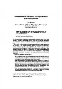
All scenarios involve the body bus CAN network of Fig. 1 (i.e., with 4 nodes) with 9 messages (4 event messages and 5 periodic messages). It is assumed that the assignment of priorities to event messages and periodic messages is arbitrary and likewise the assignment of messages to nodes is also arbitrary. The scenarios basically result from a specific assignment of message priorities and another specific assignment of messages to nodes. For Scenario 1 depicted in Fig. 2, the priority of event messages per node is higher than the priority of periodic messages assigned to the same node. However, on the overall network basis, it is possible that the priorities of some event messages are lower than the priority of some other periodic messages. Message priorities are also independent from nodes, i.e.; any node can have messages of any priority level. Scenario 2 (Fig. 3) is similar to Scenario 1 with the additional limitation that messages in a certain priority range are collected and assigned to a certain node, thus in effect assigning priority levels to nodes even though the
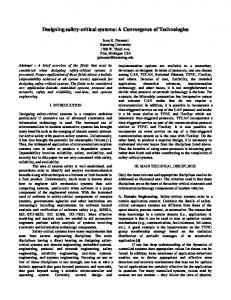
CAN protocol is based on message priorities rather than node priorities. For Scenario 3 (Fig. 4) we will assume the basic configuration of Scenario 1 except that all event messages have higher priority than the periodic messages.
contrast, message priorities in Scenarios 2 and 3 must comply with the order depicted in Figs. 2 and 4. The main advantage (that is not obvious) of some configurations over others is that the message latencies can be optimized if some rules for assigning message priorities and assigning messages to nodes are followed. This is proved later in this paper. Other scenarios
READY MESSAGES IN PRIORITY ORDER
e1
BUS TRANSMIT BUFFER Node 1
e1 e20
Node 2 READY MESSAGES IN PRIORITY ORDER
e3 0
p51
Other important practical considerations that have an impact on performance have not been considered in this paper because it is beyond its scope. These include the effects of transmission errors due to external interference’s, and failures in systems with redundant components.
Node 3
e1 e1
p60
BUS TRANSMIT BUFFER Node 1
0
p70
Node 4
p80
e20
Node 2
e3 0
p51
p100 SPORADIC MESSAGE PERIODIC MESSAGE
Node 3
p60 p70
Node 4
p80 Fig. 2. CAN network where message priorities are independent of nodes.
Performance In this paper we are primarily interested in message latency (or message delay) as the main indicator of performance. For the purpose of this paper we define message latency as the time interval between the instance when a message is ready for transmission and queued at a transmitting node until the message is successfully assembled at a receiving node. According to this definition, message latency includes the wait time at the transmission node, the time for the bus contention resolution, and the transmission time. Obviously, the performance of the configuration of Scenario 1 is different than that of the corresponding configurations of Scenarios 2 and 3. Scenario 1 is unconstrained and the designer is free to assign message priorities as he (or she) sees fit. In
p100 Fig. 3. CAN network where message priorities are defined by nodes.
Priority Inversion A priority inversion situation occurs, if on a certain node, a message with higher priority is ready to be transmitted and another message with lower priority is already pending in the Tx buffer of the same node. In this situation, the higher priority message has to wait until the low priority message is sent. This transmission may be delayed by other, mid-priority messages being sent by other nodes on the bus. In many cases, the Tx buffer register is empty, when a request for a new message transmission arrives. Let us illustrate an example of a bad situation using the scenario depicted in Fig. 4. Let us
assume that while the Tx buffer of node one has a pending message p100 (i.e., a periodic message with priority 100), a new event message e1 arrives at Node 1 followed by e20. Note that e1 has Priority 1, the highest priority assumed in this paper. All other nodes (2 to 4) have messages with priorities ranging between 10 and 90 in their corresponding transmit buffers. Message p100 in node 1 has to wait until all other higher priority messages have been sent (6 messages). Then p100 is sent and then e1. This means that e1 has a delay equivalent to 8 messages times. The delay is the sum of all single transfer times for the corresponding messages. To complicate matters, additional messages with priorities between 1 and 100 may arrive at Nodes 2, 3, or 4 before message p100 has the chance to transmit, thus resulting in additional delays for e1. In the worst case, e1 has to wait forever, even though e1 is the highest priority message in the network! While the assumption about the already blocked Tx buffer for all nodes may be an excessive worst case situation; the possibility that Tx buffers are already blocked only for a subset of nodes may prove dangerous for critical applications involving safety. In this paper we analyze both extremes. READY MESSAGES IN PRIORITY ORDER
e1 e1
TRANSMIT BUFFER
prototype electric vehicle. Many of the signals have identical periods and have small message sizes ranging from 1 to 8 bits. To increase bus utilization, we assume that we can combine the group of signals into a number of periodic messages making up the background load as listed in Table 1. We control the total bandwidth of the background load by varying the length and period of each of the messages. Table 1 lists the parameters for two example loads. Load A corresponds to a background load of 20.48% (i.e., they generate a total of 25600 Kbps) and a total background load (including overhead and bit stuffing bits) of 52000 Kbps (41.60 % of total bandwidth). We further assume that all simultaneous messages have a constant message length of 2 bytes. In Section 4, we will analyze the worst-case message latency when a number of event messages arrive simultaneously. Table 1. Two examples of background loads (Rate = 125 Kbps). Ld
P
Dm
T (ms)
Cm (ms)
OL Kpbs
TOL Kpbs
A
5
8
12.5
1.0448
25600 20.48%
52000 41.6%
B
8
2
16
0.584
8000 6.4%
36500 29.2%
BUS
Node 1
0
TIME TRIGGERED AND EVENT TRIGGERED ANALYSIS
e20 Node 2
e3 0
p51 Node 3
p60 p70 Node 4
p80 p100
As noted, time triggered analysis assumes that all messages are periodic and that event messages can be treated as periodic messages with the minimum interarrival time between messages as its period. Given this assumption, exact timing analysis can be performed on a CAN network subjected to periodic loads. An example of an analysis technique is that of Tindell et al. [1] where an algorithm is provided for calculating message latencies on CAN networks. Appendix A contains a summary of the algorithm. Provided that the message traffic is schedulable (the latency calculations converge or the network can satisfy the requirements of the offered load) the analysis is said to be deterministic. This is so because a specific procedure is known for calculating message latencies for all messages and the latency values are unique and bounded. Problems with time-triggered analysis
Fig. 4. CAN network where message priorities are higher for event messages.
We configure the background load as a load benchmark for the body bus network similar to the “SAE Benchmark” reported in [1]. The benchmark corresponds to many typical signals (53 in the SAE benchmark) in a
The main problem with the time triggered analysis approach, is that it cannot deal with event messages accurately. Another related problem is that it cannot deal with simultaneous or concurrent events. Theoretically two or more simultaneous events can occur at the same time, but no network can handle a system with an arbitrary number of such simultaneous events. In practice,
systems are designed to handle those concurrent events that have a specified minimum inter-arrival time. For some body bus networks a value of a minimum interarrival time is typically 20 ms. Thus, time triggered analysis alone is not sufficient to accurately evaluate message latencies involving event messages in applications. In this paper we use combined time and event triggered analysis, thus overcoming the principal disadvantage of the time triggered analysis approach, that of handling event messages. By definition, event messages occur whenever they are generated by an application which occur on a random basis (e.g., one does not know the precise instant when an event generated by a passenger rolling a window up or down occurs). Thus, the analysis of event messages is nondeterministic in that a specific procedure may or may not be known for calculating message latencies for all messages and the latency values are not unique but rather they are random. It follows that the analysis involving a combined network load of periodic and event based messages is also non-deterministic. This is perhaps the main reason why many analysis methods use time triggered analysis instead of a combined approach involving time triggered and event triggered analysis [4].
DESIGN PROCESS USING EVENT TRIGGERED ANALYSIS We assume a network such as that depicted in Fig. 1 with each node having a Tx buffer holding the message to be transmitted next. Other ready messages are waiting at each node, and whenever the Tx buffer becomes empty, the highest priority ready message will move into the empty Tx buffer and contend for the bus according to the CAN protocol. Thus, priority inversion is possible. Each node can generate periodic and simultaneous messages. We assume that a finite number of ne event messages are generated simultaneously. Unlike previous design processes available in the literature, in this paper we propose a design process that is centered on event triggered analysis. The main idea of the process is to begin with the main requirement that we have ne simultaneous messages in addition to a certain number of np periodic messages that constitute the background load. The design process involves solving two related sub-problems: I.
II.
The calculation of the maximum number simultaneous event messages for a given level background load, and The calculation of the maximum level background load for a given number simultaneous event messages.
of of of of
The solution of these two problems involve scheduling all the messages (periodic and simultaneous) over the CAN
network. Scheduling messages for transmission is done efficiently using message latencies as performance indicators. In addition, network bus utilization needs to be taken into account to detect an upper bound for the number of messages that can be scheduled. In the following we address each problem in turn. A. Calculating the maximum number of simultaneous messages. The idea is to schedule the given background (periodic) load first followed by simultaneous messages being added one at a time. After each simultaneous message is added, both the maximum (i.e., worst case) message latency and the current bus utilization is calculated. The process is terminated whenever a limit for a desired message latency or the maximum bus utilization (i.e., Bu = 1) is reached, whichever occurs first. B. Calculating the maximum level of background load for a given number of simultaneous event messages. The idea is the same as the previous method in A above, with the exception that the simultaneous messages are scheduled first and the periodic messages are added one at a time.
In both cases, the maximum message latency is calculated by any analytical method (e.g., using the recursive formulas developed by Tindell et.al.). Let us consider the maximum message latency network (i.e., the value of message latency for the message with the highest latency) as the criterion to schedule additional messages. Using Scenario 3 (Fig. 4) presented in Section 2, we analyze the relative order of message transmission by the various nodes. At every step, the CAN contention group is made up of the set of messages currently in the Tx buffer of the respective nodes. For example, at Step 2, the contention group = {p100,e10,p70,p80}. The winner in this group is e10, which is denoted by an * in Table 2. At every step, one message is sent over the CAN bus and deleted from the corresponding row. The last two rows of Table 2 contain the actual order of transmission and a rearranged set of messages for the purpose of worst-case message latency calculations. The rearranged set of messages makes up a rearranged set in such a way that all periodic messages in the set are transmitted first.
It can be noticed that, as a group, the statistical properties of the rearranged set are equivalent than the original set. More specifically, assuming that the message lengths for periodic and event messages are the same, the original set has an actual delay = {2,4,8,9} of units of message transmission times with mean and maximum values of 5.7 and 9 respectively. The rearranged set has delays = {6,7,8,9} with mean and maximum values of 7.5 and 9. There are advantages to reordering messages before making message latency calculations. First, priority inversion is taken into account; second, message latency calculations are simplified; and third, as far as worst case
latency calculations is concerned, the statistical properties of the rearranged set is the same as that of the original set. Thus the worst-case calculations on the rearranged set continue to be the worst case. However, the actual message latencies for any message depends on the actual values of priorities assigned to messages and the allocation of messages to nodes. Table 2. Evolution of messages at each node. Node 1
Node 2
Node 3
Node 4
Step 1 P100,e1,e20 p51*,e10 p70,e30 p80, p60 2 P100,e1,e20 e10* p70,e30 p80, p60 3 P100,e1,e20 --p70*,e30 p80, p60 4 P100,e1,e20 --e30* p80, p60 5 P100,e1,e20 ----p80*, p60 6 P100,e1,e20 ----p60* 7 P100*,e1,e20 ------8 e1*,e20 ------9 e20* ------Original order: p51,e10, p70,e30,p80,p60,p100,e1,e20 Rearranged order: p51,p60 p70,p80,p100,e1,e10,e20, e30 * Denotes the message with the highest priority in the contention group.
APPLICATIONS TO NETWORK ANALYSIS AND DESIGN To illustrate the process, let us consider the problem of calculating the maximum number of simultaneous messages that can be added to Load B of Table 1 (8 periodic messages each with 2 bytes, T = 16 ms, 6.4 % offered load, 0.292 bus utilization at 125 Kbps.). The terminating condition for the process is an upper limit to simultaneous message latencies of 16 ms (in this case equal to the period of the periodic messages). As outlined in the approach, we calculate the message latencies for the periodic messages and then the corresponding latencies for the simultaneous event messages. Table 3 shows the results of the calculations assuming that all event messages em have a length of 8 bytes. The maximum number of simultaneous messages is 9. Table 4 shows that the maximum number of simultaneous messages that can be sent are 11, 13, and 17 if we change the length of simultaneous messages to 6, 4, and 2 bytes respectively. Fig. 5 depicts the probability that message latency for a simultaneous message is less than a value of deadline. SUMMARY AND CONCLUSIONS A process for designing CAN-based distributed applications involving event triggered analysis has been presented. The process takes into account priority
inversion, a situation that occurs in practical implementations of the CAN protocol involving a transmit buffer to hold the pending message. For worst-case message latency calculations, message latencies in an actual network are the same as those in an equivalent network where the order of message transmission on the CAN bus has been re-arranged. The main advantage of the rearranged network is that the latency calculations are simplified. Message latencies of simultaneous messages depend on their order of arrival relative to messages in the background load, their priority, and the distribution of priorities across all nodes. It is possible to optimize the worst case message latencies of simultaneous messages by carefully assigning message priorities in such a way that priority inversion is minimized. The process involves the calculation of the maximum number of simultaneous event messages for a given level of background load and the calculation of the maximum level of background load for a given number of simultaneous event messages. Once the maximum number of simultaneous events and the maximum allowed message latency is known for a system, a developer can easily determine the appropriate mix of time-triggered and event triggered traffic that the network can sustain. Table 3. Message latencies of periodic messages followed by simultaneous messages. Message Length dm Period Latency (ms) (bytes) Tm (ms) pk 2 16 1.6288 pk-1 2 16 2.2128 pk-2 2 16 2.7968 pk-3 2 16 3.3808 pk-4 2 16 3.9648 pk-5 2 16 4.5488 pk-6 2 16 5.1328 pk-7 2 16 5.7168 em 8 NA 6.7616 em-1 8 NA 7.8064 em-2 8 NA 8.8512 em-3 8 NA 9.896 em-4 8 NA 10.9408 em-5 8 NA 11.9856 em-6 8 NA 13.0304 em-7 8 NA 14.0752 em-8 8 NA 15.12 em-9 8 NA 16.1648 em-10 8 NA 17.2096 NA: not applicable. Table 4. Maximum numbers of simultaneous event messages over a background load of 29.20% on a network with a rate of 125 Kbps. Message Transmission Max. # of length time @ 125 simultaneous event (bytes) Kbps messages (M) 8 1.0448 9
6 4 2
0.8912 0.7376 0.584
11 13 17
Email:
[email protected]
ACRONYMS, ABBREVIATIONS
REFERENCES
CAN: Controller area network.
[1] K. Tindell, and A. Burns, Guaranteeing message latencies on controller area network (CAN), 1st International CAN Conference, ICC’94, 1994.
Ld: Load P: Messages per load T: Period Cm: Transmission time dm: Message size OL: Offered load TOL: Total offered load
[2] K. Tindell, and J. Clark, Holistic Schedulabiltiy Analysis for Distributed Hard Real-Time Systems, Microprocessors and Microprogramming, March 1994. [3] K. Tindell, A. Burns, and A.J. Wellings, Calculating controller area network (CAN) message response times, Control Eng. Practice, 3(8): 11-63-1169, 1995. [4] N. Navet, Y.-Q. Song, and F. Simonot, Worst Case Deadline Failure Probability in Real-Time Applications Distributed over CAN, Journal of Systems Architecture, 46(7), 2000.
APPENDIX The following is a summary of the method given in [3]. A message m can be delayed by higher priority messages and by a lower priority message that has already obtained the bus (this time period denoted as Bm is the transmission time of the largest lower priority message). Thus the worst case message latency Rm is given by, Rm = Cm + Jm + Im
(1)
Where Cm is the message transmission time of a message, Jm is the queueing jitter, and Im is the queueing delay referred to as interference time. Im is the longest time that all higher priority messages can occupy the bus plus Bm, thus
Imn
Fig. 5. Probability distribution of simultaneous message latencies in terms of deadlines. M = number of simultaneous messages.
CONTACT Dr. Juan Pimentel is a Professor of Computer Engineering at Kettering University. He holds a Ph.D. degree in Electrical Engineering from the University of Virginia. Dr. Pimentel has done extensive research in the U.S, Germany, Spain, and Colombia. He is a Fulbright Scholar and an associate editor of the IEEE Transactions on Industrial Electronics and the Transactions on Mobile Computing. His main research areas are: distributed embedded systems, real-time networks and protocols, dependable systems, and electric propulsion systems. He is a member of Tau beta pi, Eta kappa nu, Sigma xi, IEEE, and SAE.
I mn + J j + τ b = Bm + Cj Tj ∀j∈hp(m)
∑
(2)
Where hp(m) is the set of messages of higher priority than m and Tj is the message period. The superscript n on Im denotes that it is a difference equation that needs to be solved starting with an initial value of 0 until convergence. The transmission time of a message Cj is given by, Cj = [ (34+8dj)/5 + 47 + 8dj]t b
(3)
Where dm is the message size and t b is the time to transmit one bit on the bus (on a bus running at 1 Mbit/sec this is 1 µs). In (), the term 47 is the size of the fixed-form but fields of the CAN frame and (34 + 8dm)/5 is the maximum number of stuff bits.