Modeling the scalar wave equation with Nyström methods

GEOPHYSICS, VOL. 71, NO. 5 共SEPTEMBER-OCTOBER 2006兲; P. T151–T158, 7 FIGS. 10.1190/1.2335505

Modeling the scalar wave equation with Nyström methods

Jing-Bo Chen1

To form a unified viewpoint and facilitate our understanding of numerical simulation schemes, we will accept that all numerical modeling schemes can be obtained by the second approach to discretization. Therefore, to construct modeling schemes for the scalar wave equation, we can first discretize space by finite-difference methods, pseudospectral methods, or finite-element methods. Second, we numerically integrate the resulting system of ordinary differential equations by discretizing time. Note that the obtained system of ODEs is of second order. When numerically solving this system directly, we need to approximately evaluate additional starting values in addition to initial values. The higher the order of the schemes, the more complex the evaluation of the additional starting values. Nyström methods are numerical methods designed for secondorder differential equations. Nyström 共1925兲 first considered this as a simplification of Runge-Kutta methods. Hairer et al. 共1993兲 systematically developed Nyström methods. There are two benefits in using Nyström methods. First, we do not need to evaluate the additional starting values. Second, by introducing an intermediate variable, the scalar wave equation can be cast into a Hamiltonian system. Using Nyström methods, we can develop the corresponding symplectic methods. The symplectic methods have remarkable capability for long-time computations. This is because the symplectic properties guarantee that the numerical solution evolves in the same system as the solution of the original continuous differential equation 共Feng, 1993; Sanz-Serna and Calvo, 1994兲. In this paper, I present the pseudospectral method and explore high-order time discretizations. I follow this with a discussion of Nyström methods. I then develop a fourth-order symplectic Nyström method with pseudospectral spatial discretization. Finally, I illustrate the performance of this scheme with numerical experiments that compare it with a second-order scheme and a fourth-order nonsymplectic Nyström method.

ABSTRACT High-accuracy numerical schemes for modeling of the scalar wave equation based on Nyström methods are developed in this paper. Space is discretized by using the pseudospectral algorithm. For the time discretization, Nyström methods are used. A fourth-order symplectic Nyström method with pseudospectral spatial discretization is presented. This scheme is compared with a commonly used secondorder scheme and a fourth-order nonsymplectic Nyström method. For a typical time-step size, the second-order scheme exhibits spatial dispersion errors for long-time simulations, while both fourth-order schemes do not suffer from these errors. Numerical comparisons show that the fourth-order symplectic algorithm is more accurate than the fourth-order nonsymplectic one. The capability of the symplectic Nyström method in approximately preserving the discrete energy for long-time simulations is also demonstrated.

INTRODUCTION Seismic modeling is an important foundation of exploration seismology. High-accuracy seismic modeling schemes are increasing in demand as computing capacity increases. In this context, high-accuracy schemes are developed using Nyström time-stepping methods and pseudospectral spatial discretizations. Numerical schemes for modeling of the scalar wave equation involve discretizations of both space and time. This discretizing process can be accomplished in two ways. The first way is to discretize both space and time simultaneously. The finite-difference methods 共Claerbout, 1985兲 belong to this category. The second way is first to discretize space to obtain a system of ordinary differential equations 共ODEs兲 with time as a variable and then to construct numerical schemes by discretizing time for the system of ODEs. The pseudospectral methods 共Gazdag, 1981兲 and the finite-element methods 共Ciarlet and Lions, 1991兲 fall into this second category.

PSEUDOSPECTRAL METHODS As mentioned above, we can use finite-difference methods, pseudospectral methods, or finite-element methods for the space discretization. I use pseudospectral methods, for which the errors result

Manuscript received by the Editor July 18, 2005; revised manuscript received February 6, 2006; published online September 5, 2006. 1 Chinese Academy of Sciences, Institute of Geology and Geophysics, P.O. Box 9825, Beijing 100029, China. E-mail: [email protected]. © 2006 Society of Exploration Geophysicists. All rights reserved.

T151

T152

Chen

mainly from the time discretization. For higher accuracy, we need higher-order time discretization. The issue of computing additional starting values becomes more evident in this situation. Pseudospectral methods for modeling of the scalar wave equation were presented by Gazdag 共1981兲. The main point of the pseudospectral methods is to express the wavefield under consideration in terms of a complete set of orthogonal basis functions whose derivatives are known exactly. In practice, Fourier pseudospectral methods are usually employed. Consider the scalar wave equation

冉

冊

2 ⳵ 2u ⳵ 2u ⳵ 2u 2 ⳵ u + 2 , 2 = c 2 + ⳵t ⳵x ⳵y2 ⳵z

共1兲

where u共x,y,z,t兲 is the wavefield and c共x,y,z兲 is the velocity. Let u = 关u1,1,1, . . ., uNx,Ny,Nz兴T, where T represents transpose and ui,j,l are the wavefield values at discrete locations, i.e., ui,j,l ⬇ u共i⌬x, j⌬y, l⌬z,t兲; i = 1, . . ., Nx; j = 1, . . ., Ny; l = 1, . . ., Nz. The values ⌬x, ⌬y, and ⌬z are grid increments in the x-, y-, and z-directions; and Nx, Ny, and Nz are the number of grid lines in the x-, y-, and z-directions, respectively. The semi-discrete system resulting from the pseudospectral method for equation 1 is

d 2u = c2F −1关w ⴱ F共u兲兴, dt2

共2兲

where F and F −1 represent 3D forward and inverse finite Fourier transforms, respectively, and w = 关w1,1,1, . . ., wNx,Ny,Nz兴T with wi,j,l = −共kx2i + k2y j + kz2l兲, where kxi, ky j, and kzl are discrete wavenumbers in the x-, y-, and z-directions, respectively. The asterisk ⴱ denotes array multiplication between vectors. For example, suppose that p = 共p1,p2, . . ., pm兲 and q = 共q1,q2, . . ., qm兲, then p ⴱ q = 共p1q1,p2q2, . . ., pmqm兲. To obtain the final modeling scheme, we further discretize equation 2 in time. A standard second-order time difference is often used and gives

u共t0 + 2⌬t兲 = 2u共t0 + ⌬t兲 − u共t0兲 + c F 关w ⴱ F共u共t0 + ⌬t兲兲兴⌬t , 2

−1

2

共3兲

where ⌬t is the time-step size and t0 is the initial time. As usual, we take t0 = 0. To compute u共2⌬t兲 using equation 3, we need to know u共0兲 and u共⌬t兲, which can be computed from the initial conditions of equation 1: u共0兲 and ⳵u共0兲/⳵t. We can evaluate u共0兲 directly from u共0兲. To obtain u共⌬t兲, a third-order scheme based on a Taylor series expansion was given by Gazdag 共1981兲 as 3

u共⌬t兲 =

兺 i=0

⳵iu共0兲 共⌬t兲i . i! ⳵ti

共4兲

In equation 4, u共0兲 and ⳵u共0兲/⳵t are known, ⳵2u共0兲/⳵t2 is defined by equation 1, and ⳵3u共0兲/⳵t3 is obtained by

冉

2 ⳵ 3u ⳵2 ⳵2 2 ⳵ = c + + ⳵t3 ⳵x2 ⳵ y 2 ⳵z2

冊冉 冊

⳵u , ⳵t

which is obtained by substituting ⳵u/⳵t for u in equation 1. Finally, we can compute u共⌬t兲 directly from u共⌬t兲. The main error in scheme 共equation兲 3 is associated with the time differencing. Thus, to improve accuracy, we need to use a higher-

order time difference. A natural choice is the fourth-order time difference

u共4⌬t兲 = 16u共3⌬t兲 − 30u共2⌬t兲 + 16u共⌬t兲 − u共0兲 − 12c2F −1关w ⴱ F共u共2⌬t兲兲兴⌬t2 .

共5兲

However, we can show that scheme 5 is unconditionally unstable by using the standard spectral analysis. Using the Taylor series and the wave equation, another approach for high-order time differencing was presented by Etgen 共1986兲. But this approach still requires the computation of additional starting values. For example, for a fourthorder method, we need a fifth-order scheme to compute the starting values instead of the third-order scheme 4. We are faced with a cumbersome procedure for computing starting values. Therefore, an alternative approach is needed.

NYSTRÖM METHODS The basic idea of Nyström 共1925兲 methods is as follows: First introduce an intermediate variable to reduce the second-order wave equation to an equivalent first-order system; then apply Runge-Kutta methods to the first-order system and simplify by taking advantage of the special form of the first-order system. The obtained Nyström methods do not need to evaluate starting values and have considerably less computational cost than Runge-Kutta methods applied directly to the first-order system for second-order equations such as equation 2. For details, refer to Hairer et al. 共1993兲. For our purposes, consider a second-order system of ordinary differential equations written in the form

d 2y = f共y兲. dt2

共6兲

A Nyström method for system 6 reads

冉

s

冊

Zi = f y0 + ci⌬tz0 + ⌬t2 兺 aijZ j , j=1

i = 1, 2, . . ., s,

s

y1 = y0 + ⌬tz0 + ⌬t

2

¯b Z , 兺 i i i=1

s

z1 = z0 + ⌬t 兺 biZi ,

共7兲

i=1

where z = dy/dt, y0 = y共0兲, z0 = z共0兲, y1 ⬇ y共⌬t兲, z1 ⬇ z共⌬t兲 and where ci, aij, ¯bi, and bi are constants that determine the order of the method. The numerical solution y1 is obtained through auxiliary variables Zi in scheme 7. The starting values y0 and z0 = dy共0兲/dt in scheme 7 are both known, and no additional starting values are needed. Scheme 7 requires computation of z1, but this is easy to accomplish because the main evaluations of Zi have been done previously in the computation of y1. The order conditions 共via the algebraic equations satisfied by ci, aij, ¯bi, and bi兲 have been obtained by using tree theory in Hairer et al. 共1993兲. By solving these algebraic equations, we can obtain the corresponding methods. Consider a stable fourth-order explicit method 共Qin and Zhu, 1991兲:

Modeling with Nyström methods

c1 =

3 + 冑3 , 6

c2 =

冑 ¯b = 5 − 3 3 , 1 24

3 − 冑3 , 6

c3 =

冑 ¯b = 3 + 3 , 2 12

b1 =

3 − 2冑3 , 12

b2 =

a21 =

2 − 冑3 , 12

a32 =

6

methods. Therefore, Nyström methods can be applied directly. We introduce a variable v = du/dt and apply Nyström method 8 to equation 2 to obtain

冑 ¯b = 1 + 3 , 3 24

1 , 2

冑3

3 + 冑3 , 6

b3 =

冋 冉 冋 冉 冋 冉

3 + 2 冑3 , 12

,

3 + 冑3 ⌬tv0 6

V2 = c2F −1 w ⴱ F u0 +

3 − 冑3 2 − 冑3 2 ⌬tv0 + ⌬t V1 6 12

V3 = c2F −1 w ⴱ F u0 +

冑3 2 3 + 冑3 ⌬tv0 + ⌬t V2 6 6

u1 = u0 + ⌬tv0 + ⌬t2

With these coefficients, scheme 7 becomes

冊

Z1 = f y0 +

3 + 冑3 ⌬tz0 , 6

Z2 = f y0 +

3 − 冑3 2 − 冑3 2 ⌬tz0 + ⌬t Z1 , 6 12

Z3 = f y0 +

冑3 2 3 + 冑3 ⌬tz0 + ⌬t Z2 , 6 6

y1 = y0 + ⌬tz0 + ⌬t2 +

冊

1 + 冑3 Z3 , 24

z1 = z0 + ⌬t

冉

冉

+

冊

冊

冊

3 + 2冑3 3 − 2冑3 1 Z1 + Z2 + Z3 . 12 2 12

共8兲

Another benefit of Nyström methods is that we can develop symplectic algorithms if equation 6 possesses a symplectic structure. In the past, we only focused on the accuracy of the numerical methods when solving differential equations numerically. However, with the tremendous progress in computer technology and numerical analysis theory in recent decades, computation has become a third category of methods in scientific research in addition to theory and experiment. Not only is the accuracy of numerical methods expected, but structure-preserving properties also are required. Solutions to differential equations usually preserve various structures such as symplectic structure, multisymplectic structure, and various geometric structures. When solving differential equations numerically, some numerical methods also preserve these structures 共they are usually called structure-preserving algorithms兲, while others violate them. The structure-preserving methods have remarkable capability for long-time computation. The scalar wave equation 1 has a classical Hamiltonian structure 共Chen, 2004兲. Therefore, we can develop the corresponding structure-preserving methods 共see Appendix A兲.

A PSEUDOSPECTRAL METHOD WITH FOURTH-ORDER NYSTRÖM TIME DIFFERENCE Now we return to the issue of higher-order time difference for equation 2. Equation 2 is a second-order system of ordinary differential equations obtained from equation 1 by using pseudospectral

冊

冉

,

5 − 3冑3 3 + 冑3 V1 + V2 24 12

1 + 冑3 V3 , 24

v1 = v0 + ⌬t

5 − 3冑3 3 + 冑3 Z1 + Z2 24 12

冊册

V1 = c2F −1 w ⴱ F u0 +

a11 = a12 = a13 = a22 = a23 = a31 = a33 = 0.

冉 冉 冉

T153

冉

冊册

冊

3 − 2冑3 3 + 2冑3 1 V1 + V2 + V3 . 12 2 12

冊册

,

,

共9兲

Scheme 9 is a stable fourth-order explicit Nyström method with accuracy of O共⌬t4兲 共Qin and Zhu, 1991; Hairer et al., 1993兲. Because we use pseudospectral spatial discretization, the spatial accuracy is of exponential order O共exp共⌬x兲兲 共Fornberg, 1996兲. Therefore, the total accuracy of scheme 9 is O共⌬t4 + exp共⌬x兲兲.As pointed out by Hairer et al. 共1993兲, the Nyström method 共scheme 9兲 is considerably more efficient than Runge-Kutta methods. In seismic modeling based on scheme 9, we compute u1 and v1 from known u0 and v0 = du0 /dt. Then we repeat this process with u0 and v0 replaced by u1 and v1, respectively. Higher-order Nyström time differences are easily available, and they have the same format as scheme 9 but with more Vis.

NUMERICAL EXPERIMENTS In this section, we perform numerical experiments to test the feasibility and performance of the presented scheme. For clarity and simplicity, we only consider the 2D case. As in Gazdag 共1981兲, we use the initial conditions

u共x,z,t = 0兲 = exp关− 0.0001共x2 + 共z − z0兲2兲兴 and

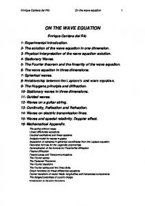
⳵u共0兲 = 0. ⳵t The grid increments are ⌬x = ⌬z = 50 m. Here, z0 is a constant that indicates the position of the source. In the following numerical examples, we use periodic boundary conditions. In the first example, we use scheme 9 to simulate wave propagation in a heterogeneous medium. The velocity model 共Figure 1兲 consists of three layers with velocities c = 1000 m/s, 2000 m/s, and 3000 m/s; a straight interface; and a curved interface. The source is set at 共x = 0 m, z = 200 m兲. The time-step size ⌬t is 0.006 s. Figure 2 shows the wavefield at t = 0, 0.438, 0.936, 1.248, 1.56, and 1.872 s. The simulated reflection and transmission phenomena are qualitatively correct.

T154 We now make numerical comparisons between scheme 9 and the commonly used scheme 3. In this example, we use the velocity c = 3000 m/s and the time step size ⌬t = 0.006 s. The starting value for equation 3 is computed through equation 4, which requires evaluating the second-order spatial derivatives of the initial conditions. Therefore, when using schemes like equation 3 in wave simulation, we usually require that the initial conditions have a certain degree of smoothness, which sometimes is not satisfied in practice 共for example, discrete initial conditions兲. In contrast, when using scheme 9, we

Figure 1. The velocity model used for the numerical experiments. It consists of three layers with velocities c = 1000 m/s, 2000 m/s, and 3000 m/s, respectively; a straight interface; and a curved interface.

Chen have no special requirement on the initial conditions, which makes schemes like 9 more practical. In Figure 3, we show the impulse responses for schemes 3 and 9 after 200, 500, and 5000 time steps, respectively. For time steps equal to or less than 200, impulse responses for both schemes 3 and 9 do not exhibit spatial dispersion errors. After 500 time steps, the spatial dispersion becomes evident in the wavefront computed with scheme 3, which contrasts with the clean wavefront computed with scheme 9 共Figure 3c and d兲. After 5000 time steps 共t = 30 s兲, the wavefront computed with scheme 3 has blurred very badly, but the wavefront computed with scheme 9 is still sharp 共Figure 3e and f兲. These observations indicate that for a typical time-step size of 0.006 s, the commonly used scheme 3 is not suitable for lengthy simulations. Now we perform simulations by scheme 3 with smaller time-step sizes of 0.004, 0.003, 0.002, and 0.001 s. To compute the wavefront at 30 s, the number of time steps is 7500, 10,000, 15,000, and 30,000, respectively. Figure 4 shows the simulation results. We see that dispersion errors decrease as time-step size decreases. The result with time-step size of 0.001 s is similar to that obtained with scheme 9 with a time-step size of 0.006 s 共Figure 3d兲. This indicates that to obtain the impulse response at 30 s, scheme 9 with a time-step size of 0.006 s is more efficient than scheme 3 with a time-step size of 0.001 s. We can explain this as follows: Although for each time step scheme 9 needs to compute three pairs of FFTs 共forward and inverse兲, which is three times as many as that of the scheme 3, the timestep size used in scheme 9 is six times as large as that used in scheme 3. Because the main computational cost in both schemes 9 and 3 is the computation of FFTs, the overall computational cost of scheme 9 is only half that of scheme 3. To demonstrate the advantages of the symplectic method, we now make numerical comparisons between the fourth-order symplectic Nyström scheme 9 with the following fourth-order nonsymplectic Nyström scheme:

V1 = c2F −1关w ⴱ F共u0兲兴,

冋 冉 冋 冉

V2 = c2F −1 w ⴱ F u0 +

1 1 ⌬tv0 + ⌬t2V1 2 8

V3 = c2F −1 w ⴱ F u0 + ⌬tv0 + u1 = u0 + ⌬tv0 + ⌬t2 v1 = v0 + ⌬t

Figure 2. Wavefield evolution with time computed with scheme 9. Distance and time are measured in meters and seconds, respectively.

冉

冉

1 2 ⌬t V2 2

冊 冊

冊册

冊册

,

,

1 1 V1 + V2 , 6 3

2 1 1 V1 + V2 + V3 . 6 3 6

共10兲

Figure 5 shows the impulse response computed with scheme 10 after 5000 time steps. The time-step size is 0.006 s. We see that the result is similar to that computed with the symplectic scheme 9 共Figure 3f兲. To examine more closely the results obtained by these two fourth-order schemes, amplitude curves at a fixed point 共x = −1600 m, z = 1600 m兲 over the time near 30 s 共5000 time steps兲 are shown in Figure 6a. We see discrepancy in the amplitude curves computed by the two fourth-order schemes. In Figure 6b, another amplitude curve is added, which is computed by the nonsymplectic scheme 10 with a smaller time step size of 0.001 s. It can be seen that the amplitude curve computed by the symplectic scheme 9 with a time-step size of 0.006 s agrees well with the amplitude curve com-

Modeling with Nyström methods puted by the nonsymplectic scheme 10 with a smaller time-step size of 0.001 s. This indicates that the fourth-order symplectic algorithm scheme 9 is more accurate than the fourth-order nonsymplectic algorithm scheme 10 for the same time-step size. To show how the amplitude curves computed by the nonsymplectic scheme 10 with smaller time-step sizes approach the amplitude curve computed by the symplectic scheme 9 with a time-step size of 0.006 s, we plot the following amplitude-difference curves 共Figure 6c兲:

AD⌬t共t兲 = S0.006共t兲 − NS⌬t共t兲, where AD⌬t共t兲 denotes the amplitude-difference curve; S0.006共t兲, the amplitude curve computed by the symplectic scheme 9 with a timestep size of 0.006 s; and NS⌬t共t兲, the amplitude curve computed by the nonsymplectic scheme 10 with a time-step size of ⌬t. Here we take ⌬t = 0.006, 0.004, 0.002, and 0.001 s. We can see that the magnitude of the curves of the amplitude difference diminishes with decreasing ⌬t. From the above numerical comparisons, we can conclude that to achieve approximately the same accuracy, the symplectic algorithm scheme 9 is much more efficient than the nonsymplectic algorithm scheme 10, considering the time-step sizes used. This is a great advantage.

T155

Another important advantage of a symplectic algorithm is its ability to approximately preserve energy for lengthy simulations 共Feng, 1993; Sanz-Serna and Calvo, 1994兲. For the wave equation utt = c2共uxx + uzz兲 with a periodic boundary condition, the true solution preserves the energy

冕

M

共v2 + c2共u2x + uz2兲兲dxdz,

where v = ut and M is the integral domain. Now in our numerical experiments, we monitor the discrete energy

G共n兲 =

兺 i,l

冋

+ c2

n 2 共vi,l 兲 + c2

冉

冉 冊 冊册

n n ui,l+1 − ui,l ⌬z

n n − ui,l ui+1,l ⌬x

2

2

⌬x⌬z,

Figure 4. Impulse response at 30 s. The results are computed with scheme 3 with time-step sizes of 0.004, 0.003, 0.002, and 0.001 s, respectively.

Figure 3. Impulse responses computed with schemes 3 and 9. 共a兲 and 共b兲 200 time steps; 共c兲 and 共d兲 500 time steps; 共e兲 and 共f兲 5000 time steps. Views 共a兲, 共c兲, and 共e兲 are computed with scheme 3; 共b兲, 共d兲, and 共f兲 are computed with scheme 9.

Figure 5. Impulse response after 5000 time steps computed with scheme 10 with a step-time size of 0.006 s.

T156

Chen

Figure 7. Discrete energy curves 关G共n兲 versus n兴 for the symplectic scheme 9 and the nonsymplectic scheme 10. 共a兲 N = 5000; 共b兲 N = 100,000. half of the energy is lost in the energy curve for the nonsymplectic scheme 10. This demonstrates the capability of the symplectic algorithm for approximately preserving the discrete energy for lengthy computations.

CONCLUSIONS

Figure 6. Amplitude and amplitude-difference curves at a fixed point 共x = −1600 m, z = 1600 m兲 over the time near 30 s. 共a兲 Amplitude curves computed by the symplectic scheme 9 with ⌬t = 0.006 s 共blue line兲 and the nonsymplectic scheme 10 with ⌬t = 0.006 s 共red line兲. 共b兲 Amplitude curves computed by the symplectic scheme 9 with ⌬t = 0.006 s 共blue line兲; the nonsymplectic scheme 10 with ⌬t = 0.006 s 共red line兲; and the nonsymplectic scheme 10 with ⌬t = 0.001 s 共green line兲. 共c兲 Amplitude-difference curves: ⌬t = 0.006 s 共red line兲; ⌬t = 0.004 s 共blue line兲; ⌬t = 0.002 s 共yellow line兲; and ⌬t = 0.001 s 共green line兲. n n where vi,l ⬇ v共i⌬x,l⌬z,n⌬t兲, ui,l ⬇ u共i⌬x,l⌬z,n⌬t兲, and n = 0,1,2, . . ., N. Here, N is the number of time steps. Figure 7a shows the discrete energy curves 关G共n兲 as a function n兴 for both schemes 9 and 10, with N = 5000. For the symplectic scheme 9, the energy curve fluctuates about a constant energy. For the nonsymplectic scheme 10, a numerical loss in energy is observed. The corresponding result for N = 100,000 is shown in Figure 7b. For this very long computation, the energy curve for the symplectic scheme 9 still fluctuates about a constant energy while nearly

Nyström time differencing with pseudospectral spatial discretizaiton is presented for modeling of the scalar wave equation. Two fourth-order Nyström schemes with pseudospectral spatial discretizaiton are developed; one is symplectic and the other is nonsymplectic. Numerical experiments demonstrate three results. First, these fourth-order schemes can be used for long-time simulations with a time-step size of 0.006 s, whereas the commonly used second-order scheme exhibits severe dispersion errors for this computation time and time-step size. Second, the fourth-order schemes with a timestep size of 0.006 s are more efficient than the second-order scheme with a small time-step size of 0.001 s. And third, the symplectic algorithm is more accurate than the nonsymplectic algorithm and has a better capability of approximately preserving the discrete energy for lengthy simulations. Preserving propagation energy is only one feature of preserving symplectic structure. The symplectic algorithms also have other features such as better accuracy, which can be explained by the theory of backward error analysis 共Hairer et al., 2002兲. According to this theory, the solutions of both symplectic and nonsymplectic algorithms for a Hamiltonian system formally satisfy a perturbed system.

Modeling with Nyström methods However, the perturbed system satisfied by the symplectic algorithms retains the Hamiltonian structure; the system satisfied by the nonsymplectic algorithms does not.

T157

du = v, dt dv = c2F −1关w ⴱ F共u兲兴. dt

共A-3兲

ACKNOWLEDGMENTS Further, we can reformulate equation A-3 as I would like to thank professor Arcone and anonymous reviewers for valuable suggestions and corrections, that led to a great improvement of this paper. This work is supported by the National Natural Science Foundation of China under grant 40474047 and also partially by the Chinese Academy of Sciences with Key Project of Knowledge Innovation KZCX1-SW-18.

冋册 冋 册

d u dt v

=

0

I

−I 0

冤冥

⳵H ⳵u , ⳵H ⳵v

共A-4兲

1

where I is an identity matrix and H = 2 关vTv + c2uTDu兴. The matrix D is a second-order spectral differential matrix which satisfies

APPENDIX A HAMILTONIAN STRUCTURE In this appendix, I present the Hamiltonian structure and the corresponding symplectic algorithms for the scalar wave equation. Introducing an intermediate variable v = du/dt, equation 1 is equivalent to

⳵u = v, ⳵t

冉

冊

⳵v ⳵ 2u ⳵ 2u ⳵ 2u + + . = c2 ⳵t ⳵x2 ⳵ y 2 ⳵z2

共A-1兲

冋册 冋 册 =

0

1

−1 0

⳵F ⳵F J ⳵ P0 ⳵ P0

冤冥

␦H ␦u , ␦H ␦v

共A-2兲

where

H=

1 2

冕冋

v2 + c2

冉冉 冊 冉 冊 冉 冊 冊册 ⳵u ⳵x

2

+

⳵u ⳵y

2

+

⳵u ⳵z

For details about spectral differential matrix, see Chen and Qin 共2001兲. Equation A-4 is a standard finite-dimensional Hamiltonian system. A finite-dimensional Hamiltonian system is just a system of ordinary differential equations that has the form of equation A-4. The true solution of equation A-4 preserves the symplectic structure du Ù dv. In other words, if we suppose that the solution of equation A-4 is P = F共 P0兲, where P = 关u,v兴T and P0 = 关u共t = 0兲,v共t = 0兲兴T, then the fact that F共 P0兲 preserves the symplectic structure du Ù dv is equivalent to F共 P0兲 satisfying

冋 册冋 册

Equation A-1 can be reformulated as

⳵ u ⳵t v

F −1关w ⴱ F共u兲兴 = Du.

2

dxdy

is the Hamiltonian system, and ␦ denotes the variational derivative. Equation A-2 is an infinite-dimensional Hamiltonian system. The evolution of the wavefield with time is characterized by a symplectic structure 兰du Ù dvdxdy, which can be viewed as an antisymmetric quadratic form. For the exact definition of symplectic structure, as well as the infinite-dimensional Hamiltonian system and variational derivative, see Olver 共1993兲. In solving equation A-2 numerically, we can use finite-difference, finite-element, or pseudospectral methods to discretize the space and obtain a finite-dimensional system. Equation 2, which is obtained with a pseudospectral method, can be cast into a finite-dimensional Hamiltonian system. First, introducing v = du/dt, we can rewrite equation A-2 as

T

= J,

where J =

冋 册 0

I

−I 0

.

Here, 关 ⳵F/⳵ P0兴 is the Jacobian of the vector-valued function F共 P0兲. A function satisfying the above equality is also called a symplectic mapping. Thus, it is concluded that the time evolution of the seismic wavefield is a symplectic mapping. In seismic modeling, we need to solve equation A-4 numerically. Suppose that ˜F共 P0兲 is the numerical solution of equation A-4 obtained by some numerical algorithm. Of course, the numerical solution ˜F共 P0兲 is the approximation of the true solution F共 P0兲. Does the numerical solution also have other properties? In fact, some numerical solutions are symplectic mappings while others are not. A numerical method is called a symplectic algorithm if the resulting numerical solution is a symplectic mapping. In the past, we mainly focused on the accuracy of the numerical solution to a Hamiltonian system; its structure-preserving properties were not considered seriously. With the introduction of symplectic algorithms and its great success in many physical fields, structurepreserving algorithms have developed into a very active and promising research area. The Hamiltonian framework developed here provides a basis for applying symplectic algorithms in seismic modeling. Based on this framework, we should develop numerical solutions of equation A-4 that are also symplectic mappings, i.e., symplectic algorithms. Various symplectic algorithms for Hamiltonian systems have been developed. We can directly apply the symplectic algorithms to equation A-4. Based on a finite-difference spatial discretization, Hamiltonian systems also can be obtained 共Luo

T158

Chen

et al., 2001兲. However, this kind of spatial discretization usually causes spatial dispersion errors. Now consider a Nyström formulation for equation A-4:

冋 冉

s

Vi = c2F −1 w ⴱ F u0 + ci⌬tz0 + ⌬t 2 兺 aijV j j=1

冊册

,

s

s

v1 = v0 + ⌬t 兺 biVi .

u1 = u0 + ⌬tv0 + ⌬t 2 兺 ¯biVi,

i=1

i=1

共A-5兲 If the coefficients in scheme A-5 satisfy

¯b = b 共1 − c 兲, i i i ¯ − a 兲 = b 共b ¯ bi共b j ij j i − a ji兲,

i = 1, . . ., s,

i, j = 1, . . ., s,

then scheme A-5 is a symplectic algorithm 共Sanz-Serna and Calvo, 1994兲. It is easy to check that the coefficients used in scheme 9 satisfy the above conditions; therefore, scheme 9 is a symplectic algorithm.

REFERENCES Chen, J. B., 2004, Multisymplectic geometry for the seismic wave equation: Communications in Theoretical Physics, 41, 561–566. Chen, J. B., and M. Z. Qin, 2001, Multisymplectic Fourier pseudospectral method for the nonlinear Schrödinger equation: Electronic Transactions on Numerical Analysis, 12, 193–204. Ciarlet, P. G., and J. L. Lions, 1991, Handbook of numerical analysis: NorthHolland. Claerbout, J. F., 1985, Imaging the earth’s interior: Blackwell Scientific Publications, Inc. Etgen, J. T., 1986, High-order finite-difference reverse migration with the two-way non-reflecting wave equation: SEP-48: Stanford University. Feng, K., 1993, The collected works of Feng Kang: Defence Industrial Press. Fornberg, B., 1996, A practical guide to pseudospectral method: Cambridge Univ. Press. Gazdag, J., 1981, Modeling of the acoustic wave equation with transform methods: Geophysics, 46, 854–859. Hairer, E., C. Lubich, and G. Warnner, 2002, Geometric numerical integration: Springer-Verlag, Berlin. Hairer, E., S. P. Nøsett, and G. Warnner, 1993, Solving ordinary differential equations I: Springer-Verlag, Berlin. Luo, M. Q., H. Liu, and Y. M. Li, 2001, Hamiltonian description and symplectic method of seismic wave propagation: Chinese Journal of Geophysics, 44, 120–128. Nyström, E. J., 1925, Über die numerische integration von differentialgleichungen: Acta Societe Scientiarum Fennicae, 50, 1–54. Olver, P. J., 1993, Applications of Lie groups to differential equations: Springer-Verlag, New York. Qin, M. Z., and W. J. Zhu, 1991, Canonical Runge-Kutta-Nyström methods for second order ODE’s: Computational Mathematics Applications, 22, 85–95. Sanz-Serna, J. M., and M. Calvo, 1994, Numerical Hamiltonian problems: Chapman and Hall.