Modeling Tumor/Polyp/Lesion Structure in 3D for Computer-Aided Diagnosis in Colonoscopy Chao-I Chena , Dusty Sargentb , Yuan-Fang Wanga a Dept.
of Computer Science, University of California, Santa Barbara, CA, USA 93106 b STI Medical Systems, 733 Bishop Street, Honolulu, HI, USA 96813 ABSTRACT
We describe a software system for building three-dimensional (3D) models from colonoscopic videos. The system is end-to-end in the sense that it takes as input raw image frames—shot during a colon exam—and produces the 3D structure of objects of interest (OOI), such as tumors, polyps, and lesions. We use the structure-from-motion (SfM) approach in computer vision which analyzes an image sequence in which camera’s position and aim vary relative to the OOI. The varying pose of the camera relative to the OOI induces the motion-parallax effect which allows 3D depth of the OOI to be inferred. Unlike the traditional SfM system pipeline, our software system contains many check-and-balance mechanisms to ensure robustness, and the analysis from earlier stages of the pipeline is used to guide the later processing stages to better handle challenging medical data. The constructed 3D models allow the pathology (growth and change in both structure and appearance) to be monitored over time. Keywords: Modeling, registration, visualization
1. DESCRIPTION OF PURPOSE Colorectal cancer, also called colon cancer, is the third most common form of cancer and the second leading cause of cancer-related death in the Western world. It can take many years for colorectal cancer to develop and early detection of colorectal cancer through regular screening greatly improves the chance of a cure. Among many screening techniques, colonoscopy is still considered the “gold standard” method. This research is aimed at developing the ability to construct 3D anatomic models of objects of interest (OOI, e.g., tumors, polyps, and lesions) from colonoscopic videos. These computer models can find many uses in a computer-aided diagnosis (CAD) system in colonoscopy to assist surgeons in visualization, surgical planning, and training.
2. METHOD Our method is based on the principle of structure-from-motion (SfM) in computer vision research. The SfM analysis uses the motion parallax effect—induced by varying the camera’s pose relative to the OOI—to deduce a 3D object’s depth (or structure). By combining the inferred 3D structure with the object’s appearance (color/texture) recorded in the video images, we arrive at a computerized 3D anatomic model. The flow chart of our system is depicted in Fig. 1. Different modules and their functions are described in more detail below.
2.1 Distortion Correction and Camera Calibration In video-endoscopy, difficulty in maneuvering the scope in a constricted body cavity results in large blind spots. Hence, endoscopic procedures often employ cameras using lenses of a short focus length, fisheye lens for example, to provide a large view volume. Such lenses cause significant distortion that degrades the accuracy of the constructed 3D models. Camera calibration is an offline process used to estimate the intrinsic parameters and to correct image distortion.1, 2 Figure 2(a) depicts fisheye distortion effect where straight lines have become barrelshape curves. Although clinicians may be accustomed to this type of distortion, it invalids many computer vision based analysis and model building algorithms. To over come this problem, distortion correction2 needs to be performed before any other image analyses. Figure 2(b) shows the corrected image. Further author information: (Send correspondence to Chao-I Chen) Chao-I Chen: E-mail:
[email protected], Telephone: 1 805 280 9655
Figure 1. System overview
(a)
(b)
Figure 2. Example of fish-eye lens distortion correction
(a)Original distorted image captured by a colonoscope (b)Corrected image
2.2 Feature Detection and Feature Matching A key requirement of the SfM analysis is to establish the precise camera poses in the video sequence. As no special tracking hardware, a magnetic tracker for example, is used in the conventional colon exam, the camera pose must be inferred from the input images alone. In computer vision, this inference process is accomplished by establishing 2D feature correspondences in multiple image frames. These corresponding 2D features in multiple images result from the projection of the same 3D entity. As incorrect, arbitrary camera poses generally will not produce the observed correspondence relations, it is possible to constrain the camera pose with enough such 2D correspondences. The 2D correspondence relationship can be produced by either continuous tracking or discrete matching. Continuous tracking techniques cannot easily deal with large motion blur, water or bubble injection, and strong glare reflection that are common in colonoscopic videos. Instead, we apply a SURF-based feature detector3 to detect locally invariant features in a few clean snapshots of the anatomy and match these features across multiple images to establish their correspondences. In contrast to the random drift shown over time by tracking methods, the SURF detector has been shown to provide very precise feature locations. This precision is crucial for the ensuing camera motion inference algorithm to accurately estimate the camera pose.
2.3 Outlier Filtering and Camera Motion Inference This step uses the matched 2D image features in two views to infer the camera’s movement in between the views. One crucial task is to eliminate outliers (mismatches). Although the classic RANSAC algorithm, one of the most widely used outlier filtering techniques, has been successfully applied to many applications, we found that the standard scheme does not always produce satisfactory results when applied to medical images. We therefore propose a two stage outlier filtering scheme to tackle challenging medical data. In the first stage, the normalized eight-point algorithm,4 together with a multi-RANSAC scheme, is performed to detect outliers. At the end of each RANSAC run, a fundamental matrix candidate F which encodes the camera movement information is generated. All feature correspondences that are correct (or compatible with ′ ′ this 3 by 3 matrix F ) should satisfy the equation p T F p = 0 where p and p are the point coordinates.1 A more intuitive error measure is to compute the squared sum of the Euclidean distances of the feature points from their corresponding epipolar lines. The point-line distances of both images are taken into account and the relation ′ ′ can be described by d(p , F p)2 + d(p, F T p )24 where function d(•, •) denotes the 2D Euclidean distance between the two arguments. Instead of setting a fixed threshold to detect outliers, we apply the box-plot method—a statistic method used to identify outliers without any assumption of the underlying data distribution—to automatically determine the outlier threshold. The box-plot method computes the lower quartile (the 25th percentile QL ) and the upper quartile (the 75th percentile QU ) of the data set. The difference between these two values (QU − QL ) is called the interquartile range or IQ . Any 2D feature with error distance larger than QU + 1.5 ∗ IQ is considered an outlier and is excluded from further computation. The process repeats until no outliers are detected. This multi-RANSAC scheme is motivated by one important observation — with the present of many outliers, the final model (the fundamental matrix in our application) suggested by the classic RANSAC algorithm is not a good description of the underlying data, but this semi-optimal result is good enough to help identify some outliers. After eliminating these outliers, more accurate model estimations can be expected in the next runs of RANSAC. It is also well known as the least-square principle that the more features we use to estimate a model the more likely the adverse effect of random Gaussian noise (in our case the noise causes slight, random perturbation to the 2D feature locations) can be averaged out during the computation. This is one of the reasons we propose to add a second stage process after the multi-RANSAC scheme. After outliers are removed from the feature list in the previous stage, all the remaining features then serve as input to an overdetermined five-point algorithm,5 a state-of-the-art algorithm for solving the relative camera pose problem. Furthermore, since the five-point algorithm’s outputs can be decomposed into the camera rotation (R) and translation (T ) parameters, we can locate feature points in 3D space through light-path triangulation. We use these 3D point positions to further filter out outliers in the second stage. As all 3D points should lie in front of the camera, whichever points that
Figure 3. Two-stage outlier filtering scheme
do not satisfy this constraint should be removed. This testing is referred to as identifying the cheirality of the 3D point cloud with respect to the camera.1 The whole procedure again is repeated a number of times until no more outliers are detected. Fig. 3 summarizes this two-stage scheme.
2.4 Bundle Adjustment Using Double Dog-Leg Method After all pairwise camera movement parameters have been computed, a nonlinear optimization method is applied to polish the estimated results from the previous step by minimizing the reprojection error. This optimization process is known as bundle adjustment that adjusts the bundle of rays between each camera center and the 3D point cloud.1 The camera motion parameters and the 3D point positions are adjusted simultaneously so that the rays intersect the cameras at locations as close as possible to all observed 2D features. We apply the Double Dog-Leg (DDL) algorithm,6 a trust-region method which intelligently combines the Gauss-Newton method and the gradient descent method. When employing a nonlinear optimization procedure, the convergence speed and the quality of the final solution are heavily influenced by the quality of the initial camera movement parameters and correctness of the 2D point correspondences. This was the reason why we proposed a sophisticated two stage outlier filtering method in section 2.3 to obtain a reliable initial guess. The way we employ the DDL to solve our problem is as follows: given a set of camera movement parameters, from a sequence of N image pairs, we parametrize rotation (R) and translation (T ) by 3 variables each in between two adjacent views. Because there is one global scale that should be shared by all partial structures, we take out one degree of freedom from one of the T vectors to ensure that this constraint is satisfied. That is, the direction of this particular T can change, but not its magnitude. The fixed magnitude enforces a fixed global scale. The resulting number of parameters is therefore 6N − 1 in total. We will see in section 2.7 how this global scale can be a great help for model registration.
2.5 Extended Polar Rectification The goal of this step is to rearrange image pixels so that the corresponding points (that result from the projection of the same 3D point) lie on the same image scan line. This configuration greatly reduces the search dimension (from 2D to 1D) of finding the point correspondences in the stereo matching analysis. Among many rectification algorithms, we chose the extended polar rectification due to its ability to handle all kinds of camera configurations, including two special cases: (1) the camera moves forward or backward (a common movement in colonoscopy) and (2) the camera experiences a pure side way motion. The extended polar rectification proposed by H¨ aming and Peters7 filled in details about how to use polar rectification when epipoles are at (or close to) infinity. Explicit thresholds and implementation details are described in their paper to detect extreme cases. Unlike Pollefeys’ polar rectification algorithm8 in which the orientation is determined using line homographies computed from the fundamental matrix or from the camera projection matrices, H¨ aming’s approach uses the fundamental matrix directly for orientation determination. We
Figure 4. Determine the orientation
will use Figure 4 as an example to demonstrate how fundamental matrix can be used directly to determine the orientation. Given an point x in image1, the epipolar line that passes through this point can be determined by computing the cross product of the point x and the epipole e. l =x×e
(1)
The corresponding epipolar line in image2 can also be determined though the fundamental matrix F and epipolar geometry. l′ = F x
(2)
Both line equations l and l′ separate the image planes into positive and negative regions. Given one correct pair of point correspondences, we can determine the sign s by making the following equation hold true. sign(l · p) = s · sign(l′ · p′ ) = s · sign((F x) · p′ )
(3)
Once the sign s is computed, the oriented fundamental matrix F o is equal to sF . Having the oriented fundamental matrix F o , the correct epipolar half-line can be easily determined. Now, for any given point x in the first image, a point x′ is considered to be on the correct epipolar half-line if the following equation hold true. sign((e × p) · x) = sign((F o p) · x′ )
(4)
2.6 Stereo Matching and Depth Inference A dynamic programming (DP)-based stereo matching algorithm9 is applied to establish point correspondence at each pixel in the input images. Once point correspondences are established, light-path triangulation is used to locate the actual 3D points and build a local model. Unlike traditional stereo matching algorithms using only rectified images as inputs, to improve the robustness we explicitly incorporate additional information and constraints derived from the previous steps to guide the stereo matching process. These constraints include clean features from the outlier filtering procedure and the camera motion parameters from the bundle adjustment procedure (Fig. 1). In more detail, given a set of reliable 2D point correspondences, we employ the Delaunay triangulation to partition the input images into small, localized regions. Furthermore, we explicitly examine the planarity hypothesis of these localized regions in the 3D space. To perform the planarity test robustly, adjacent triangles are first merged into larger polygonal patches and then the planarity assumption is verified. Once piecewise planar patches are identified, point correspondences within these patches are readily computed through planar homographies. These point correspondences established by planar homographies serve as the ground control points (GCPs) in the final DP-based stereo matching process. As Bobick proved in9 that GCPs not only improve the final results, but also speed up the matching process.
−13 −14 −15 −16 −17 −18 −19 −15 −10 −5 0 5
−10
−5
0
5
10
Figure 5. Results of constructing two point clouds using unified scale
Finally, we add a front propagation routine after some GCPs are established through homography computation to include more reliable GCPs. Our front propagation scheme works as follows: (1) Use all GCPs detected from the homography computation as seeds and (2) Perform a front propagation from these seeds until an edge or a predefined dissimilarity threshold is reached. The assumption is that the neighbors of a pair of reliable corresponding points are very likely to form corresponding pairs as well if these neighbors have similar intensity values and they are not located on the opposite sides of an object boundary. The threshold used to determine whether the difference between two pixels is small enough is a function of the distance between the current pixel’s coordinate and the coordinate of this pixel’s original seed point. Equation 5 describes how the threshold is computed at location x whose original seed point is s. threshold = (int)(255 ∗ e−(
dist(x,s) 2 ) σ
)
(5)
By adjusting the σ value in Equation 5, we can control the maximum allowed distance for any seed to propagate. Given any σ value, there is a corresponding minimum dist(x, s) which will make the computed threshold equals zero. In other words, after passing this distance, any pair of pixels can be considered a match only if these points’ intensity values are exactly the same. In reality, to enhance the robustness, intensity values are usually computed by applying sum of square distances (SSD) over small windows centered at these points. The chance for two non-correspondent points to have the same SSD values is small. We argue that this case only happens when the image intensity and color is homogeneous. Feature matching in homogeneous regions is considered a challenging, if not unsolvable, problem for all stereo algorithms.
2.7 Uni-scale Model Registration The final step is to register partial 3D models constructed from multiple two-view analyses into a more complete 3D model. Because a global scale had been determined during bundle adjustment, we treat each partial two-view model as a cloud of 3D points, and these point clouds are related by rigid-body transforms in space. To solve the registration problem, instead of applying the commonly used iterative closest point (ICP) algorithm10 which can be time consuming and error prone due to lack of point correspondences information, we solve a simple rigid-body transformation problem with the help of some reliable ground control points computed from 2D SURF features. The process is efficient, as we already have a good initial guess of the inter-frame camera movement from the previous steps. Please note that even with a consistent global scale, there are still a few point correspondences that do not locate closely in 3D space due to noise. Therefore, RANSAC is required when we estimate the rigid-body transformation parameters. Figure 5 depicts such case. Two 3D anchor points generated from real medical data are shown in this figure.
3. EXPERIMENTAL RESULTS We present some results using data from real colon examinations in this section. Fig. 6 summarizes some intermediate results of the two-view analysis. The leftmost figure in Fig. 6 shows a pair of rectified images where
Figure 6. Intermediate results of the two-view analysis: (Left to right) Rectified images, GCPs after planar homography computation, GCPs after the front propagation process and the final disparity map
Figure 7. (Left to right) One input image example, three sample depth maps using two-view analyses and the final depth map
the correspondent SURF features are connected by color lines. As the goal of rectification is to align epipolar lines with the images’ scan lines, corresponding features should lie horizontally. This is what we observed in Fig. 6 (with less than 0.5 pixel discrepancy in height). This high accuracy demonstrates the success of the sequence of routines described from section 2.1 to section 2.5. The other three figures from left to right in Fig. 6 depict detected GCPs using Delaunay triangulation and planar homographies, detected GCPs after the front propagation process, and the final disparity map with the diverticulum structure circled. After point correspondences are extracted from the disparity map, these points are transferred from the rectified images back to their original image coordinate system and the depth map is then computed using light-path triangulation. The leftmost image in Fig. 7 shows one input image in a sequence depicting an outpouching, hollow structure called a diverticulum. Three sample depth maps generated using two-view analyses are shown in the middle. The right most image shows the final depth map after fusing all partial depth maps using the model registration scheme with a consistent global scale. The brighter regions in a depth map represent areas that are closer to the viewpoint. As can be seen, the merged result successfully captures the diverticulum structure.
4. NEW OR BREAKTHROUGH WORK TO BE PRESENTED Few end-to-end structure-from-motion (SfM) systems, like ours, exist in the computer vision field, and to the best of our knowledge our system is the only one specifically designed for medical data.
5. CONCLUSIONS AND FUTURE WORK We apply computer vision based structure-from-motion (SfM) techniques to build 3D anatomic models of interest from colonoscopic videos. No attempt was made to replace well-established virtual colonoscopy techniques, which require different types of input data taken before the colonoscopy procedure for pre-screening purpose. Instead, our techniques have the potential to build significant local structures during the procedure and can provide useful, complementary information. The encouraging preliminary results suggest that we look into the possibility of
Figure 8. Expert system overview
applying our techniques on other endoscopic related applications. The model building system can later serve as a data acquisition routine to generate 3D information for annotation. These annotated models together with 2D video data can be used to train an expert system (Figure 8).
REFERENCES [1] Hartley, R. I. and Zisserman, A., [Multiple View Geometry in Computer Vision], Cambridge University Press, second ed. (2004). [2] Li, W., Nie, S., Soto-Thompson, M., Chen, C.-I., and A-Rahim, Y. I., “Robust distortion correction of endoscope,” in [Proceedings of the SPIE Medical Imaging], (2008). [3] Sargent, D., Chen, C.-I., Tsai, C.-M., Wang, Y.-F., and Koppel, D., “Feature detector and descriptor for medical images,” in [Proceedings of the SPIE Medical Imaging Conference], (2009). [4] Hartley, R. I., “In defense of the eight-point algorithm,” IEEE Transactions on Pattern Analysis and Machine Intelligence 19, 580–593 (June 1997). [5] Nist´er, D., “An efficient solution to the five-point relative pose problem,” IEEE Transactions on Pattern Analysis and Machine Intelligence 26(6), 756–770 (2004). [6] Dennis, J. E. and Mei, H. H. W., “Two new unconstrained optimization algorithms which use function and gradient values,” Journal of Optimization Theory and Application 28, 453–482 (August 1979). [7] H¨ aming, K. and Peters, G., “Extension of the generalized image rectification Catching the Infinity Cases,” in [Proceedings of the 4th International Conference on Informatics in Control, Automation, and Robotics (ICINCO 2007)], 275–279 (May 2007). [8] Pollefeys, M., Koch, R., and Gool, L. V., “A simple and efficient rectification method for general motion,” in [Proceedings of International Conference on Computer Vision ], 496–501 (1999). [9] Bobick, A. F. and Intille, S. S., “Large occlusion stereo,” International Journal of Computer Vision 33, 181–200 (September 1999). [10] Besl, P. J. and McKay, N. D., “A method for registration of 3-d shapes,” IEEE Transactions on Pattern Analysis and Machine Intelligence 14, 239–256 (February 1992).