are based on a collection of random variables X, which take values in finite ..... fest and the latent variable coincides and, in practice, an explicit modeling.
Modeling unreliable observations in Bayesian networks by credal networks Alessandro Antonucci and Alberto Piatti Dalle Molle Institute for Artificial Intelligence (IDSIA) Galleria 2, Via Cantonale CH6927 - Manno - Lugano (Switzerland) {alessandro,alberto.piatti}@idsia.ch
Abstract. Bayesian networks are probabilistic graphical models widely employed in AI for the implementation of knowledge-based systems. Standard inference algorithms can update the beliefs about a variable of interest in the network after the observation of some other variables. This is usually achieved under the assumption that the observations could reveal the actual states of the variables in a fully reliable way. We propose a procedure for a more general modeling of the observations, which allows for updating beliefs in different situations, including various cases of unreliable, incomplete, uncertain and also missing observations. This is achieved by augmenting the original Bayesian network with a number of auxiliary variables corresponding to the observations. For a flexible modeling of the observational process, the quantification of the relations between these auxiliary variables and those of the original Bayesian network is done by credal sets, i.e., convex sets of probability mass functions. Without any lack of generality, we show how this can be done by simply estimating the bounds for the likelihoods of the observations. Overall, the Bayesian network is transformed into a credal network, for which a standard updating problem has to be solved. Finally, a number of transformations that might simplify the updating of the resulting credal network is provided.
1
Introduction
Bayesian networks ([14], Section 2.1) are graphical tools allowing for the specification of a probabilistic model through combination of local models, each involving only some of the variables in the domain. This feature makes those probabilistic graphical models particularly effective for capturing expert knowledge about specific problems. Once the network has been specified, different kinds of probabilistic information can be extracted from it. Updating beliefs about a variable of interest after the observation of some other variables is a typical task, that might be solved through standard inference algorithms. The underlying assumption for this task is that the observations are able to reveal the actual state of the variables in a fully reliable way. Yet, in many situations this might not be true: unreliable sensors, imperfect diagnostic tests, qualitative observations, etc.
are not always supposed to be correct. This problem is addressed in Section 4. Following a standard epistemological paradigm, we regard the outcomes of the observations as the (actual) values of manifest variables, which are in general distinguished from the latent (and hence directly unobservable) variables, whose state we try to detect through the observations. Following these ideas, we might regard at a Bayesian network implementing a knowledge-based system as a model of the relations between a set of latent variables, which should be augmented by a manifest variable for each observation we perform. This step is achieved in Section 5 by a simple graphical transformation. We indeed model the particular observational process relating the manifest to the latent variables by an appropriate quantification of the corresponding conditional probabilities. In order to provide a flexible model of these relations, we adopt credal sets, i.e., convex sets of probability mass functions ([11], Section 2.2). Without any lack of generality, this quantification can be achieved in a very compact way: we simply need to estimate the bounds for the likelihoods of the observations corresponding to the different values of the observed variables (this is proved on the basis of the technical results reported in Section 3). Our approach is quite general, and we can easily generalize to set-valued probabilistic assessments many kinds of observations (e.g., data missing-at-random [12] and Pearl’s virtual evidence method [14, Section 2.2.2]). Overall, the method we present transforms the original Bayesian network into a credal network ([5], Section 2.3). In the new updating problem all the observed variables are manifest, where the outcomes of the observation correspond to the actual states of the relative variables. Thus, we can employ standard inference algorithms for credal networks to update our beliefs. Moreover, in Section 6, we describe a simple variable elimination procedure for some of the variables in the credal network: the manifest variables associated to latent variables which are root or leaf nodes in the original Bayesian network can be eliminated by simple local computations. Conclusions and outlooks are in Section 7, while the proofs of the theorems are in Appendix A.
2
Bayesian and credal networks
In this section we review the basics of Bayesian networks (BNs) and their extension to convex sets of probabilities, i.e., credal networks (CNs). Both the models are based on a collection of random variables X, which take values in finite sets, and a directed acyclic graph G, whose nodes are associated to the variables of X. For both models, we assume the Markov condition to make G represent probabilistic independence relations between the variables in X: every variable is independent of its non-descendant non-parents conditional on its parents. What makes BNs and CNs different is a different notion of independence and a different characterization of the conditional mass functions for each variable given the possible values of the parents, which will be detailed next. Regarding notation, for each Xi ∈ X, ΩXi is the possibility space of Xi , xi a generic element of ΩXi . For binary variables we simply set ΩXi = {xi , ¬xi }. Let
P (Xi ) denote a mass function for Xi and P (xi ) the probability that Xi = xi . A similar notation with uppercase subscripts (e.g., XE ) denotes arrays (and sets) of variables in X. The parents of Xi , according to G, are denoted by Πi and for each πi ∈ ΩΠi , P (Xi |πi ) is the conditional mass function for Xi given the joint value πi of the parents of Xi . Moreover, the nodes of G without children and without parents are called respectively leaf and root nodes. 2.1
Bayesian networks
In the case of BNs, the modeling phase involves specifying a conditional mass function P (Xi |πi ) for each Xi ∈ X and πi ∈ ΩΠi ; and the standard notion of probabilistic independence is assumed in the Markov condition. A BN can therefore be regarded as a joint probability Qn mass function over X ≡ (X1 , . . . , Xn ), that factorizes as follows: P (x) = i=1 P (xi |πi ), for each x ∈ ΩX , because of the Markov condition. The updated belief about a queried variable Xq , given some evidence XE = xE , is: P Qn i=1 P (xi |πi ) P (xq |xE ) = P xM Q , (1) n i=1 P (xi |πi ) xM ,xq
where XM ≡ X\ ({Xq } ∪XE ), the domains of the arguments of the sums are left implicit and the values of xi and πi are consistent with (xq , xM , xE ). Despite its hardness in general, Equation (1) can be efficiently solved for polytree-shaped BNs with standard propagation schemes based on local computations and message propagation [14]. Similar techniques apply also for general topologies with increased computational time. Figure 1 reports a simple knowledge-based system based on a small BN to be used in the rest of the paper to explain how our ideas apply in practice. 2.2
Credal sets
CNs relax BNs by allowing for imprecise probability statements: in our assumptions, the conditional mass functions of a CN are just required to belong to a finitely generated credal set, i.e., the convex hull of a finite number of mass functions over a variable. Geometrically, a credal set is a polytope. A credal set contains an infinite number of mass functions, but only a finite number of extreme mass functions: those corresponding to the vertices of the polytope, which are, in general, a subset of the generating mass functions. It is possible to show that updating based on a credal set is equivalent to that based only on its vertices. A credal set over X will be denoted as K(X). It is easy to verify that, if X is binary, any credal set has at most two vertices and can be specified by a single linear constraint l ≤ P (x) ≤ u. 2.3
Credal networks
In order to specify a CN over the variables in X based on G, a collection of conditional credal sets K(Xi |πi ), one for each πi ∈ ΩΠi , should be provided
X1
X2
X3
X4
X5
X6
X7
X8
Fig. 1. The Asia network [10]. This is a small BN that calculates the probability of a patient having tuberculosis, lung cancer or bronchitis respectively based on different factors. The semantic of the variables, which are all binary and referred to a particular patient is: he visited Asia (X1 ), he smokes (X2 ), he has tuberculosis (X3 ), he has lung cancer (X4 ), he has bronchitis (X5 ), he has tuberculosis or cancer (X6 ), his X-rays show something (X7 ), he has dyspnea (X8 ).
separately for each Xi ∈ X; while, regarding Markov condition, we assume strong independence [6]. A CN associated to these local specifications is said to be with separately specified credal sets. The specification becomes global considering the strong extension of the CN, i.e., K(X) ≡ CH
n nY
P (Xi |Πi ) : P (Xi |πi ) ∈ K(Xi |πi )
i=1
o ∀πi ∈ ΩΠi , , ∀i = 1, . . . , n
(2)
v where CH denotes the convex hull of a set of functions. Let {Pk (X)}nk=1 denote the set of vertices of K(X). It is an obvious remark that, for each k = 1, . . . , nv , Pk (X) is the joint mass function of a BN over G. For this reason a CN can be regarded as a finite set of BNs. In the case of CNs, updating is intended as the computation of tight bounds of the probabilities of a queried variable given some evidence, i.e., Equation (1) generalizes as:
P (xq |xE ) =
min
k=1,...,nv
P Qn i=1 Pk (xi |πi ) P xM Q , n xM ,xq i=1 Pk (xi |πi )
(3)
and similarly with a maximum replacing the minimum for the upper probability P (xq |xE ). Exact updating in CNs displays higher complexity than in BNs: updating in polytree-shaped CNs is NP-complete, and NPPP -complete in general CNs [7]. Also non-separate specifications of CNs can be provided [2]. Here, we sometimes consider extensive specifications where a list of possible values for the conditional probability tables P (Xi |Πi ) is provided instead of the (separate) specification of the conditional credal sets K(Xi |πi ) for each πi ∈ ΩΠi .
3
Equivalence relations for credal networks updating
In this section, we prove some simple equivalence between CNs with respect to updating problems. The results are simple and the proofs are reported in Appendix A for sake of completeness. Let us consider the updating of a CN as in Equation (3). We obtain a new CN through each one of the four following transformations. Transformation 1 For each Xi ∈ XE , iterate the following operations for each children Xj of Xi (i.e., for each Xj such that Xi ∈ Πj ): (i) remove from G the arcs Xi → Xj ; (ii) redefine the conditional credal sets of Xj as K(Xj |πj′ ) := K(Xj |πj′ , xi ) for each πj′ ∈ ΩΠj′ , with Πj′ = Πj \ {Xi } and the value of xi consistent with xE . Transformation 2 Assume all the nodes in XE to be leaf. For each Xi ∈ XE , iterate the following operations: (i) make Xi a binary variable by shrinking its ′ possibility space to ΩX := {xi , ¬xi }; (ii) redefine the conditional credal sets i ′ K(Xi |πi ) by the constraint P (Xi = xi |πi ) ≤ P (Xi′ = xi |πi ) ≤ P (Xi = xi |πi ),
(4)
for each πi ∈ ΩΠi , with the values of xi consistent with xE . Transformation 3 Assume all the nodes in XE to be leaf, binary, and with the same (and unique) parent Xj . Transform the (joint) variable XE into a (single) binary variable with ΩXE := {xE , ¬xE }. Define its conditional credal sets K(XE |xj ) by the constraints Y
i∈E
P (xi |xj ) ≤ P (xE |xj ) ≤
Y
P (xi |xj ),
(5)
i∈E
for each xj ∈ Ωj , with the values of xi consistent with xE . Transformation 4 Assume all the nodes in XE to be leaf and binary. For each i Xi ∈ XE , consider an extensive quantification {Pk (Xi |Πi )}m k=1 of its conditional 1 probability table. For each k = 1, . . . , mi , define the table Pk′ (Xi |Πi ) such that Pk′ (xi |πi ) = αk · Pk (xi |πi ) for each πi ∈ ΩΠi , where αk is an arbitrary nonnegative constant such that all the new probabilities remain smaller than or equal to i one. Then, set {Pk′ (Xi |Πi )}m k=1 as the new extensive specification for Xi . The relation between a CN and those returned by the above transformations is described by the following result. Theorem 1. The updating problem in Equation (3) can be equivalently solved in the CNs returned by the Transformation 1, 2, 3 and 4. 1
If the credal sets are separately specified, we can obtain an extensive specification by taking all the possible combinations of their vertices.
According to this result, we have that, with respect to belief updating: (i) observed nodes can be always regarded as leaf and binary; (ii) only the (lower and upper) probability of the observed state matters; (iii) two observed nodes having a single and common parent can be regarded as a single node; (iv) if the quantification of the observed node is extensive (or is formulated in an extensive form), what really matters are the ratios between the probabilities of the observed state for the different values of the parents.
4
The observational process
Both BNs and CNs are used in AI for the implementation of knowledge-based systems. In fact, the decomposition properties of these graphical tools allow for a compact and simple modeling of the knowledge of an expert. Inference algorithms solving the updating tasks in Equation (1) and Equation (3) can be indeed used to extract probabilistic information about the posterior beliefs for the variable of interest Xq after the observation of xE for the joint variables XE . Yet, the idea that the outcomes in xE would correspond to the actual states of the variables in XE is not always realistic. In general situations, the outcome of an observation should be better regarded as a different variable from the one we try to measure. This idea follows an epistemological paradigm in the conceptualization of theoretical systems: the holistic construal proposed in [3] for the representation of a theory. This is based on a distinction between theoretical constructs, that are unobservable (latent) real entities, and empirical constructs (or measures), that are observable (manifest) empirical entities representing the observation, perception or measurement of theoretical constructs. Accordingly, any theory can be divided into two parts: “one that specifies relationships between theoretical constructs and another that describes relationships between (theoretical) constructs and measures”. In the case of probabilistic theories, this seems to correspond to the approach to the modeling of missing data in [18], where a latent level and a manifest level of the information are distinguished. In the first, theoretical constructs are represented as latent variables2 and the relationships between them are represented through conditional (in)-dependence relations and conditional probabilities. In the manifest level, the observations (empirical constructs) are represented as manifest variables and the correspondence rules, i.e., the relationships between the underlying theoretical constructs and their observations, are represented through conditional (in)-dependence relations and conditional probabilities. The sum of the observations and the correspondence rules is called observational process. The result of this approach is a single model, embedding both the formal theory and the observational process. 2
Following [15], a latent variable is a random variable whose realizations are unobservable (hidden), while a manifest variable is a random variable whose realizations can be directly observed.
Note that the interpretation associated to the latent variables is realistic [4]: they are considered as (unobservable) real entities that exist independent of their observation. In the realistic view, latent variables (theoretical entities) are considered to be causes of the observed phenomena and are usually modeled through a reflective model [4, 9], i.e., a model where manifest variables (observations) are specified conditional on the underlying latent variables.
5 5.1
Modeling the observations A simple example
Let us explain by means of the example in Figure 1 how the ideas of the previous section may apply to BNs, The fact that a patient have or not cancer (or tuberculosis, dyspnea, etc.) is clearly a real fact (realistic interpretation), but in general we can verify that only through tests that are not fully reliable. In order to decide whether or not the patient is a smoker (or has been to Asia, etc.) we can just ask him, but no guarantees about the truth of its answer are given. Similarly, the reliability of tests measuring dyspnea are not always accurate [13] (or an x-ray might blurred, etc.). Similar considerations can be done for any variable in the BN, which should be therefore regarded as the latent level of our theory (and all its variables as latent ones). In fact, the answers of the patient about having been in Asia or being a smoker, as well as the outcomes of the test of dyspnea or of the observation of the x-ray should be therefore regarded as the (actual) values of new manifest variables. Generally speaking, only the relative latent variable is expected to affect the state of a manifest variable (reflective model ). Accordingly, the fact that the patient would tell us whether he smokes or not might be influenced by the fact that he really smokes or not (e.g., we could assume that a non-smoker would never lie, while most of the smokers would do that). On the contrary, it seems hard to assume that the fact that he visited or not Asia might affect his answer about smoking. These assumptions make possible to embed the new manifest variables into the original network as depicted in Figure 2. 5.2
The general transformation
Now let us consider a generic BN over the variables X := (X1 , . . . , Xn ) implementing a knowledge-based system. Let XE ⊂ X denote the variables we observe. Assume that these observations might be not fully reliable (and hence it might have sense to consider many observations for a single variable). For each Xi ∈ XE , let oji denote the outcome of the j-th observation of Xi , with j = 1, . . . , ni . The outcomes oji are regarded as the actual values of a corresponding set of manifest variables Oij , while the variables in XE as well as the other variables in X are regarded as latent variables. In general the outcome of an observation might also be missing, and we therefore set oji ∈ ΩXi ∪ {∗} =: ΩOj i for each i = 1, . . . , n and j = 1, . . . , ni , where ∗ denotes a missing outcome. Let i also O := {Oij }j=1,...,n i=1,...,n .
O11
X1
X2
X3
X4
O21
X5
X6
X7
O71
X8
O81
O82
Fig. 2. The Asia network in Figure 1 with manifest variables (gray nodes) modeling the observations of four latent variables. Two different tests about dyspnea are considered.
At this point, we should extend the original BN defined over X to a probabilistic model over the whole set of variables (X, O). To this aim, we assume each manifest variables to be affected only by its corresponding latent variable.3 In the probabilistic framework this corresponds to the conditional independence between a manifest variable and all the other variables given its relative latent variable. According to the Markov condition this means that the manifest variable is a child of its latent variable. Thus, we obtain a directed acyclic graph over (O, X) by simply adding to G an arc Xi → Oij , for each j = 1, . . . , ni and i = 1, . . . , n. Finally, to complete the specification of the model, we quantify P (Oij |xi ) for each i = 1, . . . , n, j = 1, . . . , ni , xi ∈ Xi . In the BNs framework, those probabilistic values should be precisely assessed. This might be problematic because statistical data about these relations are rarely available, while the quantification is often based on expert qualitative judgements. For this reason, it seems much more realistic, at least in general, to allow for an imprecise-probability specification and give therefore the expert the freedom to model his uncertainty about the observational process through credal sets K(Oij |xi ) instead of precise probability mass functions P (Oij |xi ). Overall, this procedure transforms a BN without an explicit model of the observations into a CN which embeds in its structure the model of the observational process. Finally, let us detail how the results in Theorem 1 allow for a simplification of the CN to be updated. First, the manifest variables in O can be always described by leaf nodes (Transformation 1). This basically means that we can model situations where the outcome of some observation is affected by the outcome of some other observation without connecting the corresponding nodes (provided that in 3
More general situations might be also considered without particular problems. Here we focus on this assumption as it is very often satisfied in real applications.
the quantification of the corresponding credal sets we take care of this relation). As an example, the topology in Figure 2 could model a situation where the outcome of the first of dyspnea (O81 ) has an effect on the second test (O82 ) without tracing any arc between these two nodes. These manifest variables can be also assumed to be binary (Transformation 2), and we set Ωij := {oji , ¬oji } for each i = 1, . . . , n and j = 1, . . . , ni . This basically means that, in the quantification of K(Oij |xi ), we might simply assess P (oji |xi ) and P (oji |xi ) for each xi ∈ Ωi . Note that these numbers are the lower and upper likelihoods for the outcome of the observation corresponding to the different values of the relative latent variable. If the specification is extensive, we can also unequivocally describe the quantification in terms of a collection of likelihood ratios (Transformation 4). Finally, we can cluster together the manifest variables corresponding to the observations of the same latent variable (Transformation 3). 5.3
Possible models of the observations
Overall, the problem of updating beliefs in a BN with unreliable observations has been mapped into a “standard”, in the sense that now only manifest variables are observed, updating problem for a CN. The above procedure is quite general and proper specifications of the conditional credal sets can be used to describe many different observational process, including various cases of unreliable, incomplete, uncertain, and also missing observations. Let us describe how this can be done in some important cases. – Fully reliable observation: the outcome cannot be missing, and we have P (oi |xi ) = 1 if oi = xi and zero otherwise. This means that the manifest and the latent variable coincides and, in practice, an explicit modeling of the observation is unnecessary. – Fully unreliable observation: this condition of complete ignorance is modeled by a vacuous quantification of the credal sets K(Oi |xi ). This corresponds to the conservative updating rule (CUR) for modeling missing data [8]. Notably, the specification employed in [1] to describe the same situation can be regarded as an equivalent (but extensive) specification of the same model. – Missing-at-random (MAR, [12]): this is a model of an unselective missingness process, i.e., P (Oi = ∗|xi ) constant for each xi ∈ Ωi . Note also that the situation where we assume to do not observe a variable is a particular case of MAR (with the constant equal to one). A situation of this kind corresponds to assume (unconditional) independence between Oi and Xi . Accordingly we can remove the arc Xi → Oi , and that proves that also in this case the explicit modeling of the observational process is unnecessary. Yet, in our framework, the MAR assumption can be relaxed by setting, for instance, all the conditional probabilities free to vary in the same interval. This also models a epistemic irrelevance relation [16]. – Pearl’s virtual evidence [14, Section 2.2.2]: the method proposed by Pearl for modeling ambiguous observations can be clearly modeled in our framework. Moreover, we can easily consider situations where sets of likelihood ratios
(corresponding to an extensive specification) or a single interval-valued likelihood ratio (corresponding to a separate specification) could be reported.
6
Variable elimination for root and leaf nodes
In this section we call observational CN, a CN obtained from a BN after the transformation in Section 5.2. In order to update our beliefs about the variable of interest in the original BN after the (unreliable) observations, an updating problem as in Equation 3 should be therefore solved for the observational CN. With respect to the original BN, the size of the CN is larger as we have augmented the model with a new variable for each observation. Yet, in the previous section we have already shown that the observations of a same latent variable can be equivalently clustered into a single variable. Here, we want to show how is possible to eliminate the observation nodes corresponding to the latent variables that are root or leaf nodes in the original BN.4 The results are based on two simple transformations. Transformation 5 Let Xi be a latent variable corresponding to a root node in the original BN (which is clearly a root node also in the observational CN), and Oi the relative manifest variable. Consider the unconditional probability mass function P˜ (Xi ) such that "
p˜(xi ) := 1 +
P
x′i 6=xi ∈Ωi
p(x′i ) · p(oi |x′i )
p(xi ) · p(oi |xi )
#−1
,
(6)
for each xi ∈ Ωi , with P (oi |xi ) ∈ {P (oi |xi ), P (oi |xi )}, and where P (Xi ) is the (unconditional) mass function associated to Xi . Let K(Xi ) be the convex hull of the 2|Ωi | possible specifications of P˜ (Xi ). Finally, replace P (Xi ) with K(Xi ) in the specification of the CN, and remove Oi from it. Theorem 2. An updating problem for an observational CN can be equivalently discussed in the CN obtained by applying Transformation 5 to each node that was a root node in the original BN. Something similar can be done also for the latent variables that are leaf nodes in the original BN. Transformation 6 Let Xi be a latent variable corresponding to a leaf node in the original BN, and Oi the relative manifest variable. For each πi ∈ ΩΠi , consider the conditional probability mass function P˜ (Oi ) such that: X p˜(oi |πi ) := P (oi |xi ) · P (xi |πi ), (7) xi ∈Ωi
4
This assumption is not particularly constraining as, for most of the BNs implementing knowledge-based systems, the variables to be observed are of this kind.
with P (oi |xi ) ∈ {P (oi |xi ), P (oi |xi )}, and where P (Xi |πi ) is a conditional mass function associated to Xi . Let K(Oi |πi ) denote the credal set whose two vertices produce the minimum and the maximum values of P˜ (Oi |πi ) among all the 2|Ωi | possible specifications of P˜ (Oi |πi ). Remove Xi from the network, and let the parents Πi of Xi to become parents of Oi . Finally, set K(Oi |πi ) as the conditional credal sets associated to Oi for each πi ∈ ΩΠi . Theorem 3. An updating problem for an observational CN can be equivalently discussed in the CN obtained by applying Transformation 6 to each node that was a leaf node in the original BN. As an example of the application of Theorem 2, we can remove O11 and O21 from the observational CN in Figure 2 by means of Transformation 5, and hence by an appropriate redefinition of the unconditional credal sets for the nodes X1 and X2 . Similarly, in order to apply Theorem 3, we can remove X7 and X8 (which is replaced by the cluster of O81 and O82 ) by Transformation 6.
7
Conclusions and outlooks
We have defined a general protocol for the modeling of unreliable observation in Bayesian networks. This transforms the model into a credal network, for which some variable elimination procedures by local computations are proposed. As a future direction for this research we want to develop specific algorithms for the particular class of credal networks returned by the transformation. Further, we intend to investigate other models of uncertain and missing observations to be described in this framework.
A
Proofs
Proof (Theorem 1). Let us first prove the thesis for Transformations 1 and 2 in the special case where the CN is a BN and XE is made of a single node. It is sufficient to observe that in both the numerator and denominator of the second side of Equation (1) there is no sum over xE . Thus, we simply have the proof, which can be easily extended to the case where XE has more than a single variable, and to the case of CNs by simply considering Equation (3). Regarding the result for Transformation 3, it is sufficient to consider the expression in [17, Equation 3.8] by assuming the prior precise. Finally, for Transformation 4, we can consider the result in [14, Section 2.2.2] for the case of BNs, and then generalize it to CNs by simply regarding a CN as a collection of BNs. Proof (Theorems 2 and 3). By Transformation 5 we compute the conditional credal set K(Xi |oi ), while by Transformation 6 we marginalize out Xi from the conditional credal set K(Oi , Xi |πi ). The results therefore follows from the d-separation properties of CNs.
References 1. A. Antonucci and M. Zaffalon. Equivalence between bayesian and credal nets on an updating problem. In J. Lawry, E. Miranda, A. Bugarin, S. Li, M. A. Gil, P. Grzegorzewski, and O. Hryniewicz, editors, Soft Methods for Integrated Uncertainty Modelling, Springer (Proceedings of the third international conference on Soft Methods in Probability and Statistics: SMPS 2006), pages 223–230, 2006. 2. A. Antonucci and M. Zaffalon. Decision-theoretic specification of credal networks: A unified language for uncertain modeling with sets of bayesian networks. Int. J. Approx. Reasoning, 49(2):345–361, 2008. 3. R.P. Bagozzi and L.W. Phillips. Representing and testing organizational theories: A holistic construal. Administrative Science Quarterly, 27(3):459–489, 1982. 4. D. Borsboom, G. J. Mellenbergh, and J. van Heerden. The theoretical status of latent variables. Psychological Review, 110(2):203–219, 2002. 5. F. G. Cozman. Credal networks. Artificial Intelligence, 120:199–233, 2000. 6. F.G. Cozman. Graphical models for imprecise probabilities. Int. J. Approx. Reasoning, 39(2-3):167–184, 2005. 7. C. P. de Campos and F. G. Cozman. The inferential complexity of Bayesian and credal networks. In Proceedings of the International Joint Conference on Artificial Intelligence, pages 1313–1318, Edinburgh, 2005. 8. G. de Cooman and M. Zaffalon. Updating beliefs with incomplete observations. Artificial Intelligence, 159:75–125, 2004. 9. J.R. Edwards and R.P. Bagozzi. On the nature and direction of relationships between constructs and measures. Psychological Methods, 5(2):155–174, 2000. 10. S. L. Lauritzen and D. J. Spiegelhalter. Local computations with probabilities on graphical structures and their application to expert systems. Journal of the Royal Statistical Society (B), 50:157–224, 1988. 11. I. Levi. The Enterprise of Knowledge. MIT Press, London, 1980. 12. R. J. A. Little and D. B. Rubin. Statistical Analysis with Missing Data. Wiley, New York, 1987. 13. D.A. Mahler. Mechanisms and measurement of dyspnea in chronic obstructive pulmonary disease. The Proceedings of the American Thoracic Society, 3:234–238, 2006. 14. J. Pearl. Probabilistic Reasoning in Intelligent Systems: Networks of Plausible Inference. Morgan Kaufmann, San Mateo, 1988. 15. A. Skrondal and S. Rabe-Hesketh. Generalized latent variable modeling: multilevel, longitudinal, and structural equation models. Chapman and Hall/CRC, Boca Raton, 2004. 16. P. Walley. Statistical Reasoning with Imprecise Probabilities. Chapman and Hall, New York, 1991. 17. M. Zaffalon. The naive credal classifier. Journal of Statistical Planning and Inference, 105(1):5–21, 2002. 18. M. Zaffalon and E. Miranda. Conservative inference rule for uncertain reasoning under incompleteness. Journal of Artificial Intelligence Research, 34:757–821, 2009.