modeling users' preferences in the decision support system - CIBTech

Indian Journal of Fundamental and Applied Life Sciences ISSN: 2231– 6345 (Online) An Open Access, Online International Journal Available at http:// http://www.cibtech.org/sp.ed/jls/2014/01/jls.htm 2014 Vol. 4 (S1) April-June, pp. 1480-1491/Nermend and Borawski

Research Article

MODELING USERS’ PREFERENCES IN THE DECISION SUPPORT SYSTEM *

1

Kesra Nermend1 and Mariusz Borawski2 Department of Computer Methods in Experimental Economics, Faculty of Economics and Management, University of Szczecin, Szczecin, Poland, [email protected] 2 Faculty of Computer Science and Information Systems, West Pomeranian University of Technology, Szczecin, Poland, [email protected] *Author for Correspondence

ABSTRACT The basic problem discussed in the article is a question how to model a decision-maker’s preferences concerning the investment location or the choice of a given product or service. To make such a decision they have to consider plenty of factors. Their large number makes the optimal choice a complex issue. There are, however, certain IT systems equipped with algorithms based on multidimensional comparative analysis methods proposed by K. Nermend. The multidimensional vector of users’ preferences can be a starting point for choosing an optimum solution. Keywords: PVM- Preference Vector Method, Modeling Users’ Preferences, DSS system, Choosing problems, ranking of the EU. INTRODUCTION We face a problem of making a right decision with every step we take. Whether we are buying a house, a car or a computer, we have to consider several options to eventually choose the one which in our view is the best. Yet, defining the best option is often a perplexed task. The multitude of data make the right assessment difficult. Mounting problems with making rational decisions have become a subject of interest for researchers who have come up with a number of decision support methods. There are various trends called a French, Belgian, Polish and American schools of decision-making. Scientists who pioneered the studies in this field were B. Roy, Z. Hellwig, Saaty. Their research resulted in the development of a new decision-making methodology and the construction of several multi-criteria methods that can be applied in solving a vast range of decision-making problems. These methods include: groups of ELECTRE (Roy, 1968), PROMETHEE (Scharlig and Pratiquer, 1996) methods developed by the French and Belgian schools, AHP (Saaty, 1980), ANP (Saaty and Thomas, 2005) methods created by the American school as well as methods derived from Hellwig’s method and created by the Polish school. The founder of the French school was B. Roy – he and his disciples developed a group of ELECTRE methods which are applied in the selection of the best variants and in ranking and classifying the best possible decisions. Today, there are many methods belonging to this group: ELECTRE I, ELECTRE II (Duckstein and Gershon, 1983; Grolleau and Tergny, 1971), ELECTRE III (Karagiannidis and Moussiopoulos, 1997), ELECTRE IV (Vallee and Zielniewicz, 1994), ELECTRE TRI (La Gauffre et al., 2007; Mousseau et al., 2001) etc. Saaty proposed a method called AHP which finds similar applications. What makes Saaty’s method distinctive is an interesting approach to the comparison of qualitative criteria that are difficult to be expressed in numbers, such as convenience, comfort or esthetics. Methods by the Polish school are derived from the original method created by Hellwig (Hellwig, 1968). The school primarily focuses on various aspects of ranking objects that are not directly associated with decision-making. Therefore the Polish school’s methods can be used to analyse the changes in time of the position of a ranked object, which is very important when determining the development of countries, regions, etc. (Grabiński, 1984). The vector method (Borawski, 2007; Borawski, 2012; Nermend, 2008; Nermend, 2009), which is a continuation of the Polish school’s methods, makes it possible to use

© Copyright 2014 | Centre for Info Bio Technology (CIBTech)

1480


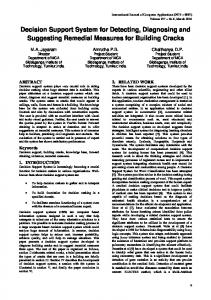
Research Article standards in ranking, thus helping a decision-maker to define their preferences by indicating an object that they like and an object that they do not like. The article presents the Preference Vector Method which is used for determining a decision-makers preferences depending on their needs. When solving their decision problems by means of the Preference Vector Method (PVM) a decisionmaker can express their preferences in various forms. Figure 1 shows various procedures of solving decision problems for different users’ preferences:  Variant A. A decision-maker specifies the name and the character of decision-making criteria that represent their preferences.  Variant B. A decision-maker specifies the name and the character of decision-making criteria as well as the preference vector values of one real object.  Variant C. A decision-maker specifies the name and the character of decision-making criteria as well as the preference vector value expressing the relevance of individual criteria.  Variant D. A decision-maker specifies the name of decision-making criteria and the values of motivating and demotivating preference vectors corresponding to real objects.  Variant D. A decision-maker specifies the name of decision-making criteria and the values of motivating and demotivating preference vectors corresponding to real objects.

PVM, Criteria X1 , X2 ………Xn character of criteria desirable (d), undesirable (nd), motivating (m),

demotivating (dm), neutral (n) A)

C)

B)

Objects

Just the criteria and the preference vector criteria

Criteria values of one real object

Name of object

DB

X1 MPV DMPV

X2

Xn

0.3 0.9 …… 0.5 0.2

D)

Values of object criteria

Objects

Explicit criteria values

Criteria values of two real objects

X1 X2 Xn 0.5 0.7 …… 0.6

Name of objects

DB

DB

0.4 …… 0.3 X1 X2 Xn MPV 0.3 0.9 …… 0.5

X1 X2 Xn MPV 0.6 0.7 …… 0.2 DMPV

0.1 0.5 …… 0.4

Figure 1: Chosen possible variants of the PVM designed to solve decision-making problems © Copyright 2014 | Centre for Info Bio Technology (CIBTech)

1481


Research Article STAGES OF THE PREFERENCE VECTOR METHOD For the majority of variants the research procedure of calculating PVM is performed in six main stages: selecting the criteria, defining the criteria character, changing the criteria character, normalising the criteria values, determining the preference vector and, finally, constructing the ranking. Stage I – Criteria selection The choice of criteria is related to a decision-maker’s preferences. The criteria are selected according to a decision-making situation. Many of such situations can be attributed with a fixed set of criteria which can

X

be applied in similar cases. Further in the paper the criteria are denoted with a capital letter i . The index denotes the criterion number. A criterion defines the objects’ attributes that can be expressed in

X

numbers. In the paper the objects will be denoted as j , where j is an object number. For example, for a given decision-maker the criteria that describe cars can be fuel consumption, engine power, etc. Such

xi criteria are expressed in values of

j

, i.e. by the value of the i-th criterion of the j-th object.

Stage II – Defining the criteria character The criteria that describe objects can be divided according to the values they are representing, such as:  desirable (d). The criteria where specific values are desired – not too big and not too small. For example: when buying a car a decision-makers expects a car of a specific size – too big or too small a car will not satisfy them.  undesirable (nd). The criteria where a specific value is not desired.  motivating (m). The criteria where high values are desired. For example, when choosing the terms for a bank deposit a decision-maker will be expecting maximum interest rates.  demotivating (dm). The criteria where low values are desired. For example, when buying something we want its price to be the lowest.  neutral (n). The criteria that are not relevant in the case of a given decision-making situation; their values should not influence the decision. In this stage we should attribute a certain character to each criterion. Stage III – Changing the criteria character When a decision-maker specifies the values of criteria they find desirable, they are treated as the weight of a preference vector (Figure 1, Variant C). In such a case we should change the character of the undesirable criteria into the desirable ones so that all the vectors that represent the objects can be directed compatibly to a motivating preference vector. Otherwise, a decision-maker would have to attribute demotivating criteria with a negative weight, while there is a principle often quoted in literature that weights must be positive. In such cases a change in the criteria character solves a decision-making problem thus influencing the study results and it is in accord with the logic of a decision-maker’s selection of weights. The next specific case may be a situation when a decision-maker specifies the values of criteria that are describing one real object (Figure 1, Variant B). Having decided on the criteria character and as a result of their normalising, some criteria may adopt negative values of their preference vector. Consequently, the motivating criteria are treated as demotivating, and vice versa – the demotivating ones are regarded as the motivating, which leads to the change of the preference vector’s direction. If we want to prevent it, we should reverse the values of this criterion. The reason why this problem occurs is associated with the applied normalisation method, because it does not happen in the case of methods that give only positive results. Thanks to the operations connected with the change of the criteria relevance, the direction of the motivating preference vector will agree with the directions of all the coordinate axes. © Copyright 2014 | Centre for Info Bio Technology (CIBTech)

1482


Research Article Stage IV – Normalising the criteria values In principle, the criteria describing the objects are not homogenous because they describe different parameters of these objects that are expressed in a variety of measures and have varying value scales. Consequently, data that are recorded in this way are incomparable. Therefore, it is necessary to reduce them to a form in which they can be compared. For that reason, the next stage of the PVM focuses on normalising the criteria, which results in the elimination of units of measure and brings the scale of values to a roughly identical level. The most common normalization method is standardization (Nermend, 2009):

xi 

xi  xi j

j

Si

,

(1)

where

xi j

xi j

– value of the i-th criterion of the j-th object, – value of the i-th criterion of the j-th object after standardization,

xi – mean value of the i-th criterion, S i – standard deviation from the i-th criterion. Stage V. Determining the preference vector The preference vector describes decision-maker’s preferences towards the analyzed objects. It can indicate what exactly a decision-maker is expecting – then we will call it a motivating preference vector. It will be denoted as MPVM and its elements as mpvmi. In the majority of the PVM variants there is just one preference vector of a motivating nature. In some PVM variants we can use a vector which specifies what a decision-maker does not want. Then it is called a demotivating vector and is referred to as DMPVM, while its elements are denoted as dmpvmi. How we interpret and determine the preference vectors depends on the PVM computation variant. This issue will be discussed in more detail in the further part of this paper which presents the PMV variants (Figure 1). In the computation process the preference vector is treated (in terms of the criteria character and their normalizing) in the same way as the other objects apart from Variant C. The change of the motivating vector’s criteria character should correspond to the changes regarding the objects, e.g. if we intend to change one criterion of the objects from motivating to demotivating, we have to make the same change in case of the preference vector. We should also normalise the motivating and the demotivating preference vector (or vectors) by means of the same normalizing parameters that have been used to normalize the criteria values. For example, the mpwmi vector can be normalized by means of standardization in a following manner:

mpvmi 

mpvmi  xi , Si

(2)

where

mpvmi mpvmi

– value of the i-th MPVM vector, – value of the i-th MPVM vector after normalization.


1483


Research Article Stage VI. Ranking In the ranking process each object is attributed with a numerical value describing its ranking position. For

X

this purpose we determine a component of the vector j which is representing an object along the preference vector MPVM  (Nermend, 2009; Nermend and Borawski, 2006): N

rj 

 x mpvm i 1 j N

i

i

 mpvm i 1

.

(3)

2

i

When the ranking is built on the basis of vectors selected as motivating and demotivating by a decisionmaker or computed automatically by the method, the above formula is (Nermend, 2006; Nermend, 2007): N

rj 





  x dmpvm mpvm  dmpvm i 1

i

i

i

N

 mpvm  dmpvm  i 1

where

i

j

,

(4)

2

i

i

dmpvmi – value of the i-th DMPVM vector after normalization, N – number of criteria.

The larger the value of

rj

, the higher the position of the j-th object in the ranking.

MATHEMATICAL DESCRIPTION OF THE VARIANTS PRESENTED IN FIGURE 1 (THE PREFERENCE VECTOR METHOD) Variant A. A decision-maker specifies their criteria and describes their character. In this variant we can only use criteria of a motivating or demotivating character. On the basis of these criteria we are building preference vectors (the motivating and the demotivating one). The formula for calculating the values of a motivating preference vector is (Nermend, 2009):

 xi  mpvmi  Q 3 x Q1i

for

m

for

dm

,

(5)

where m – the motivating criterion, dm – the demotivating criterion,

x

i Q1

– value of the first quartile for the i-th criterion,

xi

– value of the third quartile for the i-th criterion. The formula for calculating the values of a demotivating preference vector is (Error! Reference source not found.): Q3


1484


Research Article  xi dla m  . dmpvmi   Q1 x dla dm Q 3i

(6)

Variant B. A decision-maker specifies the criteria and the character of a motivating preference vector in a form of a real object. In this variant we can only apply the criteria of a motivating, demotivating and desirable character. The criteria creating a real object are introduced as the coordinates of a motivating preference vector. In this variant the manner in which the ranking is constructed is different – there are two rankings. One of them orders motivating and demotivating criteria. In the process of normalizing by means of standardization the ranking is constructed:

rj   xi mpvmi , v

iv j

(7)

n

where

 v – the set of indices of the X i criteria being motivating and demotivating, mpvmi

while

n

is a vector calculated:

  mpvmi   n  

mpvmi

for i  v

 mpvmk2

.

k  v

mpvmi

(8)

for i  v

The second ranking comprises the desirable values. Its calculation formula is: 2

  r j    xi  mpvmi  , i d  j d  where

v

– the set of indices of the

The ultimate value

rj

Xi

(9)

criteria being desirable.

is calculated:

rj N v  rj N d rj 

v

d

,

N v N d

(10)

where

Nv

– number of the motivating and demotivating criteria,

Nd

– number of the desirable criteria. Variant C. A decision-maker specifies the criteria value and describes its character which can be treated as the criteria weights. In this variant we can only use the criteria of a motivating or demotivating character and create only one preference vector:

mpvmi 

wi N

w i 1

,

(11)

i

where © Copyright 2014 | Centre for Info Bio Technology (CIBTech)

1485


Research Article

wi – weight for the i-th criterion. The values of weights neither change their sign nor are subject to normalizing. Calculations are possible only for motivating and demotivating values. Variant D. A decision-maker specifies the criteria of two preference vectors: the motivating and the demotivating one. The calculation proceeds automatically throughout stages I, II, IV, V and VI. The ranking based on motivating and demotivating vectors specified by a decision-maker is calculated by means of the formula (4). THE PREFERENCE VECTOR METHOD - CASE STUDIES Case study I In this paper the authors attempt to verify the method with the use of Eurostat data. They conduct a comparative analysis of the European Union countries in order to study their residential attractiveness for a decision-maker. The study is based on the Eurostat data of 2011 concerning those EU countries whose data were available in Eurostat. Seven criteria have been chosen: X1 -Expenditure on education as % of GDP public expenditure X2 -Financial aid to students X3 -Total R&D expenditure (GERD) by sectors of performance and type of R&D activity X4 -Business enterprise R&D expenditure (BERD) by economic activity and type of costs X5 -Unemployment rates of the population aged 25-64 by level of education X6 -Duration of working life X7 -Hospital beds The calculations were made according to Variant B. It was assumed that the decision-maker chose Germany as their motivating preference vector. They motivated their decision with the fact that Germany enjoyed a big national income and high standard of a social security system, which made it a good place to live. Such criteria as Expenditure on education as % of GDP public expenditure and Duration of working life were defined as desirable. In a citizen-friendly country expenses on education cannot be too small, because it would limit the access to education. On the other hand, they cannot be excessive since it is not in the country’s interest to provide education to everybody, but only to those who are actually willing to study hard. Mass high level education leads to its depreciation as well as to a high unemployment rate among graduates. As a result, money spent on education are wasted in terms of the country’s and its citizens’ interests because they could have been spent elsewhere. The citizens’ duration of working life is of similar nature. If it is too short, it means that their working conditions are bad and national health care system is inefficient. Neither can it be too long since the majority of citizens expect the retirement age to be early enough for them to be still able to enjoy it. The criterion titled Unemployment rates of the population aged 25-64 by level of education was defined as demotivating, while Financial aid to students, Total R&D expenditure (GERD) by sectors of performance and type of R&D activity, Business enterprise R&D expenditure (BERD) by economic activity and type of costs and Hospital beds as motivating. Table 1 shows the obtained values of

rj

for individual countries. In order to make the results easier to

r

read the values were divided into categories. The highest values of j were obtained by Germany which was a country of preference in this study, therefore the ranking was based on the similarity of all the objects to Germany. There were two types of approach to this similarity: in the case of desirable criteria all the remaining criteria were expected to reach the same level. As for the motivating and demotivating criteria, their values for Germany were regarded as an indicator of their significance. If some German

r

criteria values were bigger than for other objects, they automatically had a stronger effect on j . If they were smaller than the remaining criteria, their effect was weaker. Hence the method automatically prefers these criteria which distinguish a given object from the remaining ones. In the case of Germany the © Copyright 2014 | Centre for Info Bio Technology (CIBTech)

1486


Research Article Hospital beds criterion had the largest values among all the analized countries, thus having stronger effect on

rj

than the other criteria.

Table 1: Values of

rj

for individual countries

object

rj

class

object

rj

class

object

rj

class

Germany

0.714

1

Slovenia

-0.351

2

Ireland

-0.605

3

Austria

0.348

1

Lithuania

-0.371

2

Slovakia

-0.607

3

Finland

0.065

1

Estonia

-0.393

2

Romania

-0.795

3

Norway

0.058

1

Bulgaria

-0.46

3

Island

-0.877

4

France

-0.155

2

Latvia

-0.495

3

Italy

-0.908

4

Sweden

-0.16

2

Portugal

-0.549

3

Spain

-0.909

4

Czech

-0.238

2

Poland

-0.567

3

Cyprus

-0.918

4

Great

-0.3

2

Hungary

-0.584

3

Croatia

-0.936

4

-0.301

2

Britain Belgium

When analyzing the results, we can see that only four countries – Germany, Austria, Finland and Norway - have fallen into the first class. They are the best countries for the decision-maker to live in. Among them

r

it is Germany that has the highest values of j , which is a consequence of its being a country of preference. Yet, Variant B does not guarantee a country of preference to be always ranked first. Should other analyzed objects have higher values of motivating criteria and lower values of the demotivating ones, they can outscore the country of preference. It makes the ranking proper even when the country of preference is an object whose criteria values are weak. If there are objects in the ranking that are similar to the preferred one but having better parameters, there is no reason for them to be the object of preference themselves. A country that turned out to be the most similar to the preferred one was Austria. This is due to the fact that both countries are similar in terms of their social, geographical and historical background. The

r

following two countries, Finland and Norway, also fell into the first class, yet their j values were much lower and closer to the first top countries in the second class than to Germany and Austria. These countries have different background from Germany and Austria, which brings such discrepancies in the

rj

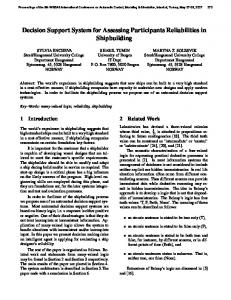
value. Although their quality of life is high as well, the importance of various aspects of life is perceived differently than in Germany, hence such vast discrepancies. When building a ranking based on an object of preference, we should always take into consideration the object’s attributes. In the presented example the positions in the ranking are determined by the object of preference. Some decision-makers may value the living standards in Germany, others may prefer to live in Norway or another country. The choice of Norway would change the ranking order but rather insignificantly. The countries with low criteria values would still remain at low positions although their ranking order might be different. Figure 2 shows a visualized form of the ranking. What we can see is a weak position of the Central European countries. Please remember, however, that they have just joined the European Union and that they had to abandon their centrally managed economies and adapt them to the free market demands. After the WWII their investments into technical infrastructure, science and industry were much lower © Copyright 2014 | Centre for Info Bio Technology (CIBTech)

1487


Research Article than in the west of Europe. This is why these countries are growing at a fast rate, with considerable support of the EU. When comparing the Central European EU states to other countries with similar

rj

r

values, we should take into account their j values in previous years in order to find out what the dynamics of their transformation is and to predict their development in the foreseeable future.

Class I Class II Class III Class IV

Figure 2: Classification of countries by their residential attractiveness Case study II A decision-maker is a researcher who would like to choose a country where investments in research and development are substantial, which would make their employment odds high. The data come from Eurostat. The authors made a comparative analysis of the European Union countries in order to study their residential attractiveness for the researcher. The analysis covered those EU countries whose 2011 data were available in the Eurostat database. Six criteria were chosen: X1 - Business enterprise R&D expenditure (BERD) by economic activity and type of costs X2 - Business enterprise R&D expenditure (BERD) by economic activity and source of funds X3 - Total R&D expenditure (GERD) by sectors of performance and type of R&D activity X4 - Total intramural R&D expenditure (GERD) by sectors of performance and source of funds X5 - Total intramural R&D expenditure (GERD) by sectors of performance X6 - Total R&D personnel and researchers by sectors of performance, as % of total labor force and total employment, and by sex Calculations were conducted in conformity with Variant A. All the criteria were defined as motivating. Table presents the values of

rj

for individual countries. Top positions were taken by countries with


1488


Research Article relatively small populations. In their study the authors used indicators normalized either by the number of residents or by the number of professionally active population. It means that proportionally to their population those countries’ expenditure on scientific research was the highest. Big countries, such as Germany which is a leader in many scientific fields, can spend more money on research, but per capita the numbers are not so impressive. Smaller countries, striving to remain competitive, must spend much more in proportion to the number of their inhabitants. In practice it means that the number of researchers in those countries in relation to their population can be larger than in big countries. Table 2: Values of

rj

for individual countries

object Finland Sweden Denmark

measure 1.953 1.883 1.822

class 1 1 1

Luxemburg Norway Austria Germany Island Belgium Holland France

1.576 1.468 1.318 1.234 1.034 0.981 0.893 0.886

1 1 1 2 2 2 2 2

object Ireland Slovenia Great Britain Italy Portugal Estonia Spain Czech Greece Hungary

measure 0.721 0.623 0.607

class 2 2 2

object Malta Lithuania Slovakia

measure 0.06 0.051 -0.012

class 3 3 3

0.326 0.318 0.315 0.314 0.251 0.076 0.075

3 3 3 3 3 3 3

Croatia Latvia Poland Cyprus Turkey Bulgaria Romania

-0.029 -0.05 -0.072 -0.072 -0.097 -0.138 -0.163

3 3 3 3 4 4 4

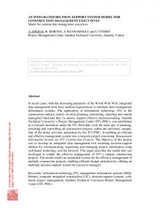
Figure 3 shows the classification of countries by their attractiveness for researchers. There is a clear division into what we used to call the West and East of Europe. The former take three top positions in the ranking leaving positions III –IV to the latter. What is more, the order is also determined by the time when individual states joined the European Union, which proves a strong impact of the EU on the way funds are allocated to support scientific research.


1489


Research Article

Class I Class II Class III Class IV

Figure 3: Ranking of countries by their attractiveness for researchers CONCLUSION The method presented in this article employs the preference vector to rank objects. It makes a decisionmaking process easier. A decision-maker can express their preferences by pointing out how important they find the individual criteria and what is their preferred or, if any, undesirable object. It is also possible to define preferences basing just on the character of criteria. However, the opportunity for a decisionmaker to specify their object of preference is important since it releases them from the necessity to understand the meaning of the criteria and their effect on the object. For example, a decision-maker may like fast sports cars, but they cannot quite understand how and which criteria influence a car performance. Therefore, specifying their object of preference is much easier for them. Two case studies were conducted by means of the proposed method. The studies presented in this article have confirmed the relevance of the method. The obtained results were logical and consistent with the authors’ expectations.

REFERENCES Borawski M. (2007). Rachunek wektorowy w przetwarzaniu obrazów, Wydawnictwo Uczelniane Politechniki Szczecińskiej Szczecin. Borawski M. (2012). Vector space of increments, Control and Cybernetics, 1. Duckstein L. and Gershon M. (1983). Multicriterion analysis of a vegetation management problem using ELECTRE II. Applied Mathematical Modelling 7 (4) 254– 261. Grabiński T. (1984). Wielowymiarowa analiza porównawcza w badaniach dynamiki zjawisk ekonomicznych, AE w Krakowie, seria specjalna: monografie, Kraków 61. Grolleau J. and Tergny J. (1971). Manuel de reference du programme ELECTRE II. Document de travail 24, SEMA-METRA International, Direction Scientiﬁque. Hellwig Z. (1968). Zastosowanie metody taksonomicznej do typologicznego podziału krajów ze względu na poziom ich rozwoju oraz zasoby i strukturę wykwalifikowanych kadr, Przegląd Statystyczny 4. © Copyright 2014 | Centre for Info Bio Technology (CIBTech)

1490


Research Article Karagiannidis A. and Moussiopoulos N. (1997). Application of ELECTRE III for the integrated management of municipal solid wastes in the greater Athens area. European Journal of Operational Research, 97 (3) 439–449. La Gauffre P. Haidar H. and Poinard D. (2007). A multicriteria decision support methodology for annual rehabilitation programs for water networks. Computer-Aided Civil and Infrastructure Engineering 22 478-488. Mousseau V. Figueira J. and Naux J. (2001). Unsing assignment examples to infer weights for ELECTRE TRI method: Some experimental results. European Journal of Operational Research, 130 (2) 263–275. Nermend K. (2006). A synthetic measure of sea environment pollution. Polish Journal of Environmental Studies 15 (4b) 127-130. Nermend K. (2007). Regions Grouping with Similarity Measure Based on Vector Calculus. Polish Journal of Environmental Studies 16 (5B) 132-136. Nermend K. (2008). Rachunek wektorowy w analizie rozwoju regionalnego, Wydawnictwo Naukowe Uniwersytetu Szczecińskiego, Szczecin. Nermend K. (2009). Vector Calculus in Regional Development Analysis, Series: Contributions to Economics, Springer ISBN: 978-3-7908-2178-9. Nermend K. and Borawski M. (2006). Using average-variance number system in calculation of a synthetic development measure. Polish Journal of Environmetal Studies 15 (4C) 127-130. Roy B., (1968). Classement et choix en presence de points de vue multiples (la methode ELECTRE). RIRO 8 57–75. Saaty T. (1980). The Analytical Hierarchy Process. McGraw-Hill, New York. Saaty T. and Thomas L. (2005). Theory and Applications of the Analytic Network Process: Decision Making with Benefits, Opportunities, Costs and Risks. RWS Publications, Pittsburgh, Pennsylvania. ISBN 1-888603-06-2. Scharlig A. and Pratiquer (1996). ELECTRE et PROMETHEE : Un Complementa Decider sur Plusieurs Criteres. Presses Polytechniques et Universitaires Romandes, Lausanne. Vallee D. and Zielniewicz P. (1994). ELECTRE III-IV, version 3.x, Aspects Methodologiques (tome 1), Guide dutilisation (tome 2). Document du LAMSADE 85 et 85bis, Universit´e Paris Dauphine


1491

modeling users' preferences in the decision support system - CIBTech

modeling users' preferences in the decision support system - CIBTech

Suggest Documents

Decision Support System in the Design, Production

Representing Users in a Travel Support System

Representing Users in a Travel Support System

Decision Support System for Detecting

Decision Support System for Assessing

Spatial Decision Support System (SDSS)

CLIPS based decision support system

decision support system to support decision processes with data ...

Decision Support system in modern education - wseas.us

Decision Support system in Physical Education - wseas

agent clinical decision support system

Indonesian Earthquake Decision Support System

Air Cargo Decision Support System

AN INTEGRATED DECISION-SUPPORT SYSTEM

Investigating Decision Support System (DSS)

Adaptive Decision Support System in Network Centric

multiple-criteria decision support system in highway

DECISION SUPPORT SYSTEM AND INTELLIGENT SYSTEM Book ...

Legitimate Grievances Preferences for Democracy, System Support ...

Legitimate Grievances Preferences for Democracy, System Support ...

The Ideal Engineering Decision Support System - CiteSeerX

The nitrogen decision support system: NitroGenius

Decision support system for determining the contact

Bail Decision Support System - THE IJES