Modeling Volume Change and Mechanical Properties ...

Modeling Volume Change and Mechanical Properties with Hydraulic Models Th. Baumgartl* and B. Ko¨ck ABSTRACT

Volume Change by Internal and External Stresses

Volume change of soils may be caused either by external (mechanical) or internal (hydraulic) stresses or a combination of both. A complete description of volume change must therefore include both mechanical and hydraulic stresses. By combining theories of mechanical and hydraulic stress states, a hydraulic function, which predicts the change of water volume as a function of the stress state parameter soil water suction (water retention curve), is adopted to model volume change. The utilization of such a continuous function also enables the derivation of soil mechanical parameters (e.g., preconsolidation stress, Youngs modulus) by determining mathematically the point of maximum curvature and inflection point. This information can then be used to calculate the preconsolidation stress according to the method of Casagrande. The presented calculation has considerable advantages compared with the graphic method of Casagrande or other methods. On the basis of stress–strain relationships of various textured and structured soils and soil substrates and various test procedures (oedometer test, triaxial test, shrinkage test), volume change is modeled using the described method. It is shown that modeling volume change by the van Genuchten equation using the software RETC is possible with high accuracy. Soil mechanical parameters are derived using the parameters of the van Genuchten equation. The comparison of results of this method with the Casagrande and a statistical method shows that these methods have deficiencies when the data sets have a high variability, the samples are not homogeneous, and when the stress–strain curve is flat. The accuracy of the mathematical method in contrast is very high and the calculated preconsolidation stress very reliable.

Processes of volume change in a porous system like soil can either occur in a two-phase system (solid–water or solid–air) or a three-phase system (solid–water–air). For reasons of simplification, it is generally assumed that air-filled pores are interconnected to the atmosphere and that the influence of pore air pressure buildup during volume changes can therefore be neglected. The stress state can be defined by two kinds of stresses within the soil. It is a result of external (mechanical) stresses and internal (hydraulic) stresses. Mechanical stresses are transmitted via the solid phase. Volume change occurs when maximum shear resistances between particles are exceeded. Hydraulic stresses or internal stresses are caused by the water phase in the pore system and influence the shearing resistances. When stresses are applied, they will be positive in a two-phase system (water-saturated soil), but may also be positive in the short term in a three-phase system (water-unsaturated soil), while compaction caused by external stresses will redistribute water into a pore system with a modified pore-size distribution. At the state of equilibrium of the water phase within the pore system (equivalent with the pore size distribution), hydraulic stresses will be generally negative and can be characterized by tensile stresses. Under unsaturated conditions, the change of internal stresses by wetting and drying will cause reduction or expansion of a soil volume. Depending on the intensity of the stress application, a deformation will be elastic or plastic. For a complete description of the stress state, both the external and internal stresses have to be combined as it is formulated in the Terzaghi equation (Terzaghi and Jelinek, 1954) for a two-phase system and in the extended form for a three-phase system, first described by Bishop and Blight (1963). This relationship is expressed as follows:

P

redicting volume change of soils under stress application is important when calculating the stability of soil substrates. This information is commonly used in engineering or agriculture to derive mechanical parameters (e.g., preconsolidation stress), which explain the stress history of a material. Preconsolidation stress, for example, shows which stresses a soil substrate has been exposed to in its history (mechanical, hydraulic) and up to which stress level it can be loaded without further unrecoverable volume change. Information about the kind of volume change is also important for the understanding of shrinkage behavior, crack and structure formation, as well as resistance to (shearing) stresses (Horn and Baumgartl, 2002). In the literature, various methods can be found which describe stress-dependent strain and the derivation of mechanical properties. However, many of these basic approaches lack in simplicity and uniqueness. A method is presented here which allows the description of volume change as a function of stresses based on hydraulic and mechanical stress state models and a well-defined derivation of mechanical properties using this theory.

␴⬘ ⫽ (␴ ⫺ ua) ⫹ ␹(ua ⫺ uw).

[1]

The stresses explained by the matric water potential of Eq. [1] represent the tensile stresses (Snyder and Miller, 1985), whereas the effective stresses are represented by the mechanical stress state. The ␹-factor of Eq. [1] accounts for the amount of water-filled pores which is, when defined as stress states, dependent on the matric water potential. Under saturated conditions, the parameter ␹ ⫽ 1 and Eq. [1] reduces to the general Terzaghi equation. It could be shown that this factor is explained within certain limits by the water retention curve (Baumgartl, 2002). The calculation of the tensile stresses is possible as long as the pore size distribution for each state of water potential is known (in fact, it is often assumed that the pore size distribution is constant). In principle, a calculation is possible even in soils with volume change (shrinkage or swelling, compaction), when the deformation behavior is known (Katou et al., 1987; O’Sullivan and Ball,

Th. Baumgartl, Inst. for Plant Nutrition and Soil Sci., Univ. of Kiel, Olshausenstrasse 40, 24118 Kiel, Germany; B. Ko¨ck, School of Mathematics, Univ. of Southampton, Southampton, SO17 1BJ, U.K. Received 19 Sept. 2002. *Corresponding author ([email protected]). Published in Soil Sci. Soc. Am. J. 68:57–65 (2004).  Soil Science Society of America 677 S. Segoe Rd., Madison, WI 53711 USA

57

58

SOIL SCI. SOC. AM. J., VOL. 68, JANUARY–FEBRUARY 2004

1993). Because volume change as a combination of compaction and shrinkage is very complex, deformation due to mechanical or hydraulic stresses are in the following viewed and modeled separately.

Adoption of the Stress–Strain Relationship with a Hydraulic Model In mechanical and agricultural engineering, the relationship of volume change with stress application is a common feature to describe the mechanical characteristics of soil substrates. With a semilogarithmic plot of normal stress vs. strain, a recompression curve at a lower stress range can be distinguished from a virgin compression curve at higher stresses (Casagrande, 1936; Terzaghi and Jelinek, 1954). Both curves are separated by the preconsolidation stress (Fig. 1). Likewise, volume change caused by increased internal stresses results in a relationship which behaves similarly (Fig. 1). At lower capillary stresses (i.e., less negative matric potentials), the shrinkage is smaller, whereas after exceeding a certain degree of dryness, the shrinkage rate increases with less negative matric water potentials. Within the range of small matric potentials, this relationship can be defined as the preshrinkage line. It is separated from the virgin shrinkage line by the preshrinkage stress (Baumgartl, 2002). The preshrinkage line at high matric water potentials is equivalent to the structural shrinkage of the wellknown shrinkage curve derived from the void ratiomoisture ratio relationship (Yong and Warkentin, 1975). The above considerations show that processes and the characteristic of volume change can be expressed similarly. Additionally, when both stresses occur, the mechanical and hydraulic stresses have to be coupled to define the complete stress state (Groenevelt and Bolt, 1972; Richards and Smettem, 1992; Richards et al., 2000). Fredlund and Rahardjo (1993) point out that several coefficients can be defined which formulate the volumetric deformation with hydraulic and mechanical

stress. For reasons of normalization in the following, pore volume is defined as the void ratio e (pore volume/ volume of solids) and water content as the moisture ratio ␽ (water volume/volume of solids). Figure 2 shows several possible scenarios. The application of mechanical stress on a water-saturated substrate (with ⌿ ⫽ 0 at drained conditions) may result in curve II (stress–strain relationship). The slope is defined by de/d␴. A steep slope at higher stresses (virgin compression curve) can be distinguished from a less steep slope at low mechanical stresses (preconsolidation curve). Taking the equivalent relation for hydraulic stress (⌿) vs. void ratio (e), the void ratio will decrease less with decreasing matric potential due to the emptying of pore space and hence reduced tensile stress. A possible relationship may be curve I in Fig. 2 and can be characterized as shrinkage-strain relationship. The slope at each point is defined by de/d⌿ and has low values at very low water potentials (preshrinkage curve) and very high water potentials (residual shrinkage curve). The curve in between these two ranges of water potential depict the virgin shrinkage curve. Referring the parameter moisture ratio ␽ to mechanical stress ␴ and assuming saturated conditions (with ⌿ ⫽ 0 at drained conditions), then this relationship is equivalent to curve II because ␽ ⫽ e. The slope is defined by d␽/d␴. When referring matric water potential ⌿ to moisture ratio ␽, the result may be curve III and describes the water retention curve (after Fredlund and Rahardjo, 1993). Similar considerations have been conducted by Toll (1995). He compared the shrinkage behavior of normally consolidated soil and overconsolidated samples with the moisture ratio and void ratio. He states that as long as a soil sample is saturated, the e–⌿ and ␽–⌿ relationships are identical. Once the sample starts to be desiccated, ␽ is reduced with further desaturation

Fig. 1. Stress–strain relationship as a consequence of compaction and shrinkage.

¨ CK: HYDRAULIC MODELS FOR VOLUME CHANGE BAUMGARTL & KO

following a virgin desiccation line with a steeper slope (curve III in Fig. 2). The slope of the e/⌿ relationship (curve I in Fig. 2) will remain constant as long as the shrinkage limit has not been reached. Beyond this point, the slope will reduce to zero. With the above given hypotheses, the similarity of volume reduction and change of water content due to hydraulic stress ⌿ can be referred to volume change due to mechanical stress ␴. Additionally, it has been described (Katou et al., 1987; Bruand and Cousin, 1995) that mechanical stress will first decrease the size of less stable coarse pores, which is comparable with draining coarse pores of a water-saturated soil first by increasing hydraulic stress. Furthermore, changes of the pore size distribution by mechanical stresses can be compared with the change of the pore size distribution by tensile stresses, although different in magnitude (see Eq. [1]). Combining these concepts of describing volume change by hydraulic and mechanical stresses provides a basis to model void ratio using an hydraulic model, which has been adapted to de/d␴ and de/d⌿ other than d␽/de. As a model, the van Genuchten-equation (van Genuchten, 1980) for determining of the water retention curve was chosen. The following expressions and parameters are used for different void ratio and moisture ratio relationships: (i) Moisture ratio ␽ vs. matrix potential ⌿ (water retention curve) ␽ ⫺ ␽r ⫽ [1 ⫹ (␣␽␺␺)n␽␺]⫺m␽␺ [2] ␽s ⫺ ␽ r (ii) Void ratio e vs. matric potential ⌿ (shrinkagestrain relationship) e ⫺ er ⫽ [1 ⫹ (␣e␺␺)ne␺]⫺me␺ [3] es ⫺ e r (iii) Void ratio e vs. total stress ␴ (stress–strain relationship)

e ⫺ er ⫽ [1 ⫹ (␣e␴␴)ne␴]⫺me␴ es ⫺ er

59 [4]

The parameters ␽s and es describe moisture ratio at water-saturated conditions and void ratio before stress application, respectively. The parameter ␽r (residual moisture ratio) is dependent on the texture of the material, but is often defined as ␽r ⫽ 0. The minimum (residual) void ratio er is dependent on the maximum packing density (i.e., minimum void ratio) of the material and will be generally around er ⫽ 0.27. The van Genuchten parameters ␣, n, and m have specific values (indicated by indices) depending on being related to void ratio or moisture ratio and mechanical stress ␴ or hydraulic stress ⌿. The advantage of this hypothesis is that it enables the definition of volume change by a simple and continuous function. Also, volume change due to external stresses can be expressed by the same model as volume change due to hydraulic stresses. In the case of shrinkage or swelling by internal stresses, the stress state parameter ⌿ and the functional relationship with moisture ratio and void ratio are the same.

Derivation of Soil Mechanical Properties Stress–strain relationships provide the basis to describe soil mechanical behavior. Such parameters can be, for example, preconsolidation stress or Youngs modulus. The preconsolidation stress is determined either graphically or statistically. The graphic determination after Casagrande (1936) defines this stress by use of the point of maximum curvature of the semilogarithmic stress– strain relationship. The preconsolidation stress is the point of intersection of two lines. The first line is the bisector line of the angle made by a horizontal and tangent line drawn at the point of maximum. The second

Fig. 2. Void ratio e and moisture ratio ␽ as a function of the dependent variable mechanical stress ␴ or hydraulic stress ⌿.

60

SOIL SCI. SOC. AM. J., VOL. 68, JANUARY–FEBRUARY 2004

line is the extended straight line of the virgin compression curve in direction to smaller stresses (Fig. 3). Although this method is commonly used, the determination of the point of maximum curvature and the decision of which range of stresses determine the virgin compression line are often subjective. Dias Junior and Pierce (1995) present a statistical procedure with which the difficulties of exact and objective determination of the Casagrande values can be excluded. They also compare this method with a number of different approaches. The method of Dias Junior and Pierce (1995) fits the recompression line and virgin compression line by a regression line starting with the smallest and highest applied stress, respectively. Stepby-step, the adjoined stresses for calculation of both regression lines are included and statistically compared. One combination of stresses, which determines the recompression line and the virgin compression line, will result in the greatest statistical difference of these two lines. Dias Junior and Pierce (1995) state a good agreement of this statistical method with graphic determinations. The preconsolidation stress is then defined as the point of intersection of these two lines. In practice, like the graphic method, this method has disadvantages when the number of observations is small and when the curvature of the log(stress)-strain relationship is small. Additionally, this method will only be an approximation dependent on the quality and number of data. With use of a continuous function, the soil mechanical parameters can be determined purely mathematically. On the basis of this hydraulic model of van Genuchten, the hydraulic/mechanical stress–strain relationship can be modeled with the above given boundary values. Volume change should always be defined by void ratio rather than relative strain. It simplifies calculations because residual void ratio can be defined by a constant value as explained above, whereas when using strain a specific bulk density has to be related to each soil and hence a specific minimum strain estimated. As the derived parameters of the van Genuchten curve respond very sensitively to the shape of the curve, it is quite important to model with a reliable residual pore volume (void ratio).

The mechanical parameter preconsolidation stress can be determined using the second and third derivation of this function. The virgin compression line is determined by the tangent through the inflection point (zeropoint of the 2nd derivation) of this function. The point of maximum curvature (1st zero-point of the 3rd derivation) is the starting point for the calculation of the bisector line of the angle made by a horizontal and a tangent line of the stress–strain relationship. When the zero-point of the 2nd and 3rd derivation is known, the point of intersection of the bisector and the extended straight line of the virgin compression curve can be calculated easily using a spread sheet. In the following, the derivation of the van Genuchten equation is described in detail. To simplify notations, the van Genuchten equation (see Eq. [2], [3], and [4]) is rewritten in the following uniform way: f(h) ⫽ (␪s ⫺ ␪r)[1 ⫹ (␣h)n]⫺m ⫹ ␪r,

[5]

with ␪s and ␪r being the water content at saturation and residual water content, respectively, and ␣, n, and m being the van Genuchten parameters. The variable h represents the matric water potential ⌿ or mechanical stress ␴. To take account for the logarithmic stress, f(h) is replaced by the following function: g(x) ⫽ f(10x) ⫽ (␪s ⫺ ␪r)[1 ⫹ (␣10x)n]⫺m ⫹ ␪r .

[6]

Furthermore, the notation k: ⫽ k(x): ⫽ ␣10 will be used. With use of k⬘(x) ⫽ k(x)ln(10) and the chain rule, the first derivative g⬘(x) of g(x) can be calculated as follows: x

g⬘(x) ⫽ (␪s ⫺ ␪r)(⫺m)(1 ⫹ kn)⫺m⫺1nkn⫺1k ln(10) ⫽ ckn(1 ⫹ kn)⫺m⫺1,

[7]

where c denotes the constant ⫺mn(␪s ⫺ ␪r) ln(10). With the addition of the product rule, the second derivative g″(x) and third derivative g⵮(x) of g(x) can be calculated as follows: g″(x ) ⫽ cnkn⫺1k ln(10)(1 ⫹ kn)⫺m⫺1 ⫹ ckn(⫺m ⫺ 1)(1 ⫹ kn)⫺m⫺2nkn⫺1k ln(10) ⫽ cn ln(10)kn(1 ⫹ kn)⫺m⫺2[(1 ⫹ kn) ⫺ (m ⫹ 1)kn] ⫽ c⬘(kn ⫺ mk2n)(1 ⫹ kn)⫺m⫺2,

[8]

where c⬘ denotes the constant cn ln(10). g⵮(x ) ⫽ c⬘[nkn⫺1k ln(10) ⫺ m2nk2n⫺1k ln(10)](1 ⫹ kn)⫺m⫺2 ⫹ c⬘(kn ⫺ mk2n)(⫺ m ⫺ 2)(1 ⫹ kn)⫺m⫺3nkn⫺1k ln(10) ⫽ c⬘n ln(10)kn(1 ⫹ kn)⫺m⫺3[(1 ⫺ 2mkn)(1 ⫹ kn) ⫺ (m ⫹ 2)(kn ⫺ mk2n)] ⫽ c⬘n ln(10)kn(1 ⫹ kn)⫺m⫺3[(1 ⫺ 2mkn ⫹ kn ⫺ 2mk2n ⫺ (m ⫹ 2)kn ⫹ m(m ⫹ 2)k2n] ⫽ c⬘n ln(10)kn(1 ⫹ kn)⫺m⫺3[1 ⫺ (3m ⫹ 1)kn ⫹ m2k2n] Fig. 3. Determination of the preconsolidation stress according to the method of Casagrande (1936).

[9] The zero

61

¨ CK: HYDRAULIC MODELS FOR VOLUME CHANGE BAUMGARTL & KO

hi ⫽ 10xi ⫽ 1/␣(1/m)1/n

[10]

of the factor 1 ⫺ mk of g″(x) is the inflection point of g(x). The zeros of g⵮(x) can be calculated by solving the discriminante of the quadratic polynomial n

1 ⫺ (3m ⫹ 1)Y ⫹ m2Y 2,

[11]

where Y :⫽ k ⫽ ␣ (10 ) ⫽ ␣ h . The first zero of this quadratic polynomial is n

n

Ymc ⫽

x n

n n

3m ⫹ 1 ⫺ √5m ⫹ 6m ⫹ 1 2m2

[12]

1 1/n 1 3m ⫹ 1 ⫺ √5m2 ⫹ 6m ⫹ 1 1/n Y mc ⫽ ␣ ␣ 2m2

冢

冣

Hydraulic parameters/relationships

Void ratio e Mechanical stress ␴ Distribution of Youngs modules E ⫽ ⌬␴/⌬e Stress–strain relationship e ⫽ f(␴) Stress–strain relationship e ⫽ f(␴)

moisture ratio ␽/water content ␪ water potential ⌿ pore size distribution ⌬␽/⌬⌿

Preconsolidation stress ␴p

water retention curve ␽ ⫽ f(⌿) shrinkage-strain relationship e ⫽ f(⌿) preshrinkage stress ␴s

x

g(xmc) ⫹ (1/2)g⬘(xmc)(xp ⫺ xmc) ⫽ g(xi) ⫹ g⬘(xi)(xp ⫺ xi)

[14] Hence, g(xi) ⫺ g(xmc) ⫹

1 g⬘(xmc)xmc ⫺ g⬘(xi)xi 2

1 g⬘(xmc) ⫺ g⬘(xi) 2

[15]

where the variables g(xi) and g⬘(xi) are given by g(xi) ⫽ f(hi) ⫽ (␪s ⫺ ␪r)[1 ⫹ (␣hi)n]⫺m ⫹ ␪r

It describes the elastic behavior of a material and is defined by E ⫽ ⌬␴/⌬ε.

[13]

The preconsolidation stress ␴p ⫽ 10 p can be calculated by equating the regression line through the inflection point with the bisecting regression line between the tangent at the point of maximum curvature and horizontal line (its slope is one half of the slope of the tangent regression line):

xp ⫽

Mechanical parameters/relationships

2

Thus, the maximum curvature of the function g is at hmc ⫽

Table 1. Comparison of mechanical and hydraulic parameters used.

[16]

and g⬘(xi) ⫽ ⫺mn(␪s ⫺ ␪r)ln(10)(␣hi)n[1 ⫹ (␣hi)n]⫺m⫺1, [17] respectively, and the variables g(xmc) and g⬘(xmc) are given analogously. Additional to preconsolidation stress, the Youngs modulus E is also an important mechanical parameter.

[18]

The strain can be replaced by the void ratio. According to this definition, the Youngs modulus describes the equivalent property mechanically as the pore size distribution (⌬␽/⌬⌿) hydrologically. Table 1 summarizes the hydraulic and mechanical parameters and relationships which are treated equivalently or are related to each other. MATERIALS AND METHODS Results of oedometer and triaxial tests from laboratory experiments and literature were used to model stress–strain relationships. The examples include stress–strain relationships caused by compaction as well as by shrinkage. In the case of compaction, a variety of differently textured and structured substrates with various bulk densities and utilization were investigated. Table 2 lists the main properties of the tested substrates. The oedometer tests were performed either with multiple replicates and a specific applied stress (oedometer test) or one sample was loaded continuously with increasing stresses (multistep test). The volume change with stress was modeled using the van Genuchten equation. The parameters ␣ and n of this model were calculated by RETC (U.S. Salinity Laboratory, 1999). The parameter m was fixed using m ⫽ 1 ⫺ 1/n. As the unit for mechanical stress is kilopascal, the ␣-value of the van Genuchten equation of the presented calculations has the unit 1/kPa.

Table 2. Investigated material. Substrate

Texture

Test

Soil

sandy loam

oedometer‡

Spoil

sandy loam

oedometer‡

Glacial till Palsa Clay-I Clay-II

loamy sand organic material loamy clay silty clay

oedometer† oedometer† oedometer‡ oedometer‡

Clay-III

silty clay (30%)

oedometer‡

Clay-IV-triax

clay (74%)

Kaolin K2

triaxial test (hydrostatic pressure) shrinkage

Kaolin K3

shrinkage

Remarks

Location

homogenised; natural bulk density; soil used for rehabilitation of a mine site homogenised; natural bulk density; spoil material used for rehabilitation of a mine site B-horizon, depth 40 cm; undisturbed undisturbed undisturbed; B-horizon of a Vertisol homogenized; maximum bulk density; base liner of a municipal landfill homogenized; maximum bulk density; base liner of a municipal landfill homogenized; low bulk density; base liner of a municipal landfill preconsolidation (28 kPa) and desiccation; data after Biarez et al. (1988) taken from Toll (1995) preconsolidation (55 kPa) and desiccation; data after Biarez et al. (1988) taken from Toll (1995)

Australia

† Indicates oedometer test with multiple increasing stress application of one sample (multistep-test). ‡ Indicates replicates applied with one specific load only.

Australia Germany Finland Germany Germany Germany Germany

62

SOIL SCI. SOC. AM. J., VOL. 68, JANUARY–FEBRUARY 2004

Table 3. Summary of results of modeling the stress–strain relationships with the van Genuchten equation and derivation of mechanical properties. Parameter Soil Spoil Glacial till Palsa Clay-I Clay-II Clay-III Clay-IV-triax Kaolin K2 Kaolin K3

e s†

er‡

␣§

n§

RMSE

NO¶

hmc#

hi††

␴p‡‡

0.705 0.941 0.481 5.364 0.980§§ 1.084 0.655 0.839 1.579 1.408

0.270§§ 0.270§§ 0.270§§ 0.270§§ 0.270§§ 0.270§§ 0.270§§ 0.270§§ 0.839 0.732

1/kPa 0.0314 0.0255 0.0074 0.1013 0.0212 0.0669 0.0191 0.0076 0.0094 0.0083

1.6419 1.9137 1.8116 1.3241 1.5397 1.3831 2.0921 1.2302 1.6318 1.5395

0.0118 0.0056 0.0020 0.0004 0.0236 0.0003 0.0239 0.0013 0.0003 0.0002

5 5 8 7 8 7 7 26 16 14

20 25 87 7 30 10 34 93 67 77

kPa 56 58 211 29 93 38 71 514 189 238

25 29 103 9 38 13 39 130 82 96

† es, modeled void ratio at stress ⫽ 0 kPa. ‡ er, minimum void ratio. § ␣ and n, van Genuchten parameters. ¶ NO, number of observations. # hmc, stress at maximum curvature. †† hi , stress at inflection point. ‡‡ ␴p, preconsolidation stress or preshrinkage stress. §§ fixed value during modeling.

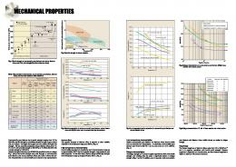
RESULTS AND DISCUSSION The principal results of the modeling procedure with RETC and the calculation of the preconsolidation stresses using the point of highest curvature and the inflection point of the van Genuchten equation are listed in Table 3. The results show that the volume change of all

Fig. 4. Data and model of the stress–strain relationship (compression) of the investigated substrates.

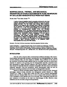
samples can be modeled with high accuracy as indicated by the RMSE value. Only the soil samples clay-I and clay-III have a higher deviation between data and fitted values. This is because of the relatively small number of replicates, but also because of the fact that each observation is represented by an individual sample. The heterogeneity between the replicates is high, particularly in structured samples, and the accuracy is therefore reduced. Regarding the oedometer tests with increasing stress on the same-sample (multistep) and the shrinkage test, the accuracy is very high. The results show that even when the heterogeneity of the data set is high, it is possible to find a well-fitted curve. Figures 4a, 4b, 4c, and 5 show graphically the modeled results. In Fig. 5, which shows the volume change of a shrinking soil, the calculated mechanical parameters (preshrinkage stresses) and the Youngs modules are included. The results of the tests depict very well the parameters structure and water potential, which influence soil mechanical properties and stability (Baumgartl and Horn, 1991). The combination of homogenized soil and low

Fig. 5. Data, model, and Youngs modulus of the stress–strain relationship (shrinkage) of the substrates Kaolin K2 and Kaolin K3 and preshrinkage stresses.

63

¨ CK: HYDRAULIC MODELS FOR VOLUME CHANGE BAUMGARTL & KO

water potentials at test conditions result in small preconsolidation stresses (soil, spoil, clay-I, clay-II, clay-III; Fig. 4a, 4c). The organic material of the substrate Palsa (Fig. 4b) with very high initial void ratio also presented a very low preconsolidation stress. The triaxial test was performed on homogenized material under isotropic conditions (Fig. 4c). This kind of compaction reduces the volume to a lesser extent. The steepness of the curve is lower and the calculated preconsolidation stress higher. The test on the structured glacial till (Fig. 4c) was performed at water conditions drier than field capacity. The sample originated from a site which was exposed to high stresses resulting from heavy agricultural machinery. The preconsolidation stress as a result of both the higher mechanical and hydraulic stresses, has to be classified as very high. The influence of both the mechanical compaction as well as the hydraulic impact of shrinkage can be observed in the samples Kaolin K2 and Kaolin K3 (Fig. 5; data taken from Toll, 1995, after Biarez et al., 1988). The sample Kaolin K2 was exposed to about 50% of the mechanical stress of Kaolin K3 (55 kPa). Both samples were then water saturated and dried. The preshrinkage stress which can be calculated from the shrinkage characteristic is higher than the mechanical preconsolidation stress. The shrinkage capacity of the kaolinitic substrate exceeds the mechanical compressing stresses when the material is dried and therefore increases the preconsolidation/shrinkage stress to higher values. Nevertheless, a memory effect can be recognized as the sample Kaolin K3 with higher mechanical preconsolidation stress, shows as well higher preshrinkage stresses after drying. The difference in the pretreatment is also identifiable in the elastic properties. The course of the Youngs modulus shows a higher width at lower water suctions for the substrate Kaolin K2 (Fig. 5). To value the mathematical method of deriving mechanical parameters from a functional relationship, the herewith calculated preconsolidation stresses are compared with the commonly used graphic method (Casagrande) and statistical method (Dias Junior and Pierce, 1995). The preconsolidation stress according to the Casagrande method was determined by a manual line of best fit. The statistical method consists of a four-parameter fit. As described earlier, two regression lines are calculated using an increasing number of measured data for the first regression line and a equivalently decreasing number of observed data for the second regression line. The regressions with the highest statistical difference were used to calculate the preconsolidation stress. The preconsolidation stress of the three methods are summarized in Table 4. The results of the methods differ partly to a great extent. The variation between the physical and mathematical method is higher with greater heterogeneity of the data set; that is, the less a true line could be drawn through the points (e.g., clay-I, clay-II). The statistical method has a high deviation when the slopes of the recompression line and the virgin compres-

Table 4. Comparison of preconsolidation stresses using different methods. Graphical Statistical Mathematical (Mohr-Coulomb) (four-parameter fit) (van Genuchten) Soil Spoil Glacial till Palsa Clay-I Clay-II Clay-III Clay-IV-triax Kaolin K2 Kaolin K3

20 18 80 18 68 32 22 145 105 85

kPa 21 17 73† 6 46† 71† 112† 49 35† 37†

25 29 103 9 38 13 39 130 82 96

† Not statistically significant from second best fit.

sion line are similar as a cause of either a small number of points (e.g., clay-II, clay-III) or a shallow stress–strain relationship in case of mechanical stress application (glacial till, clay-IV-triax) or reduced volume change in case of shrinkage (Kaolin K2, Kaolin K3). The comparison shows that the quality of the preconsolidation stresses of the graphic and the statistical method are very much dependent on the range of the applied stresses, which later define the recompression and virgin compression line. The accuracy also improves with greater homogeneity of the samples, that is, the more the slopes differ from each other. Regarding shallow stress–strain relationships with only little difference between the slopes of the recompression and the virgin compression line, the risk of small accuracy will always be high. The mathematical method allows a continual fit of the stress–strain relationship including the boundary conditions initial and residual void ratio and improves the accuracy of the derived preconsolidation stress (according to the Casagrande method). The shape of the stress–strain relationship modeled with the van Genuchten equation is based on the parameters ␣ and n. A sensitivity analysis shows that generally the preconsolidation stress is mainly influenced by the ␣-value of the van Genuchten equation. For n values ⬎ 1.6, the influence of n on the preconsolidation stress is negligible (Fig. 6). Only for stress–strain relationships with a small change in void ratio with increasing mechanical or hydraulic stress, that is, a small steepness of the van Genuchten equation, will n values have an influence on the value of the preconsolidation stress. As the shape of the curve has a sensitive influence on the calculated value of the preconsolidation stress, void ratio should be preferably used instead of, for example, an absolute or relative strain value. In the hydraulic use of the van Genuchten model, the ␣-value represents the air-entry value, which may be defined as the elastic property of the pore system in respect to emptying of water filled pores (Hillel, 1998). Hence, for high n values in very deformable substrates, the preconsolidation stress is equivalent to the air entry-value. The results of the modeling procedure show that it is possible to predict stress–strain relationships by a hy-

64

SOIL SCI. SOC. AM. J., VOL. 68, JANUARY–FEBRUARY 2004

APPENDIX List of Parameters ␴⬘ ␴ ⌿ ua uw ␹

Fig. 6. Influence of the van Genuchten parameters ␣ and n on the value of the preconsolidation stress (isobars in kPa; ␣ in 1/kPa).

draulic function (van Genuchten-equation) and to derive mechanical parameters like preconsolidation stress and Youngs modulus from derivatives of that equation.

CONCLUSION The combination of the theories which describe stress state functions of mechanical and hydraulic stresses and the utilization of a model, which describes the behavior of volume change due to either mechanical or hydraulic stresses, bears great advantages when modeling volume change. The application of a continuous function enables the inclusion of soil mechanical information in respect to stress–strain behavior into soil compaction models and to model stresses and stress distribution in soils. In regard to shrinkage, the stress state parameter soil water suction controls volume change. Shrinkagerelated parameters like preshrinkage stress can also be easily derived from a continuous function as soil mechanical parameters such as preconsolidation stress. In comparison with existing methods, the mathematical method has the advantage to easily derive soil characteristics from this continuous function. Furthermore, the modeling of the stress–strain relationship is based on the boundary conditions initial and final void ratio and increases the accuracy of the result in case of data sets with high variability. Furthermore, the utilization of the same function for mechanical and hydraulic processes simplifies the coupling of both these processes and enables one to relate the stress state parameters mechanical stress ␴ to hydraulic stress ⌿. This is of great advantage when the total stress state of soils has to be defined.

␪ ␪s ␪r ␽ ␽r ␽s e er es ␣ n m h E ε ␴p ␴s

effective stress total stress water potential pore air pressure pore water pressure ⫽ water suction [ ⫽ ⫺⌿ (matric water potential)] parameter related to the degree of saturation of the soil (0 ⱕ ␹ ⱕ 1) water content water content at saturation residual water content moisture ratio residual moisture ratio moisture ratio at saturation void ratio residual (minimum) void ratio (e ⫽ 0.27) maximum void ratio van Genuchten parameter (subscripts relate to the dependent variables e, ␽ and ␴, ⌿) van Genuchten parameter (subscripts relate to the dependent variables e, ␽ and ␴, ⌿) van Genuchten parameter (subscripts relate to the dependent variables e, ␽ and ␴, ⌿) variable representing ␴ or ⌿ Youngs modulus strain preconsolidation stress preshrinkage stress REFERENCES

Baumgartl, T. 2002. Prediction of tensile stresses and volume change with hydraulic models. p. 550. In M. Pagliai and R. Jones (ed.) Sustainable land management—Environmental protection: A soil physical approach. Catena Verlag, Reiskirchen, Germany. Baumgartl, T., and R. Horn. 1991. Effect of aggregate stability on soil compaction. Soil Tillage 19:203–213. Biarez, J., J.M. Fleureau, M.I. Zerhouni, and B.D. Soepandji. 1988. Variations de volume des sols argileaux lors de cycles de drainagehumidification. Rev. Fr. Geotechnique 41:63–71. Bishop, A.W., and G.E. Blight. 1963. Some aspects of effective stress in saturated and partly saturated soils. Geotechnique 13:177–197. Bruand, A., and I. Cousin. 1995. Variation of textural porosity of a clay-loam soil during compaction. Eur. J. Soil Sci. 46:377–385. Casagrande, A. 1936. The determination of pre-consolidation load and its practical significance. p. 60–64. In Int. Soil Mech. Found. Eng. Harvard University, Cambridge, MA. Dias Junior, M.S., and F.J. Pierce. 1995. A simple procedure for estimating preconsolidation pressure from soil compression curves. Soil Technol. 8:139–151. Fredlund, D.G., and H. Rahardjo. 1993. Soil mechanics for unsaturated soils. A. Wiley, New York. Groenevelt, P.H., and G.H. Bolt. 1972. Water retention in soils. Soil Sci. 113:238–245. Hillel, D. 1998. Environmental soil physics. Academic Press, San Diego, CA. Horn, R., and T. Baumgartl. 2002. Dynamic properties of soils. p. 389.

¨ CK: HYDRAULIC MODELS FOR VOLUME CHANGE BAUMGARTL & KO

In A.W. Warrick (ed.) Soil physics companion. CRC Press, Boca Raton, FL. Katou, H., K. Miyaji, and T. Kubota. 1987. Susceptibility of soils to compression as evaluated from the changes in the soil water characteristic curves. Soil Sci. Plant Nutr. (Tokyo) 33:539–554. O’Sullivan, M.F., and B.C. Ball. 1993. The shape of the water release characteristic as affected by tillage, compaction and soil type. Soil Tillage Res. 25:339–349. Richards, B.G., T. Baumgartl, and R. Horn. 2000. Modeling coupled processes in structured unsaturated soils—Theory and examples. p. 175–190. In R. Horn et al. (ed.) Subsoil compaction: Distribution, processes, consequences. 32nd ed. Catena Verlag, Reiskirchen, Germany. Richards, B.G., and K.R.J. Smettem. 1992. Modeling water flow in two- and three-dimensional applications. I. General theory for nonswelling and swelling soils. Trans. ASAE 35:1497–1504.

65

Snyder, V.A., and R.D. Miller. 1985. Tensile strength of unsaturated soils. Soil Sci. Soc. Am. J. 49:58–65. Terzaghi, K., and P. Jelinek. 1954. Theoretische Bodenmechanik. Springer Verlag, Heidelberg, Germany. Toll, D.G. 1995. A conceptual model for the drying and wetting of soil. p. 805–810. In E. E. Alonso and P. Delage (ed.) First Int. Conf. on Unsaturated Soil, Paris. 6–8 Sept. 1995. Balkema, Rotterdam, the Netherlands. U.S. Salinity Laboratory. 1999. Code for quantifying the hydraulic functions of unsaturated soils. Release 6.0. U.S. Salinity Lab., USDA, ARS, Riverside, CA. van Genuchten, M.T. 1980. A closed-form equation for predicting the hydraulic conductivity of unsaturated soils. Soil Sci. Soc. Am. J. 44:892–898. Yong, R.N., and B.P. Warkentin. 1975. Soil properties and behaviour. Elsevier, Amsterdam.