Eleventh International IBPSA Conference Glasgow, Scotland July 27-30, 2009
MODELLING AN EXISTING BUILDING IN DESIGNBUILDER/ENERGYPLUS: CUSTOM VERSUS DEFAULT INPUTS Holly A. Wasilowski and Christoph F. Reinhart Harvard University, Graduate School of Design Cambridge, MA, USA
[email protected],
[email protected]
ABSTRACT This paper describes an effort to build and partially validate an energy model of an existing educational building located in Cambridge, MA, USA. This work was carried out as part of a research seminar for graduate architecture/design students and included four related tasks: Modelling the building’s geometry and thermal properties in DesignBuilder/EnergyPlus, generating a site-specific weather file based on nearsite measured data, assessing internal load schedules based on a detailed building survey, and collecting monthly metered data for heating lighting and cooling over a whole year. The purpose of the seminar was (a) to evaluate how effectively design students can use a state-of-the-art graphical user interface (GUI) such as DesignBuilder and (b) to quantify the value of using customized weather data and internal load schedules as opposed to default GUI inputs. The authors found that the students quickly learned how to navigate the DesignBuilder GUI but were frequently confused by the model data hierarchy/inheritance and frustrated that customized schedules cannot be assigned more efficiently. The benefit of using customized weather data as opposed to a local TMY3 file turned out to be small whereas using customized as opposed to default internal load schedules reduced the relative error of predicted versus metered annual electricity use from 18% to 0.2%. Keywords: measurement & verification, energy simulation, occupant behaviour, benchmarking
INTRODUCTION Across the North American building design industry, there is a growing interest in computer-based building energy simulations. One of the drivers for this change is a rising awareness of sustainable design practices among building owners and policy makers and – as a direct result – an exponentially rising number of so-called ‘green’ new construction and renovation projects. In North America, the US Green Building Council’s LEED (Leadership in Energy and Environmental Design) rating system (USGBC 2009) has established itself as a de-facto industry standard to demonstrate the ‘greenness’ of a building. Most projects rated under LEED require an
energy model to establish the number of energyefficiency credits for which the project is eligible under LEED. One outcome of the above-described rising demand for building performance simulation is an acute shortage of qualified consulting engineers who can provide their services to design teams. Until now, energy modelling has generally been performed by mechanical engineers or specialized consultants. This practice has lead to the dilemma that integrated design practice, i.e. early involvement of the energy consultants in the design process, leads to increased up-front costs. In this climate, design teams might reconsider the notion of ‘who’ should actually carry out an energy simulation. While much of the more advanced modelling tasks involving complex HVAC systems and advanced system integration are likely to stay in the domain of engineer and energy consultants (Augenbroe, 2002), architectural firms might actual want to start building up at least some energy modeling capabilities in-house. The most recent generation of commercial, high-end graphical user interface seems to cater to the needs of architectural firms with the developers suggesting that these tools have become so intuitive that they can be used by "everyone, even architects”. The potential benefits for architectural firms to add energy simulations to their portfolio are shorter communication paths and more effective design feedback loops leading to shorter design times. The disadvantages are equally clear as this could turn into one more task that the architect must take on without necessarily increasing project budgets. These potential advantages and shortcomings notwithstanding, an initial question worth investigating is whether the current generation of energy modelling software can actually be easily picked up by architectural students. Schmid recently reported his experiences of teaching energy simulation to architectural students in Brazil (Schmid, 2008). He found that students could ultimately learn how to use energy modelling software, but they expressed difficulty with the “user-friendliness” of the interface. One of the limitations of the Schmid study was that the students used a simulation model written by one of the study authors. This model had a basic GUI but nothing comparable to some of the advanced current
- 1252 -
commercial tools such as Sketchup/OpenStudio (Google, 2009 and NREL, 2009), Ecotect (Autodesk, 2009) and DesignBuilder (DesignBuilder, 2009). All three tools allow the user to build relatively complex building geometries and to export them into EnergyPlus for an energy simulation (US-DOE, 2009). For this study, the authors used the DesignBuilder software since it also comes with extensive data templates for a variety of building simulation inputs such as typical envelope construction assemblies, lighting systems, and occupancy schedules. These templates can be especially enticing to beginners who may not have a sense for when more accurate inputs specific to their building may be desirable. This invites the question, "in which situations are these templates an acceptable shortcut, and in which situations is it worth the effort to generate custom inputs?" This paper investigates two questions: How successful can a group of architectural students learn how to build an energy model of a complex commercial building over the course of a 13-week term and how much accuracy can be gained by using customized weather data and internal load schedules as opposed to default DesignBuilder inputs. These two questions were addressed as part of a research seminar on ‘Building Performance Simulation – Energy’ that was offered during the Fall 2008 term at Harvard University’s Graduate School of Design (GSD). The case study building was the GSD’s own building, Gund Hall, located in Cambridge, MA, USA.
METHODOLOGY Overview As stated above, the initial goal of the research seminar was to build and evaluate a model of Gund Hall using the DesignBuilder interface for the EnergyPlus simulation engine. Eleven graduate students with various professional backgrounds, including several practicing architects but no mechanical engineers, worked on this task. Gund Hall is a 16,350 gross m2 iconic modernist building built in 1972 that exhibits a number of features that make it an interesting modelling object. Not only does Gund Hall have the expected academic functions involving classrooms and offices, but also a library, workshops, a small cafeteria, and a large 24-hour studio space with seemingly erratic occupant schedules. The studio consists of a large open space with multiple levels of balconies and a stepped, ziggurat-like roof. The building has over 100 separate roof surfaces and its envelope is characterized by large areas of glazing and exposed concrete (see Figures 1 and 2). In addition, Gund Hall is a multi-faceted building serving a multitude of programs which vary throughout the year. However, given that the building is connected to the campus’s district steam and chilled water system, the
building does not include an on-site heating and cooling plant, somewhat simplifying the HVAC modelling and reducing the impact of part-load performance curves. The students divided into four groups: a weather group, modelling group, HVAC & metered energy group, and survey group. Each group spent approximately six weeks on their individual tasks, and at the end, combined the information into one model of Gund Hall. The sections below describe this work in more detail.
Figure 1 Photo of Gund Hall
Figure 2 DesignBuilder Model of Gund Hall Weather Group Gund Hall is located in Cambridge, Massachusetts, USA, which is part of the Boston Metropolitan Area. A TMY3 weather file for Boston-Logan Airport is available from the U.S. Department of Energy EnergyPlus climate file database (US-DOE 2009). TMY3 data sets are derived from the 1991-2005 National Solar Radiation Data Base (NSRDB) archives, i.e. they represent typical meteorological conditions over several years. In order to compare energy model predictions to metered energy use for Gund Hall the Weather Group compiled two custom EnergyPlus Weather (EPW) files. The first file (EPW1) included data from November 1, 2007 to October 31, 2008. The data necessary was not readily available from a single source; therefore, data was acquired from three Boston & Cambridge area weather stations, and then aggregated into an EPW format. Dry bulb temperature, dew point temperature, relative humidity, atmospheric station pressure, wind speed, and wind direction were acquired from data collected on the roof of the Green Building on the Massachusetts Institute of Technology’s (MIT’s) Cambridge campus.1 Radiation data was acquired from the University of Massachusetts-Boston’s Center for Coastal 1
Green Building location: 2.6 km from Gund Hall. Weather station hardware: Davis Vantage Pro 2 Software: VWS V12.08
- 1253 -
Environmental Sensing Networks (UMass-Boston).2 All of the other data for EPW1 was drawn from the default Boston-Logan TMY3 file. For some individual hours or days, MIT or UMass-Boston data was unavailable; therefore, data was inserted from the Boston-Logan TMY3 file. This likely causes some inconsistencies and abrupt jumps in the weather data. The second EPW file, “EPW2,” included weather data collected on top of Gund Hall from October 29 until December 4, 2008; the balance of the weather file was the Boston – Logan TMY3 file. The Gund Hall data was collected using a temporary HOBO3 weather station, shown in Figure 3. The weather station collected wind speed, wind gust speed, wind direction, dry bulb temperature, relative humidity, dew point, and solar radiation in hourly time steps.
Figure 3 Gund Hall Weather Station Geometry Group The responsibility of the geometry group was to model Gund Hall in DesignBuilder using drawings from multiple renovations (see e.g. Figure 4). The resulting DesignBuilder model contains over 100 different zones, 8 different exterior wall types, and 5 different window types. Envelope properties were taken from an earlier Gund Hall analysis report written by Transsolar Inc. (Voit et al., 2007). The overall mean U-factor for Gund Hall is 2.45 W/m2K, a high value for this climate by today’s standards, due to large expanses of single-paned glazing and uninsulated fibreglass roof panels (Voit et al., 2007). HVAC & Metered Energy Group The HVAC and Metered Energy Group collected information about Gund Hall’s HVAC system design and operation for input into the model. They also gathered utility records for use in evaluating the model results. Electricity is provided by Cambridge Electrical Distribution. Building heat and domestic hot water derives from high-pressure steam from dual-fuel boilers at a central plant. Similarly, cooling for air 2
UMass-Boston location: 9.4 km from Gund Hall. Weather station hardware: Davis Vantage Pro Plus. Software: unavailable. 3 HOBO weather station, Onset Computer Corporation, Bourne, MA. www.onsetcomp.com Includes: weather station starter kit, HOBO software, solar radiation sensor, light sensor level, and tripod kit.
conditioning comes from chilled water, produced by a central plant. All energy consumption is metered at the building, rather than plant level. The Gund Hall facilities manager provided an overview of the Gund Hall HVAC system and the operation schedules for the nine Air Handling Units (AHUs). Due to current limitations in the DesignBuilder GUI, purchased steam and purchased chilled water were not available options for heating and cooling and instead were modelled as fan coil units. In addition to the central AHUs Gund Hall utilizes both radiant heat and VAV systems with steam reheats. These systems were excluded from the model, a known shortcoming that will be discussed later. The only spaces in Gund with operable windows are some of the offices. In these spaces, natural ventilation was turned on in the model and set to be automatically controlled by DesignBuilder based on occupancy schedule and indoor/outdoor temperature differences. Annually, Gund Hall uses 160 kWh/m2 for heating, 180 kWh/m2 for cooling, and 146 kWh/m2 for electricity for a total of 486 kWh/m2. The national average for a university building is 378 kWh/m2 and 361 kWh/m2 for a regional office building (regional university data is unavailable.) www.eia.doe.gov/emeu/cbecs/cbecs2003/detailed_ta bles_2003/detailed_tables_2003.html (CBECS, 2003). Therefore, Gund Hall uses approximately 32% more energy than comparable buildings, presumably due in part to its poor envelope performance.
Figure 4 First floor of model with imported floor plan below. Survey Group The objective of the Survey Group was to collect information on Gund Hall’s internal load schedules from building occupants, plug-loads and electric lighting as well as window shade operation for input into the Design Builder model. The information was collected during October/November 2008 and estimated for the rest of the year. The Survey Group separated the spaces of Gund Hall into twenty-three
- 1254 -
categories, each category having similar use characteristics. The Survey Group conducted twenty walk-though observations of Gund Hall. In addition to these observations, an online questionnaire regarding occupant schedules and appliance usage was sent to building occupants. Approximately 22% of 600 occupants responded to the questionnaire. The selfreported occupancy was higher in each time-slot than the observed occupancy by an average of approximately 20%. Since both methods of data collection have their own limitations, the average occupancy schedule derived from the two methods was used for the DesignBuilder model. The survey data was collected over a four-week period during the normal academic session. Therefore, to account for the summer term and various holiday breaks, the Survey Group created schedules for 5 additional calendar periods based on estimates provided by the facilities manager. For example, during spring break, the occupancy of the studios was multiplied by 0.4 for each time slot. The classroom occupancy schedules were created by manually linking classroom-booking appointments from October to November 2008 with a class enrolment list. A total of 19 different occupancy schedules were generated for the model. The Survey Group also calculated plug-load densities for each space and seven different plug-load schedules. As part of this effort, the group metered ten commonly used pieces of equipment in Gund Hall to determine their actual wattage using a wattmeter4. Since equipment use is directly connected to occupancy, the researchers linked the equipment schedule with the occupancy schedule. Equipment was divided into those appliances which would be active as a percentage of the students’ presence in the studio (i.e. lamps, coffee machines etc.), and those appliances which would have a constant wattage regardless (i.e. refrigerators). For the “active consumption”, the quantity of each type of appliance was converted into a ratio per student. The wattage per student was then multiplied by the occupancy fraction for each time slot and added to the base wattage consumption. Due to the high wattage used by most of the electronic equipment in the wood shop, the Survey Group could not monitor their use over time with the available watt meters. In order to sidestep this problem the band saw was metered over a week, and its usage pattern identified. The same usage pattern was then assumed for the rest of the wood shop equipment.
4
Watt meters used: watts up? Pro ES by Electronic Education Devices, www.wattsupmeters.com and Kill A Watt EZ P4460 by P3 International Corporation, www.p3international.com.
For equipment in the cafeteria kitchen, peak loads were assessed based on equipment labels or internet product searches. The average operating power for that equipment was then estimated based on typical usage information provided by the cafeteria manager. For equipment that cycles on and off such as refrigerators, annual energy consumption estimates were obtained from the Energy Star Restaurant Guide (U.S. EPA, 2007). Since the plug-loads in the offices seemed fairly typical, the equipment power density, 5.4 W/m2, suggested by professional energy consultants, Simpson Gumpertz & Heger was used (Waite, 2008). The Survey Group also calculated lighting power densities for each of the 23 space categories based on observation of each space, a list of lamp types provided by the facilities manager, and wattage information from the internet. The group then created four unique lighting schedules, based on information from the facility’s manager, for spaces in which the lighting operation is independent from the occupancy schedules. In addition, four different window shade schedules were created based on questionnaire responses, walk-though observations, and an interview with the facility manager. Simulations Finally, the work of the four groups was combined into a DesignBuilder model. One set of three simulations was run using each of the weather files: the Boston – Logan Airport TMY3 file, “EPW1” the composite UMass/MIT file, and “EPW2” the BostonLogan TMY3 file with one month of Gund Hall weather station data inserted. In another set of simulations, the natural ventilation and window shading were turned-off, one at a time, to isolate the impact of these features on the building’s energy consumption. To investigate the energy impact of occupant behaviour and the importance of surveying existing conditions, another series of simulations was run. This time several of the custom inputs were replaced with default inputs from the DesignBuilder database. First, the custom occupant densities and occupancy schedules were replaced with default densities and schedules. For each space, the most appropriate DesignBuilder template was chosen. For example, for the studio space, the DesignBuilder “University Open Office Occupancy” was used. The cafe kitchen became “University Food Prep Occupancy” and so on. Second, starting with the revised model described above, the custom plug-load densities and schedules were replaced with default DesignBuilder values in the same manner. Third, starting with this model, the custom lighting schedules were similarly replaced. In this model, the lighting densities were also changed to default values by first setting each space to the IECC-2000 template standard of 3.4 W/m2 per 100 lux and then changing the target illuminance in
- 1255 -
each space per the DesignBuilder templates. The default target illuminances ranged from 50-500 lux depending on the space type. Finally, the custom heating & cooling schedules were replaced with default values for “University Open Office.”
RESULTS Weather Files As one might expect, the data in all three weather files is similar except for wind speed, which is a very site-specific phenomenon. Comparing EPW1 (the MIT/UMass-Boston file) and the default file for the year reveals a daily mean difference in outside drybulb temperature of 0.12 oC and 2.85 m/s in wind speed. Comparing EPW2 (the Gund file) and the default file, for the 37 days for which Gund Hall data was recorded, reveals a daily mean difference in outside dry-bulb temperature of 0.61 oC and 4.73 m/s in wind speed. The heating load results of annual simulations using EPW 1 and EPW 2 are shown in Figure 5 along with actual measured heating consumption. The November data in EPW 2 was obtained on-site. The rest of EPW2 is an amalgamation of multiple years meant to represent a “typical year.” Therefore, one would expect EPW 1 to produce results that are more accurate in these months. However, one can see that, on a monthly or annual scale, both weather files produce similar accuracy. The same is true for cooling consumption. The remainder of the simulations discussed below used the EPW 1 weather file.
of the model’s glazing. The annual heating load increases by 0.3% and the annual cooling load decreases by 0.14% with the addition of shades. Electricity Figure 6 compares measured monthly electricity use for Gund Hall from August 2007 through July 2008 to simulations using different combinations of custom and default internal loads. As one would expect, the fully customized loads followed the metered electricity use more closely than simulations based on default assumptions. For the fully customized loads the mean bias error (MBE) and root mean square errors (RMSE) were 0.2% and 23% respectively compared to -17% and 64% for the default loads. In order to better illustrate the significance of the different internal load sources, the dotted line in Figure 6 shows simulation results using default occupancy and equipment but customized electric lighting loads. For this case, the results fell about halfway between the fully customized and alldefault results, highlighting the significance of modelling internal loads for electric lighting adequately. Since the electric loads do not include heating and cooling, changing their schedules had no effect on the electric loads.
Figure 6: Electricity - Measured vs. Simulations
Figure 5: Heating Load Comparing Weather Files Natural Ventilation & Shading The researchers ran simulations with and without both natural ventilation and window shading in the model. The addition of natural ventilation caused a 7.3% increase in annual heating load, and a 2.6% decrease in annual cooling load. The significant increase in heating load is surprising and warrants further investigation into the DesignBuilder definition of the natural ventilation control set points chosen. The window shading had little impact on the heating and cooling loads, which is not surprising given that the shades are internal and present on less than half
Heating and Cooling The monthly metered and simulated heating and cooling loads are shown in Figures 7 and 8. The students found abnormalities in the metered chilled water data from 2007/2008, so data from the previous school-year are shown here. From these graphs, one can see that the use of custom versus default settings, including HVAC operating schedules, made some difference in the simulation results, but the impact (as a percentage of total load) is not as dramatic as with electricity.
DISCUSSION Energy Simulations for Architects Following the experience of a semester long-course on building energy simulation, several individual modelling exercises and the group project of modelling Gund Hall, the students were asked how comfortable they now felt with their modelling skills and whether they would use the software again. As novice energy modellers and non-engineers, they
- 1256 -
seemed to be reasonably satisfied with the simulation results from the course project and there was a general expectation that with minor tweaking of the settings, the simulation results could be brought into even better alignment with the measured data. Most students found that the exercise of modelling Gund Hall helped them understand the software better but at the same time they felt more comfortable using the software for smaller projects, where there is less room for modelling mistakes, and earlier in the design process, when more basic decisions regarding programming and massing can be made based on the software. DesignBuilder/EnergyPlus was chosen for this course because, in comparison to most other building simulation software, DesignBuilder is a state-of-theart GUI. However, it still did not meet the expectations of architecture students accustomed to using sophisticated CAD and 3D modelling tools. In particular, in DesignBuilder, the ability to select and organize model objects seemed limiting, and the system of templates and attribute inheritance seemed both inflexible and unintuitive compared to other software for architects. Conversely, the students needed to learn to abstract their models better. The students approached the geometries, schedules, and construction types with a minute level of detail much more appropriate for an architectural model than a building simulation. Nevertheless, in a survey, 10 out of 11 students said they would definitely recommend using DesignBuilder/EnergyPlus for comparing architectural design decisions. Known and Suspected Shortcomings While simulated and measured energy loads were reasonably close for the Gund Hall model, the authors do not rule out that hidden “lucky” mistakes may be cancelling out each other. Some of the know shortcomings of the model are: • The building’s HVAC system was simplified, therefore, the VAV system with steam reheats was not modelled, meaning simultaneous heating and cooling would be underestimated. • It is suspected that the building systems cannot actually meet the peak cooling loads. Therefore, the modelled cooling system, with its unlimited capacity, exceeds the utility load in July. • In addition, manual heating setbacks during the extended holiday and exam periods in late December and January were likely underestimated by the students in the model. Finally, the chilled water meter was suspected of malfunctioning and was replaced a few weeks prior to this writing. Therefore, the authors are unsure of the accuracy of the measured data shown in Fig. 8.
Figure 7: Heating – Measured vs. Simulations
Figure 8: Cooling – Measured vs. Simulation Weather Files Given the significant influence of weather conditions on building performance, it is essential to use reliable climate data for energy modelling. Given that each of the three weather files tested produced similarly accurate simulation results, any of the three would have been acceptable for this project. This is not surprising given that all three files were collected within a relatively small radius of several kilometres. The different files had some significant discrepancies in local wind conditions, but since the energy use of Gund Hall is not very susceptible to wind, these differences have little impact on the building’s simulated energy use. The positive news for a designer is that using a prepared climate file – by far the easiest solution form a simulation standpoint – does not seem to compromise significantly the simulation accuracy. The caveat is that the climate file must of course be representative of the particular building site. In the absence of an already prepared local climate file, the options for a design team are either to build a climate file from scratch using local data from one or several local sources (EPW1) or to collect one’s own data (EPW2). Surprisingly, the latter option turned out to be the more attractive one: The total cost for the Gund Hall weather station was under $2500, the equipment can be built up and run standalone at even the remotest locations, and the measurements were very close to the measured data from the MIT and UMASS weather stations. During several months of operation, the data logger produced a very reliable, synchronized data series that could be converted into
- 1257 -
EPW format with little effort. This finding strongly suggests that design teams operating in locations for which climate data is not available should collect their own weather data over at least several months in order to develop a more accurate knowledge of the local climatic conditions of their building site. It should be noted, however, that weather data might be of limited use if collected in an atypical year. Conversely, the approach used for EPW1, combining multiple incomplete weather files, is not advised as it generated by far the most amount of work: Compiling data from several sources turned out to be extremely time consuming and required a lot of manual ‘cut and paste’ since data time steps were not always synchronized or constant and some time periods were missing altogether. Occupancy and Other Custom Inputs Given the results shown in Figure 6, it seems that the detailed analysis of the building’s internal loads was worthwhile. The simulation with default occupancy, plug-load, and lighting settings predicted an annual electrical consumption that was 18% lower than metered data. The addition of custom lighting inputs reduced this error to 12%, and custom occupancy and plug-loads, reduced it further to 0.2%. This finding underlines the benefits of carefully surveying a building during retrofitting projects. However, in the design phase of a project, the modeller may have no additional information available. In the Gund Hall project, deviation between “expected” and actual occupant behaviour and plug-loads resulted in an additional 11.8% error in electricity consumption. Yet an owner faced with a nearly 12% delta between a design-phase energy simulation and the first year’s utility bills may be tempted to blame the modeller’s ineptitude. For an existing building, the analysis methodology used in this project is beneficial but may not be feasible in projects outside of academia with limited budgets. Therefore, the following discussion aims to pinpoint the most effective analysis tasks employed. First, the lighting was easy to document and decreased the error in electricity consumption by 6% of annual load, so a lighting analysis, both installed density and operation schedule, seems advisable on every project. Inputting HVAC schedules is similarly advisable (Waltz, 2000). The custom HVAC schedules were easily obtained from the facilities manager, and, although their impact on this project was relatively small, this was partially due to an increase in one space offsetting a decrease in another, which may not always be the case. Next, the detailed plug-load, analysis was slightly more challenging. The three watt meters were a good investment, since they were a quick and easy way to gather accurate information. Given that smart watt meters that monitor energy use over an extended period are becoming increasingly more affordable,
using a higher number including watt meters for larger equipment seems advisable. Finally, the detailed occupancy analysis was the most challenging piece and probably the one with the largest error margin given that walk-through observations and occupant questionnaires lead to different results. However, some occupancy analysis seems unavoidable for the creation of an accurate model of an existing building, especially when the plug-loads are so closely linked to occupancy. The number of site visits conducted in this experiment may be impractical for most project budgets, but certainly multiple site visits, and off-hours site visits, as recommended by others (Waltz, 2000) seem necessary. It is interesting to note that the occupants consistently over-estimated the time spent at their desks, or perhaps the 22% of occupants who responded to the questionnaire tended to be an unrepresentative sample. Waltz also reported that occupants tend to overestimate the amount of time they are spending at their workplace (Waltz 2000). Therefore, although more time-consuming for the researchers, walkthrough observations seemed to be a good supplement to or replacement for questionnaires. Little effort was invested in documenting window shade usage; however, the addition or subtraction of the shading in this simulation resulted in less than a 1% change in annual energy consumption. One should note that this number could be significantly larger for spaces with external shading. In Gund Hall, the window shading is entirely internal, and it exists on less than ½ of the glazing. In retrospect, the students’ detailed modelling strategy resulted in exponentially increasing complexity. Breaking the building into 23 different activity types resulted in exponentially more schedules (occupancy, equipment, lighting, and shading.) In addition, the 100+ model zones made inputs tedious and debugging difficult. Breaking the schedules into two-hour intervals made adding calendar divisions time consuming, since they were calculated as a percentage of the original occupancy. The added difficulty of trouble-shooting the model may outweigh the additional accuracy acquired through this level of detail. Therefore, the students would reduce the complexity of the model next time with fewer zones, fewer schedules, and fewer time steps in the schedules.
CONCLUSION The paper documents the results from modelling a large educational building by simulation novices using a state-of-the art graphical user interface. Overall, it was found that over the course of a semester design students are capable of learning how to set up a model of a larger complex building. As suggest by others, students not only learned about energy simulation, but also learned about building
- 1258 -
physics in the process (Schmid, 2008 and Batty & Swann, 1997). Collecting their own weather data and carefully surveying the internal loads of a building helped the students to develop sensitivity for the effect of these model inputs on simulation results. Based on the students comments the authors believe that current state-of-the-art GUIs such as DesignBuilder allow architectural students to build meaningful energy models that can be used for initial design explorations. Learning how to set up an energy model might further help architects to engage in a more informed dialogue with their consultants. At the same time, the students expressed their discomfort with working on too complex building models showing that there certainly remains a need for modelling specialists at the later design stages. A key lesson learned was that collecting one’s own weather data has become an affordable and easy-toimplement option for design teams that leads to reliable data sets. At the same time, it became apparent that this effort is only justifiable if no nearby climate file is available. Given the availability of reliable low-cost weather station sets it actually seems more effective for a design team to collect a new climate file ‘from scratch’ than to assemble a file from multiple local sources. This experiment also attempted to quantify the benefit of various building analysis tasks and custom modelling inputs. The results are limited to one building; therefore, the numbers cannot be readily extracted to another project, but rather offer insight into the magnitude of the differences one might expect between a non-standard building and the illusive “typical building.” Collecting reliable internal load schedules is a very useful exercise for retrofitting projects. For new design projects, these simulation assumptions should be carefully reviewed with the building owner. Summing up, the students viewed the seminar and the course project as the beginning rather than the culmination of their education in building systems and energy simulation.
ACKNOWLEDGEMENTS The authors would like to thank the following students and the teaching assistant for research seminar GSD-6417 for all of their help with and dedication to this project: Diego Ibarra (TA), James Kallaos, Anthony Kane, Cynthia Kwan, David Lewis, Elli Lobach, Jeff Laboskey, Sydney Mainster, Rohit Manudhane, Natalie Pohlman, and Jennifer Sze. We further express our gratitude to the Harvard Graduate School of Design as well as the Real Estate Academic Initiative at Harvard University for supporting this effort.
REFERENCES Augenbroe, G. 2002. Trends in Building Simulation, Georgia Institute of Technology, College of Architecture, Atlanta, Georgia USA.
Autodesk. last accessed in February 2009. Ecotect 2009. http://ecotect.com/products/ecotect Batty, W. J., Swann, B. 1997. Integration of Computer Based Modelling and an InterDisciplinary Based Approach to Building Design in Post-Graduate Education, Department of Applied Energy, Cranfield University, Bedfordshire, England. DesignBuilder version 1.9.0.003BETA. Last accessed February 2009. www.designbuildersoftware.com Energy Information Administration, Office of Energy Markets and End Use. 2003. Commercial Buildings Energy Consumption Survey (CBECS) – Forms EIA-871A,C,&E, Washington, D.C. USA. Google. last accessed in February 2009. SketchUp Pro 7. http://sketchup.google.com/ National Renewable Energy Laboratory (NREL) for the U.S. Department of Energy. last accessed in February 2009. OpenStudio Version 1.0.2 Build 37. http://apps1.eere.energy.gov/buildings/energyplu s/openstudio.cfm Schmid A.L. 2008. The Introduction of Building Simulation into an Architectural Faculty: Preliminary Findings, Departamento de Arquitetura e Urbanismo, Universidade Federal do Parana, Curitiba Brazil. US Department of Energy (US-DOE). Last accessed February 2009. EnergyPlus Version 2.2.0.025. DLL default version embedded in DesignBuilder, http://apps1.eere.energy.gov/buildings/energyplu s/ US Department of Energy (US-DOE). last accessed February 2009. EnergyPlus Climate File Database. http://apps1.eere.energy.gov/buildings/energyplu s/cfm/weather_data.cfm U.S. Green Building Council (USGBC). last accesed in February 2009. LEED Rating Systems. www.usgbc.org/leed/ United States Environmental Protection Agency. 2007. Putting Energy into Profits: Energy Star Guide for Restaurants, 3, Washington, D.C. USA. Voit, P., White, D., & Bummele, A. 2007. Gund Hall – Analysis of Envelope and Thermal Comfort, Transsolar Inc., New York, New York USA. Waite, M. 2008. personal communication. Simpson Gumpertz & Heger, New York, New York USA. Waltz J.P. 2000. Computerized Building Energy Simulation Handbook, Fairmont Press, Lilburn, Georgia USA
- 1259 -