Apr 14, 2011 - is vague, without having to state how the vagueness between the ..... Based on the use frequencies the spatial prepositions, that would be ...... lists, radio-button selections and free text entry fields. ...... University of Maine, Orono, ME, 1996. ...... struct the basic information that âthe policeâ did something to the ...
Mark M. Hall
Modelling and Reasoning with Quantitative Representations of Vague Spatial Language used in Photographic Image Captions
Submitted for the degree of Doctor of Philosophy Cardiff University School of Computer Science
14.04.2011
iii DECLARATION This work has not previously been accepted in substance for any degree and is not concurrently submitted in candidature for any degree. Signed
(candidate)
Date 14.04.2011
STATEMENT 1 This thesis is being submitted in partial fulfillment of the requirements for the degree of PhD Signed
(candidate)
Date 14.04.2011
STATEMENT 2 This thesis is the result of my own independent work/investigation, except where otherwise stated. Other sources are acknowledged by explicit references. Signed
(candidate)
Date 14.04.2011
STATEMENT 3 I hereby give consent for my thesis, if accepted, to be available for photocopying and for interlibrary loan, and for the title and summary to be made available to outside organisations. Signed
(candidate)
Date 14.04.2011
iv
Abstract Photography is an inherently spatial activity as every photograph is taken somewhere, and this influences the photographs’ captions, which frequently contain natural-language descriptions of the image’s location. These location descriptions consist of toponyms that are proximal to the image location and spatial prepositions that relate the image location to the toponyms (“near the London Eye”). To be able to express all possible spatial configurations between image location and toponym with the small number of spatial prepositions that exist, the spatial prepositions have to have vague interpretations. The area where something is “near the London Eye” does not cut off sharply, instead the applicability of the phrase diminishes as the location moves away from the toponym. When automatically interpreting or generating such spatial expressions it is necessary to decide where to draw the boundary between “near” and “not near” and for this quantitative models of the spatial prepositions’ applicability are required. In existing quantitative approaches the models of the spatial prepositions’ applicability have been defined by fiat, which means that they are not necessarily good representations of how people use the spatial prepositions. This thesis takes a data-driven approach based on actual human use of the spatial prepositions. Using a set of data-mining and human-subject experiments, quantitative models for the spatial prepositions “near”, “at”, “next to”, “between”, “at the corner”, and the cardinal directions have been developed and a field-based representation has been created to enable computational processing of the quantitative models. Based on these models two spatio-linguistic reasoners have been developed that enable the automatic translation, in both directions, between the linguistic representation of the image’s location in the caption and a computational, spatial representation. This enables the integration of existing images that lack spatial metadata in a geographic information retrieval workflow and improves geo-referenced image collections by automatically providing a human-style description of the image’s location. Both spatio-linguistic reasoners have been evaluated and the results show that the reasoners and quantitative models are good enough to allow them to be deployed in practice.
vi
Acknowledgements In the process of developing this thesis I have discussed the ideas within with many people and I am grateful to all of them for helping me shape my thoughts and the ideas that make up this thesis. I would, however, like to highlight a few whose support was especially valuable. I would like to thank Prof. Christopher Jones for being just the kind of supervisor I needed, letting me work to my own plans, but always there when I had questions or needed ideas, suggestions or help. I would also like to thank my wife Laura and the two monkeys (Hildegard and Wolfgang) for listening to me drone on and on and on and on about my work and especially for the never-ending support she gave me in the final months of preparing this work. Thanks also go to Dr. Peter Mandl and Dr. Naicong Li for their help in organising the experiments in Austria and the US, the results of which strengthened the data and models that underlie this thesis. Thank you to Dr. Florian Twaroch for always being there for a chat and to kick around ideas. Thank you to everybody on the Tripod project for creating the systems that this thesis builds upon. Thanks go to Martin Chorley for proofreading my thesis. Thanks also to all my other colleagues at Cardiff University, too numerous to mention individually, for their input and suggestions or simply for letting me bounce ideas off them. Finally I have to thank my parents (Wauki and Anthony) for listening to me go on and on about my latest ideas every time we met. It was an invaluable help. I would like to gratefully acknowledge contributors to Geograph British Isles (see http:// www.geograph.org.uk/credits/2007-02-24), whose work is made available under the following Creative Commons Attribution-ShareAlike 2.5 Licence (http://creativecommons. org/licenses/by-sa/2.5/). This thesis is based upon work supported by the European Community in the TRIPOD (FP6 cr n◦ 045335) project.
viii
Contents
1 Introduction
1
2 Background
7
2.1
Information Retrieval and the Tripod project . . . . . . . . . . . . . . . . . . .
7
2.2
Spatial Language . . . . . . . . . . . . . . . . . . . . . . . . . . . . . . . . .
8
2.2.1
Reference Systems . . . . . . . . . . . . . . . . . . . . . . . . . . . .
9
2.2.2
Spatial Language and Cognition . . . . . . . . . . . . . . . . . . . . .
11
2.2.3
Object and Place Size . . . . . . . . . . . . . . . . . . . . . . . . . . .
13
Modelling Spatial Language . . . . . . . . . . . . . . . . . . . . . . . . . . .
14
2.3.1
The Practical Approach . . . . . . . . . . . . . . . . . . . . . . . . . .
17
Vagueness . . . . . . . . . . . . . . . . . . . . . . . . . . . . . . . . . . . . .
17
2.4.1
Qualitative Models for Vagueness . . . . . . . . . . . . . . . . . . . .
18
2.4.2
Fuzzy Models for Vagueness . . . . . . . . . . . . . . . . . . . . . . .
20
2.4.3
Field-based Models for Vagueness . . . . . . . . . . . . . . . . . . . .
21
Conclusion . . . . . . . . . . . . . . . . . . . . . . . . . . . . . . . . . . . .
23
2.3 2.4
2.5
3 Vague Spatial Language 3.1
3.2
25
Data-mining Spatial Language in Image Captions . . . . . . . . . . . . . . . .
27
3.1.1
Spatial Preposition Frequency . . . . . . . . . . . . . . . . . . . . . .
28
3.1.2
Spatial Preposition Use . . . . . . . . . . . . . . . . . . . . . . . . . .
29
3.1.3
Structural Analysis of Captions . . . . . . . . . . . . . . . . . . . . .
38
Rural-context Human-subject experiment . . . . . . . . . . . . . . . . . . . .
46
3.2.1
Experimental design . . . . . . . . . . . . . . . . . . . . . . . . . . .
46
3.2.2
Near . . . . . . . . . . . . . . . . . . . . . . . . . . . . . . . . . . . .
48
3.2.3
Cardinal Directions . . . . . . . . . . . . . . . . . . . . . . . . . . . .
52
3.2.4
From - To . . . . . . . . . . . . . . . . . . . . . . . . . . . . . . . . .
55
3.2.5
Comparisons to other Languages . . . . . . . . . . . . . . . . . . . . .
57
x
Contents 3.3
3.4
Urban-context Human-subject Experiment . . . . . . . . . . . . . . . . . . . .
62
3.3.1
Experimental Design . . . . . . . . . . . . . . . . . . . . . . . . . . .
63
3.3.2
Near . . . . . . . . . . . . . . . . . . . . . . . . . . . . . . . . . . . .
66
3.3.3
North of . . . . . . . . . . . . . . . . . . . . . . . . . . . . . . . . . .
69
3.3.4
At . . . . . . . . . . . . . . . . . . . . . . . . . . . . . . . . . . . . .
74
3.3.5
Next to . . . . . . . . . . . . . . . . . . . . . . . . . . . . . . . . . .
75
3.3.6
Between . . . . . . . . . . . . . . . . . . . . . . . . . . . . . . . . . .
77
3.3.7
At the corner . . . . . . . . . . . . . . . . . . . . . . . . . . . . . . .
80
Conclusion . . . . . . . . . . . . . . . . . . . . . . . . . . . . . . . . . . . .
82
4 Vague Field Model
85
4.1
Definition . . . . . . . . . . . . . . . . . . . . . . . . . . . . . . . . . . . . .
86
4.2
Instantiation . . . . . . . . . . . . . . . . . . . . . . . . . . . . . . . . . . . .
87
4.2.1
Instantiation from point-cloud data . . . . . . . . . . . . . . . . . . . .
88
4.2.2
Instantiation from sparse measurements . . . . . . . . . . . . . . . . .
90
4.2.3
Instantiation from functional representation . . . . . . . . . . . . . . .
97
4.2.4
Instantiation from crisp geo-data . . . . . . . . . . . . . . . . . . . . . 102
4.2.5
Instantiation from a cache . . . . . . . . . . . . . . . . . . . . . . . . 105
4.3
4.4
Operations . . . . . . . . . . . . . . . . . . . . . . . . . . . . . . . . . . . . . 106 4.3.1
Reading . . . . . . . . . . . . . . . . . . . . . . . . . . . . . . . . . . 106
4.3.2
Combine . . . . . . . . . . . . . . . . . . . . . . . . . . . . . . . . . 107
4.3.3
Crisp . . . . . . . . . . . . . . . . . . . . . . . . . . . . . . . . . . . 109
Conclusions . . . . . . . . . . . . . . . . . . . . . . . . . . . . . . . . . . . . 122
5 Interpreting Spatial Expressions 5.1
5.2
5.3
125
Image caption pre-processing . . . . . . . . . . . . . . . . . . . . . . . . . . . 128 5.1.1
Part-of-speech tagging . . . . . . . . . . . . . . . . . . . . . . . . . . 128
5.1.2
Caption geocoding . . . . . . . . . . . . . . . . . . . . . . . . . . . . 128
5.1.3
Coordinate system determination . . . . . . . . . . . . . . . . . . . . 131
Natural language parsing . . . . . . . . . . . . . . . . . . . . . . . . . . . . . 132 5.2.1
Syntactic toponym integration . . . . . . . . . . . . . . . . . . . . . . 132
5.2.2
Syntactic caption generalisation . . . . . . . . . . . . . . . . . . . . . 133
Qualitative modelling . . . . . . . . . . . . . . . . . . . . . . . . . . . . . . . 136 5.3.1
Pruning . . . . . . . . . . . . . . . . . . . . . . . . . . . . . . . . . . 140
Contents 5.4
xi Quantification . . . . . . . . . . . . . . . . . . . . . . . . . . . . . . . . . . . 142 5.4.1
Toponym model elements . . . . . . . . . . . . . . . . . . . . . . . . 145
5.4.2
Preposition model elements . . . . . . . . . . . . . . . . . . . . . . . 145
5.4.3
Combinatorial model elements . . . . . . . . . . . . . . . . . . . . . . 146
5.5
Footprint calculation . . . . . . . . . . . . . . . . . . . . . . . . . . . . . . . 146
5.6
Evaluation . . . . . . . . . . . . . . . . . . . . . . . . . . . . . . . . . . . . . 147
5.7
5.8
5.6.1
Baseline creation . . . . . . . . . . . . . . . . . . . . . . . . . . . . . 148
5.6.2
Experimental design . . . . . . . . . . . . . . . . . . . . . . . . . . . 148
5.6.3
Results . . . . . . . . . . . . . . . . . . . . . . . . . . . . . . . . . . 150
5.6.4
Conclusion . . . . . . . . . . . . . . . . . . . . . . . . . . . . . . . . 157
Modifications . . . . . . . . . . . . . . . . . . . . . . . . . . . . . . . . . . . 158 5.7.1
Crisping . . . . . . . . . . . . . . . . . . . . . . . . . . . . . . . . . . 158
5.7.2
Near . . . . . . . . . . . . . . . . . . . . . . . . . . . . . . . . . . . . 160
5.7.3
Cardinal directions . . . . . . . . . . . . . . . . . . . . . . . . . . . . 162
Conclusions . . . . . . . . . . . . . . . . . . . . . . . . . . . . . . . . . . . . 162
6 Generating Spatial Expressions 6.1
6.2
6.3
6.4
165
Data acquisition . . . . . . . . . . . . . . . . . . . . . . . . . . . . . . . . . . 168 6.1.1
Image metadata . . . . . . . . . . . . . . . . . . . . . . . . . . . . . . 168
6.1.2
Geo-data . . . . . . . . . . . . . . . . . . . . . . . . . . . . . . . . . 169
6.1.3
Urban - rural distinction . . . . . . . . . . . . . . . . . . . . . . . . . 169
Content selection . . . . . . . . . . . . . . . . . . . . . . . . . . . . . . . . . 173 6.2.1
Data-Model creation . . . . . . . . . . . . . . . . . . . . . . . . . . . 174
6.2.2
Duplicate and Redundancy Filtering . . . . . . . . . . . . . . . . . . . 179
Discourse planning . . . . . . . . . . . . . . . . . . . . . . . . . . . . . . . . 181 6.3.1
Subject templates . . . . . . . . . . . . . . . . . . . . . . . . . . . . . 183
6.3.2
Temporal templates . . . . . . . . . . . . . . . . . . . . . . . . . . . . 184
6.3.3
Road templates . . . . . . . . . . . . . . . . . . . . . . . . . . . . . . 186
6.3.4
Relative templates . . . . . . . . . . . . . . . . . . . . . . . . . . . . 189
6.3.5
Containment templates . . . . . . . . . . . . . . . . . . . . . . . . . . 192
6.3.6
Template merging . . . . . . . . . . . . . . . . . . . . . . . . . . . . 193
Linguistic realisation . . . . . . . . . . . . . . . . . . . . . . . . . . . . . . . 193 6.4.1
English language realisation . . . . . . . . . . . . . . . . . . . . . . . 194
6.4.2
German language realisation . . . . . . . . . . . . . . . . . . . . . . . 201
xii
Contents 6.5
Weighting and Result selection . . . . . . . . . . . . . . . . . . . . . . . . . . 206
6.6
Evaluation . . . . . . . . . . . . . . . . . . . . . . . . . . . . . . . . . . . . . 207 6.6.1
Results . . . . . . . . . . . . . . . . . . . . . . . . . . . . . . . . . . 209
6.6.2
Conclusion . . . . . . . . . . . . . . . . . . . . . . . . . . . . . . . . 217
6.7
Modifications . . . . . . . . . . . . . . . . . . . . . . . . . . . . . . . . . . . 218
6.8
Conclusion . . . . . . . . . . . . . . . . . . . . . . . . . . . . . . . . . . . . 219
7 Conclusion
221
7.1
Future Work . . . . . . . . . . . . . . . . . . . . . . . . . . . . . . . . . . . . 228
7.2
Applications . . . . . . . . . . . . . . . . . . . . . . . . . . . . . . . . . . . . 230
1 Introduction
Photography is an inherently spatial activity as photographs are always taken at a location and depict objects that are themselves located in space. This strong spatial link leads to image captions that frequently contain spatial information and also to using maps to represent the spatial distribution of an image collection. It also means that image captions are a rich source of information on how people use spatial language and how this use is related to the image’s location. In the image caption the spatial information is split into three categories: the objects or location the photograph is about, relevant places in the vicinity of the location where the photograph was taken and the spatial relations that link the objects to the nearby places. The focus in this thesis will be on the spatial relations that in natural language are encoded using spatial prepositions and the goal is to translate in both directions between the spatial prepositions’ qualitative, linguistic and the computers’ quantitative, spatial representations. The problem with processing the spatial prepositions computationally derives from the disjoint between the spatial world, where the photograph’s location and the places around it form a continuous, quantitative spatial configuration, and the linguistic world where the continuous, quantitative data is reduced to a qualitative representation. Because the number of potential spatial configurations is so large and the number of spatial prepositions so small, the spatial prepositions are very flexible in how they can be used and thus the book can be “near” the glass, we can take a walk “near” the river and Reading is “near” London. All these statements are valid uses of “near” even though they cover a wide range of scales, distances and contexts. The result of this flexibility is that the boundary where something stops being “near” becomes vague and heavily dependent on the context involved. This holds true for all spatial prepositions as their quantitative interpretations are modified by contextual factors such as scale, relative sizes of the objects involved, intention of the spatial expression and also the social situation in which the spatial language expression was created. As will be demonstrated later this vagueness is integral to spatial language and cannot be removed through any kind of precisification process. The map-based representation is almost diametrically opposed to this vague representation in
2
1
Introduction
that in modern computer-based mapping all spatial information is reduced to a set of points, lines, and polygons. The photo location is reduced from the vague area in the caption to a single point on the map. Cartography, the science and art of visualising information on a map, used to be a manual process in which the cartographers used their contextual knowledge to represent vague information on a map using a number of techniques such as shading, colour gradients, line-styles or densities of lines or symbols. Overlaying the various techniques made it possible to retain a lot of vagueness in what at first might seem a very precise format. Digital maps are more restricted and usually allow for only a single style per element, removing the flexibility necessary for indicating vague spatial information. Only very few modern Geographic Information System even acknowledge the existence of vague information and while there have been a few models aimed at re-introducing vague representations these tended to be qualitative in nature and only recently have there been quantitative approaches. It is here that this thesis will provide a contribution towards integrating vague information in the computational spatial reasoning process. These two worlds of spatial information exist in parallel and as stated above the goal of this thesis is to provide the research foundations for translating between the vague spatio-linguistic and the crisp map representations. To enable this translation a computational model for representing vague information will be defined and is used to support algorithms for translating in both directions between the spatial and geographic views of the world. The computational model uses a field-based1 data structure to represent the spatial prepositions’ vague, quantitative information. This vague spatial information is then combined with caption structure information and information extraction heuristics to extract the vague spatial information from the spatial expressions used in image captions and transform it into the crisp representation required by current Geographic Information Science (GIS) algorithms and systems. To translate in the opposite direction from crisp geo-data to a spatio-linguistic image caption the vague-field is combined with spatial data selection heuristics and language models to create human-style captions for an image location, using spatial prepositions and toponyms around the image location. Attempting to interpret human-generated spatial language and generate the same presents a number of hurdles. The first is in the huge variety in scale, context and intention that is available in spatial language. A truly fascinating aspect of this variety is that humans nevertheless manage to communicate spatial information. Obviously humans have a sufficiently shared conceptualisation of the contextual factors to be able to communicate and of course unlike any algorithm they can in most cases ask for clarifications if their decoding of the spatial message does not make sense to them. However even with the ability to ask for clarification humans have spatial misunderstandings, indicating the difficulty in processing spatio-linguistic information. 1 In this thesis the definition of a field is derived from the definition in physics as a phenomenon that has a quantity
attached to each point in space.
3 Nevertheless the human ability to relatively consistently exchange spatial information is very impressive. Quantifying and qualifying all the contextual knowledge used for the shared conceptualisation is beyond the scope of this thesis and this is the reason for explicitly narrowing the focus on spatial language as it is used in image captions. This focus reduces the kind of spatial language used to a manageable level as will be shown in chapter 3 and also creates a distinctive scale of places used in the image captions. Together this makes it possible to investigate the quantitative aspects of the spatial prepositions used in image captions and to create spatio-linguistic reasoners for translating between linguistic and geographic representations of the photos’ locations. The choice of context is also due to the thesis being embedded in a large European Union (EU) project called Tripod2 that aimed to improve access to collections of photographs via their spatial attributes. However this Geographic Information Retrieval (GIR) approach requires that each photo is assigned a pair of coordinates or a footprint that represents the area the photograph was taken in. For many existing photograph collections this information is not available and this guided the development of the caption interpretation system (chpt. 5) that can extract the necessary spatial information to allow these collections to be integrated into the GIR process. The second requirement was to automatically caption photographs created with modern cameras that have integrated Global Positioning System (GPS) devices, which relieves the photographer from manually having to describe each photos location which, with the amount of photos that can quickly be taken with modern cameras, can be a very time-consuming process (chpt. 6). In addition to the project providing these requirements that guided the development of the spatio-linguistic reasoners, it also provided much of the input-data generation and preprocessing functionality which freed the spatio-linguistic reasoners from having to deal with the raw caption and geographic data. In the application chapters these data pre-processing steps and the data will be explained to provide the necessary degree of understanding of what data the spatio-linguistic reasoners are built on. The second major hurdle is how to justify that the results of the spatial language interpretation and generation are valid. At the data level this justification is achieved through a number of tests that verify that the data are valid representations of the spatial prepositions and not just arbitrary data. At the algorithmic level this is much harder as it would require detailed knowledge of how the human brain represents and reasons with spatial information. As the next chapter will show there are a number of theories and possible mental models for this, which makes it hard to choose one to use as the justification for the approaches taken in this thesis. Instead a practical justification approach is taken that places the emphasis on the algorithm’s results. If the results match human results then that justifies the algorithm’s approach irrespective of how similar the 2 http://tripod.shef.ac.uk
4
1
Introduction
algorithm’s reasoning process is to the human reasoning process. As the evaluation will show, quantifying the degree of the match between the algorithm’s and human’s results is harder than anticipated, but it is possible and the evaluation will show that this can provide justification for the approaches taken. In approaching the problem of automatically handling spatial language, this thesis uses a primarily data-driven methodology. At the outset a data-mining experiment was run on a largescale set of spatial image captions (see sect. 3.1 for details) and from this the basic parameters for all further experiments and algorithms were derived. These basic parameters include the type of syntactical patterns found in image captions (which guided the development of both the spatial language interpretation and generation algorithms), the frequency with which different spatial prepositions are used in image captions (used by the spatial language generation), and basic quantitative data on how spatial prepositions are used in image captions (which guided the development of the other experiments in this thesis). In addition to the experimental source of the basic parameters the development of the various algorithms in this thesis were also guided by what spatial data was freely available at the time. As an example when the spatial language interpretation algorithms were developed (chpt. 5) only villages, towns, and natural features such as lakes and mountains were available and thus the algorithms can only deal with toponyms in that context, while the later caption generation could draw on a wider range of toponym types and is thus more flexible. Not all decisions could be grounded in some kind of experimental evidence and these have been clearly marked out. This thesis also makes heavy use of human-subject experiments to acquire the necessary quantitative data and every care has been taken to ensure that the experiments are as free of bias as possible and a number of reasons why the experimental results can be expected to be valid, will be presented. The data-driven approach enables the work in this thesis to very quickly produce good quality results. However, one problem with the data-driven approach is that in some cases it is not possible to determine exactly what the reason or reasoning behind a certain phenomenon in the data is and then one of the possible explanations must be chosen by fiat. The evaluation will show that in some cases the wrong explanation was chosen and investigates how this influenced the evaluation results. For most of the issues highlighted in the evaluation results it is possible to implement modifications that correct these and this has been done successfully, further validating the choice of a heavily data-driven approach.
Research Contributions This thesis provides four major contributions: • Quantitative models acquired directly from humans describing how a number of vague
5 spatial prepositions (“near”, “at”, “next to”, “between”, “at the corner”, and the cardinal directions) are used in rural and urban contexts (chpt. 3), • a computational model for representing and processing the vague spatial prepositions’ quantitative models (chpt. 4), • two spatio-linguistic reasoners for – translating spatial natural-language expressions into a computational representation (chpt. 5), – and generating spatial natural-language expressions describing a location (chpt. 6).
Thesis Structure The remainder of this thesis is organised as follows. Chapter 2 gives an overview of the research areas in which this thesis is embedded. Due to the interdisciplinary nature of this research combining Linguistics, Cognitive Sciences, Geography and Computer Science, the overview cannot investigate all fields in detail, but will provide a general overview and the necessary depth in those aspects of the various fields that are required in the remaining thesis. Chapter 3 describes the three human-subject experiments that were used to acquire the source quantitative and qualitative spatial preposition data on which the remaining work builds. Chapter 4 introduces the vague field model and the operations defined on it. Chapters 5 and 6 describe the spatio-linguistic reasoners developed for interpreting and generating spatial information in photographic captions and also evaluate the results. Finally chapter 7 concludes the thesis, giving an overview of the results of this thesis and providing an outlook towards further work that could take the results of this thesis forward.
6
1
Introduction
2 Background
The research presented in this thesis does not stand alone, instead it is embedded into a large existing body of knowledge in Geography, Linguistics, Cognitive Science and Computer Science. This chapter aims to introduce the major ideas and concepts that have influenced and formed this thesis. The initial background information will cover the concepts of Information Retrieval (IR) and the Tripod project, in the context of which this thesis was developed. We will then look at spatial cognition and spatial language, focusing on how the two are developed, how they influence each other and what this means for interpreting them computationally. The focus will then switch to the concept of vagueness, its place in Geography, and how vague information can be represented in a digital system. Finally the chapter will be rounded off by a brief discussion of computational linguistics, aspects of which are heavily used in the spatial language interpretation and generation systems described in this thesis.
2.1
Information Retrieval and the Tripod project
The advent of digital technology has caused a massive explosion in the amount of data that is available, but it has also created the problem of being able to find that one piece of information that is actually relevant. This is the domain of Information Retrieval (IR) and while this thesis does not deal with IR directly, it is the context in which it is embedded. In its simplest form IR tries to match one or more search-keywords to the keywords extracted from the set of searchdocuments. Then the documents in which the search-keywords were found are ranked and the result presented to the user. This requires two aspects to hold true: the search-keywords must match the document keywords exactly (see Markkula and Sormunen [148]) and the documents must have keywords in the first place (see Angus et al. [5]). One approach to the first problem is through keyword expansion, where a search term such as “meadows” is automatically expanded to include searches for “fields” and “downs” in the hope that this increases the amount of overlap between the search and document keyword vocabularies (Flank [57], Guglielmo and Rowe [83], Leveling and Hartrumpf [134], or Peinado et al.
8
2
Background
[162]). However ensuring that the search and document keywords overlap is only peripheral to this thesis and will thus not be investigated further. Whether keyword expansion is employed or not, the more central issue is that the documents must have keywords in the first place, as this provides the impetus for the Tripod project. The Tripod1 project is a large EU funded project that aims to bring together research on automatic keyword generation, automatic caption generation, and geographical search. Tripod builds on some of the ideas developed in the SPIRIT project (Jones et al. [104, 105], Purves et al. [166]), but with a very specific focus on handling images. The reason for this is that, as stated in the introduction, images are inherently spatial and this strong spatial grounding can be used to determine which geographical features appear around and in the photograph and from this it is possible to automatically derive applicable keywords and captions that describe the image’s location (sect. 6). Although the keywording is not part of this thesis, it is dependent on the image having a location, which for a large proportion of the existing image collections is not available, but that the algorithms in chapter 5 can derive from a textual description of the image’s location. The keywords and captions, along with the image’s location can then be fed into a search engine to provide spatial and textual search. This support for spatial search is required as roughly one-third of all searches contain a location description (Jones et al. [106] and a project-internal study) and this is particularly true for images (Choi and Rasmussen [23]). The methods used in the Tripod-project and this thesis are almost exclusively linguistic or spatial and no image-content-based methods were used. While taking the image’s content into account could improve the results, there is already a lot of existing work on content-based image-retrieval (see Joergensen et al. [107], Goodrom [77] and Datta et al. [38] for a good overview) and thus the decision was made to focus only on the linguistic and spatial aspects which have not been covered to such a large degree.
2.2
Spatial Language
Spatial language forms the core focus of this thesis, but before various specific aspects of spatial-language and its overlap with spatial-cognition can be discussed, the basic building blocks used by both need to be defined. The basic elements that are of interest to this work are objects located in space (in an image caption usually the subject of the image), the places the objects are located in or proximal to and the spatial relations between the objects and the places. This classification is based on Landau and Jackendoff’s work [131], but unlike their work there is no assumption that these concepts are linguistic universals. The concepts work in English, which is the main language of interest in this thesis, and also in German which has also 1 http://tripod.shef.ac.uk
2.2
Spatial Language
9
been investigated, but no conclusion is drawn as to their applicability to any other language, as a number of studies have indicated that the concepts are not necessarily universal after all (cmp. Kemmerer [111], Levinson [136], McDonough et al. [151], Bowerman and Choi [12], Davidson [39], Brown [14], and Kita et al. [114]). Landau and Jackendoff also investigate object shape, but as the geo-data available at this time does not provide shape information, this will not be considered in this thesis. In English and German the three concepts object, place, spatial relation are represented by nouns, toponyms (place-names, a sub-class of proper-nouns) and spatial prepositions (see also Bennett and Agarwal [7]). In the basic case an object is related to a place via a spatial preposition and in this thesis the terminology of figure and ground as introduced by Talmy [199] will be used. The figure is defined as the object that is located relative to the ground object or place and the relative location will be defined by a spatial preposition. In the phrase “statue in London” “statue” is the figure, while “London” is the ground place and the figure is related to the ground via the spatial preposition “in”.
2.2.1
Reference Systems
All spatial location descriptions are defined in a coordinate system, whether they are latitude/longitude coordinates (53.2◦ N 0.7◦ W) or spatio-linguistic descriptions (“in front of the car”). However in the case of the spatio-linguistic descriptions the co-ordinate systems do not have the full range of quantitative aspects that characterise normal co-ordinate systems (Eschenbach [47]). Instead they only provide those aspects that are required for producing and understanding spatio-linguistic expressions and are usually referred to as reference systems. Using Levinson’s [136] terminology the three reference systems used by humans are the intrinsic, relative, and absolute reference systems. The intrinsic reference system is based on the intrinsic orientation of the ground object, which then defines the areas in front of/behind/left of/right of the object (fig. 2.1). When the ground object is the speaker themselves, then this reference system is often called “deictic”, but this distinction will not be made in this thesis. A relative reference frame is centred and oriented on an object that is not the ground object in the spatial relation (fig. 2.2). Finally the absolute reference system does not depend on the orientation of any other object and is usually roughly aligned on the cardinal directions (fig. 2.3). Not all languages support all reference systems. Some aboriginal languages, for example, only use the absolute reference system [136], but in the languages of interest in this thesis (English and German) all three reference systems are available. Thus when expressing any kind of spatial information the speaker needs to make a choice as to which reference system to use and the listener needs to make the same choice to be able to reconstruct the correct spatial information. This choice is influenced by a number of factors such as task context (Grabowski and Weiss [81]), language (Grabowski and Miller [80]), common-sense (see Burigo and Coventry [17],
10
2
Background
Figure 2.1: “The square is to the left of the arrow” - The intrinsic reference frame is centred and given direction by the intrinsic orientation of the reference object (the arrow).
Figure 2.2: “The square is to the right of the arrow, relative to the circle” - The relative reference frame is centred on an object (the circle) that is not directly involved in the spatial relation “right”.
Figure 2.3: “The square is east of the arrow” - The absolute reference frame is not related to any of the objects in the scene and usually based on the cardinal directions.
2.2
Spatial Language
11
Levelt [135], or Miller [152]), and default preferences (Carlson-Radvansky and Irwin [19]). However the details of how this choice is made are not of relevance, as when describing image locations using projective spatial prepositions (“north of”) only the absolute reference system is used, while non-projective descriptions (“near”, “next to”) always use a relative reference system centred on the spatial-prepositions ground toponym.. This has the positive effect that the algorithms for interpreting and generating spatial language, that will be presented in this thesis, do not have to implement some kind of reference system detection rules (see Andr´e et al. [4] or Kelleher [109] for systems that include reference system handling; see Hinton and Parsons [97], Carlson [18], and Burigo and Coventry [17] for work on cognitive processes for reference system choice), significantly simplifying the problem.
2.2.2
Spatial Language and Cognition
Spatial expressions are produced by people who have some kind of spatial information they wish to convey and use their spatio-linguistic abilities and knowledge to do this. The question of how cognition and language interact is not new, with views ranging from language and cognition as a single cognitive unit to language as a separate unit that builds on an underlying cognitive framework. On the side of the strongly-linked theories Sapir [180] and Whorf [213] take the view that language inherently restricts and channels how you think about something and what you can think about it, a view that is usually referred to as linguistic relativism. The opposing view of linguistic universality is usually attached to the works of Chomsky [24] and the idea of a universal grammar that underlies all languages. Most current linguists tend to take a position somewhere in between these two extremes (see for example Tversky and Lee [207], Mark [144] or Mark and Frank [145]), although that still leaves plenty of space for disagreement.
Language’s Influence on Spatial Cognition This discussion carries over into the more specialised field of spatial cognition and spatial language, the main problem being that there is evidence to support both the strongly- and weaklylinked theories. Kemmerer and Tranel [112] use a set of experiments on two participants with brain lesions to show that depending on where the brain lesions are, it is possible for the participants to perform perceptual reasoning while failing at the linguistic spatial test and vice-versa. This indicates that spatial and language processing are at least partially separate in the brain. At the same time work by Levinson [136] on aboriginal languages in Australia and South America shows that some languages provide only absolute systems of reference. Such languages would use “the man is standing north of the house” where in English one might say “the man is standing in front of the house” or “the man is standing to the left of the house” depending on the
12
2
Background
speaker’s position and orientation, whereas in the aboriginal languages the speaker’s location is irrelevant. Levinson reasons that if the language only provides the necessary words to encode absolute relations then to be able to express any kind of spatial information the brain’s spatial cognitive system must keep track of all objects’ locations in an overview-map-like representation, indicating that language has a direct influence on spatial cognition. One could say that it is the environment that influences rather than language, a position taken by Li and Gleitman [138], although Levinson et al. [137] provide further experimental data indicating that the environment’s influence in the Li and Gleitman experiments was caused by the experimental setup not testing the relevant brain functions, further supporting their theory of close linkage. More evidence of a language influence on spatial reasoning is provided by Klippel and Montello [116] with a study on direction evaluations. Their experiments showed that if participants were told that they would have to label the directions they were evaluating, then that influenced their judgements. The most interesting aspect of their results is that language’s influence on spatial reasoning can be switched on or off depending on the context. Investigating the classification aspects of cognition Mark et al. [146] analyse a different aboriginal language that primarily uses topographic features for classification, while functional aspects such as seasonal water are classified using an event-based formalism (flood, bit of water), again pointing to a stronger link between language and cognition. As this thesis aims to model human spatial-language use the question of how humans process spatial information and language is central. However as the research cited above indicates it is unclear what the mental structures are and trying to determine these would exceed the scope of this thesis. Instead an approach based on replicating the results and not the process of human spatio-linguistic reasoning is taken. This means that the algorithms and models can take full advantage of the underlying computational platform’s strengths, such as performing simple tasks repeatedly, while not having to deal with the complexity of supporting human strengths such as our vast experience and intuition for creating spatial expressions.
Cultural Influences on Spatial Cognition Cultural aspects are a further potential influence on spatial-language and cognition and which potentially might have to be taken into account. Xiao and Liu [221] tested large-scale distance estimates and compared their results to similar studies in Europe [64] and the US [65], from which they draw the conclusion that there is no significant influence of culture on these distance judgements. Looking at topological reasoning Ragni et al. [168] use experiments performed in Germany and Mongolia and their results also indicate that there is no cultural influence on topological reasoning. The preferences for which topological relation to apply to a given spatial configuration were the same for both experiments, although in the Mongolian experiment the
2.2
Spatial Language
13
preferences are more pronounced. Taken together these studies seem to indicate that for spatial cognition culture is not a very important factor. In this thesis both cultural and language influences have been investigated, with one of the core experiments performed both in the UK (sect. 3.2), Austria (in German) and the US (sect. 3.2.5). As the results will show, no significant language influence could be found when comparing the UK and Austrian results. Also the experiments show no difference between first-language and second-language speakers, which stands in opposition to the results reported by Stutterheim [210]. The results from her experiments show that even second-language speakers who are fluent in their second language use patterns that only appear in their first language. There is however one major difference between the two experiments in that the experiments in this thesis focus on interpretation of spatial expressions, while Stutterheim focused on the production of more general natural-language expressions, which probably causes the differing results. Although no language influences were found, the comparison of the UK and US experiment results indicates a possible culturally-induced difference in the interpretation of “near” (see sect. 3.2.5 for details), potentially indicating that for interpreting non-topological spatial prepositions such as “near”, cultural factors can be of importance. Functional Influences on Spatial Language and Cognition An aspect that is often overlooked when handling spatial language is the influence of function on the spatial language and spatial reasoning. Coventry et al. [35] shows that for spatial prepositions such as “under” if there is a functional relationship between the figure and the ground, then this influences when the spatial preposition is judged to be used correctly. A “man under an umbrella” will be seen as correct, even if the umbrella is not “over” the man, but at a 45 degree angle as long as there is an indication of rain coming in from that same 45 degree angle. Similar results are reported by Garrod et al. [73] for the prepositions “in” and “on”. As including functional influences in the spatial language models and algorithms would exceed the scope of this thesis, every attempt has been made to remove functional influences from the experiments that form the basis of the thesis. This should ensure that as long as the results are used in a non-functional context they are reliable.
2.2.3
Object and Place Size
The objects and places used in spatial expressions cover a range of sizes, from the manipulable objects in the table-top space to the geographic space of towns, cities, and countries (Freundschuh and Egenhofer [63]). However the same spatial prepositions are used for all sizes. The phrase “A is near B” can be used in the table-top context (“The book is near the lamp”), the
14
2
Background
Figure 2.4: The grey apple is “in” the bowl even though it is not contained in the area of the bowl itself.
geographic context (“Reading is near London”), and can also combine different contexts (“The book is near London”). While there are some constraints, “London” cannot be “near the book”, in general spatial-language is very flexible and it is necessary to reduce this flexibility to be able to create a computational model. The next chapter will go into more detail, here it will only be stated that the focus in this thesis is on the rural (“North of Merthyr Tydfil”) and urban (“at the Millennium Stadium”) contexts.
2.3
Modelling Spatial Language
Earlier the basic elements of spatial language were introduced and we will now take a look at modelling the semantics of the spatial prepositions, as those are the primary elements of interest. As spatial prepositions relate to spatial relations the first choice would seem to be a first-order logic based approach. However, the problem with that is that spatial prepositions are so flexible and when and how they can be used depends on so many factors (context, function, . . . ) that a logic-based approach will either reject many valid situations or accept situations that humans would judge to be incorrect (see Herskovits [95] [96] [94], and the work by Coventry et al. [35] and Garrod et al. [73] mentioned in the previous section). A better model uses a prototypebased structure, where there is a default interpretation and constraints imposed by this default interpretation, that can be relaxed if there is contextual information that allows for that (see Vorwerg and Rickheit [211]). Figure 2.4 shows an example of a non-prototypical containment relation, where the top-most apple is “in” the bowl, because the functional link with the bowl (if you move the bowl, the apple also moves) overrides the strict containment constraint. A side effect of such an approach is that it fits into work on categorisation of objects that is also based on the prototype theory (see Rosch [179], Berlin [8], Lakoff [128]). One effect of such a prototype-based theory is that in some spatial situations it is unclear whether a given spatial preposition or its opposite apply. For example if location B is 30 minutes walking-distance from A, then conceivably B can be both “near“ and “far“ from A, depending on the point-of-view and context the statement is made in. This conflict is either caused by a truth-glut because both spatial prepositions are true for the given situation, or by a truth-gap because none of the two spatial prepositions applies in the given context. Experiments by Bonini et al. [11] and Worboys [217] both indicate that a “truth-gap”, the situation where no spatial
2.3
Modelling Spatial Language
15
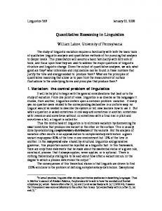
Figure 2.5: Hue Saturation Value (HSV) colour model. Graphic adapted from HSV model graphic by Jacob Rus from http://upload.wikimedia.org/wikipedia/commons/a/a0/Hsl-hsv models.svg (version 10.02.2010). Licensed CreativeCommons BY-SA http://creativecommons.org/licenses/by-sa/3.0/deed.en
preposition really applies, is likelier. In the example given above, people are more likely to say that A is neither “near” nor “far” from B, than that A is both “near” and “far” from B. The conclusion drawn from this is that people prefer an error of omission, where information is not presented even though it would be correct, than an error of commission with erroneous information in the spatial expression. In the image caption generation system presented later in this thesis (chpt. 6) this approach is mimicked, as spatial prepositions and geographical information are only included if the system estimates that they will improve the quality of the caption. The system will not try to force a spatial preposition. One approach to modelling these prototype effects is Gaerdenfors [72] “conceptual spaces”. In this model every concept is described via a set of properties and values. Each property defines a dimension in the conceptual space and the value specifies where along that dimension the concept lies. As an example the colour space would consist of the three dimensions hue, saturation and value. The concept “red” would then be anchored in concept space via the values hue = 0, saturation = 1, value = 12 . Using a similarity measure as described by Schwering [187] it is then possible to model the prototype effects as the distance in the conceptual space defines how close an object is to the prototype for that class. The “conceptual spaces” model has one shortcoming and that is that it requires all information to be quantitative and cannot handle qualitative aspects, which poses a problem when aiming to represent both the qualitative and quantitative aspects of spatial language. An alternative is to treat spatial language as a set of instructions as proposed by Miller and Johnson-Laird [153]. Thus a spatial expression “rocks near Stackpole Head” is translated into a procedural representation such as “near(rocks, Stackpole Head)”3 . A more complex expression is treated 2 Hue Saturation Value (HSV) is a colour model defined according to the colour cylinder in fig.
2.5, with hue as an angular dimension with values between 0◦ and 360◦ (red 0◦ , green 120◦ , blue 240◦ ), saturation as the distance from the centre with values between 0 and 1, and value as the vertical dimension with values between 0 and 1. 3 In this thesis “far” and similar spatial prepositions that indicate distant objects are not investigated, as in image
16
2
Background
as a nested set of such procedural statements so that “monument near Cardiff Castle, by the river“ would become “by(near(monument, Cardiff Castle), river)“. The statements can then be executed and in the processing of each procedure both qualitative and quantitative reasoning steps can be combined, making it possible to support more qualitative prototype effects and also purely quantitative effects such as distance or angle. Similarly Kuipers [123, 125, 124] uses a frame-like modelling language for route descriptions, each frame either describing a location and its properties or an action with its preconditions and effects. This is not strictly speaking a procedural, but a planning approach, however both offer the ability to combine quantitative and qualitative aspects. The choice between the two depends more on the context in which they are to be used than on the differences between the models. As the goal in this thesis is to interpret and generate spatial language, the procedural approach fits better and this is what the algorithms are modelled around. A further spatial language model that influenced some early ideas in the development of this thesis is Lakoff and Johnson’s “image schemas” [129, 103]. The core idea behind these is that since all humans live in the same world and are governed by the same physical constraints there is a set of universal concepts that underpin reasoning. Since most of these concepts are spatial in nature (path, surface, container, . . . ; see Johnson [103] for a full list) they have been used to underpin a variety of GIS research, such as spatial algebras for maps and room-space (Couclelis and Gottsegen [34], Rodriguez and Egenhofer [178]), interoperability (Frank and Raubal [58, 59]), wayfinding (Raubal and Worboys [171], Raubal and Egenhofer [170]), document retrieval (Fabrikant [50], Fabrikant and Buttenfield [51], and basic GIS concepts (Kuhn [122], Mark [144], Mark and Frank [61, 145]). Due to this it was initially planned to use an image-schemabased representation for the qualitative modelling processes, which would then be augmented with quantitative information. There is however one problem with the image-schema theory and that is that the original theory makes very strong claims towards the theory’s universality and that image-schemas are the actual human cognitive representational structure, claims that are based on only a small set of English-language examples and do not have any further supporting evidence. Due to this lack of empirical evidence the focus shifted to a procedural model closer to the Miller and Johnson-Laird ideas, as described above. However the algorithms retain some image-schema influence in that the various functions are named after the image-schema elements, as these provide a very clean set of labels. The procedural model also fits very well with the practical approach taken in this thesis, which focuses on the results and not the process, as will be discussed in more detail in the next section.
captions they would not provide a good location description and are thus not used.
2.4
Vagueness
2.3.1
17
The Practical Approach
As briefly touched upon in the previous sections, this thesis does not concern itself with the question of how the human spatio-linguistic reasoning system works. Instead the focus is always on replicating the human spatio-linguistic reasoning results, using whatever technical approach works best. The inspiration for this practical approach is that work in the computer vision area has shown that it is possible to create 3D representations of space, without requiring binocular vision (see Klein and Murray [115], Checklov and Gee [22], and Gemeiner et al. [74]). Thus a robot could navigate a 3D space, just as a human would, but without having the same internal processes and model. Similarly this thesis describes an approach to generating and interpreting language, where the results closely match a human’s, but with a different internal model and process. The results are human-like even though the system does not for example have a representation of the difference between “near” and “far” and how that affects humans’ construction of spatial language (see Kemmerer [110] or Diessel [41]). This decision to ignore the structure of the human spatio-linguistic reasoner also means that models that focus on the human spatial reasoning apparatus, such as those by Fauconnier and Turner [53], Knauff et al. [118, 119], or Olivier and Tsujii [158], had no influence on the work presented here and will thus not be discussed. Another influence was Egenhofer and Mark’s idea of “Naive Geography” [44], which at the basic level states that the rules and constraints of geographic reasoning, in any GI system that interacts with people, should be defined by what people believe to be true (everything is twodimensional, the earth is flat, maps are more real than reality4 ), even if this contradicts actual geographic reality. Following this idea the basic qualitative and quantitative rules and constraints of spatial language in image captions will be acquired directly from people using a set of human-subject experiments without recourse to any kind of a-priori constraints. As this thesis will show, when the context can be constrained sufficiently to acquire clean experimental data, then this simple, yet powerful approach can produce very good results that present a significant step to producing human-similar spatio-linguistic reasoning results.
2.4
Vagueness
As has been touched upon in the introduction, vagueness is a basic aspect of spatial reality (see Fisher [55], Parsons [161]). While man-made objects such as buildings, districts, countries have clearly defined boundaries, natural features such as coastlines, forests, mountains tend to have vague boundaries (Smith [194], Smith and Varzi [195]). Historically, as map-making 4 As
evidenced by the statement “When I get home, I need to check on the map where I went”.
18
2
Background
Figure 2.6: A broad-boundary representation of an island. The inner, dark area is the part of the island that is always above water and thus always part of the island. The lighter, grey area defines the broad boundary that is, depending on the tide, sometimes part of the island and sometimes not. The area outside the broad-boundary is the area that is never part of the island because it is always covered by the sea.
was done mostly by hand, the integration of vague information into the map was done via the use of symbol density, shading, colours, or any other method the map-maker wanted to employ. Unfortunately, the transition to computer-based map-making reduced maps to the crisp representations favoured by digital systems.
2.4.1
Qualitative Models for Vagueness
This preference for crisp representation meant that in Geographic Information Science (GIS) research the early models for reasoning about space were also crisp (see Randell et al. [169], Egenhofer [43], and G¨uting and Schneider [85]). However the problem of vague areas remained and extensions to the basic crisp models were proposed by Cohn and Gotts [31, 30], Clementini and DiFelice [27, 28] and Schneider [185]. These models replaced the original crisp boundaries with an extended boundary that represented the transition between the inner area where the phenomenon being described certainly applied and the outer area where the phenomenon did not apply at all any more. As an example, for a tidal sea-boundary, the delineation of the inner area would be drawn at the low-tide mark, while the boundary of the broad-boundary transition area would be drawn at the high-tide mark (fig. 2.6). From a qualitative point of view it is now possible to say which area is always sea, which is never sea, and the sea-ness in between is vague, without having to state how the vagueness between the two definite areas works in detail. The advantage of this approach is that it does not require any changes to the underlying computational architecture, as the original single crisp boundary is effectively replaced by two crisp boundaries. Another method for representing vague information that is similar to the broad-boundary models uses rough-sets as the underlying representation (see Ahlqvist et al. [2], Worboys [216] or
2.4
Vagueness
19
Bittner and Stell [9]). A rough-set consists of a pair of crisp sets, one representing the lowerbound and one the upper-bound. Those elements that are in the upper-bound set, but not in the lower-bound set basically define the elements of the broad-boundary in the broad-boundary models. One problem with the broad-boundary approaches to modelling vagueness is that they require a decision on where to place the inner and outer boundaries, a decision that is in most cases taken arbitrarily. An alternative model is proposed by Galton and Hood [70] called “anchoring” that allows for qualitative reasoning without having to specify arbitrary boundaries. The “anchoring” approach specifies certain constraints that hold for the relations between two or more objects, but does not specify any arbitrary, precise limits to the relations. As more information becomes available, these additional anchors will further constrain the location description until potentially the location is precise. To a certain degree the ideas in the caption interpretation system (sect. 5) follow this approach in that a qualitative model is constructed for the spatial descriptions in the caption, which is similar to the anchoring approach. The difference is that this qualitative model is then augmented with quantitative information to derive a quantitative model, to which quantitative precisification methods can be applied.
The qualitative models have been used to reason about both vague and crisp spatial information, but the primary focus in the qualitative reasoning work is on topological relations (contain, disjoint, overlap, touch, ...), which in image captions, with the exception of containment (“in”), play no significant role. Thus the discussion of qualitative reasoning will be short and Cohn and Hazarika [32] provide a more extensive overview of the field. Two areas where the qualitative reasoning work overlaps with the work in this thesis is linkage to spatial language (Shariff [190], Egenhofer and Shariff [45]) and the handling of cardinal directions (see Abdelmoty and El-Geresy [1], Frank [60], Papadias and Egenhofer [160], Clementini et al. [29], Goyal and Egenhofer [78, 79], Cicerone and DiFelice [26, 25]). Frank proposes that the cardinal directions should either be represented using a four-cone model consisting of only the four primary cardinal directions, or an eight-cone model that includes the intermediate cardinal directions (NE, SE, SW, NW). The experimental results presented in the next chapter will provide strong evidence that for humans the four-cone model is entirely sufficient, as in image captions the intermediate cardinal directions are not used in any significant number. Some work has been done on linking qualitative reasoning with quantitative aspects (see Kulik et al. [127], Hernandez et al. [93], Reinbacher [173]), but while these approaches try to include quantitative information they remain firmly grounded in a qualitative spatial reasoning approach, while the algorithms described in this thesis rely much more heavily on quantitative aspects.
20
2.4.2
2
Background
Fuzzy Models for Vagueness
The advantage of qualitative models is that they do not require modelling the quantitative aspects of how the vagueness works (see Freksa [62]). However when this quantitative aspect is of interest then the qualitative models are not sufficient. To enable such a quantitative representation it is necessary to move to a quantitative representation and a popular model is fuzzy-set theory5 [225]. Fuzzy sets use a membership function to represent to what degree an object is part of the set. Usually the range [0, 1] is used, with 0 representing classical non-membership and 1 classical membership. In between these two extremes, the membership value varies according to a pre-defined membership function that defines the fuzzy transition from non-membership to membership. It is the definition of this membership function that is one of the more difficult aspects of any fuzzy-approach, as a balance has to be found between a simpler membership function abstracted from the source data and a complex membership function that is directly derived from the phenomenon. Both approaches have their advantages, as the simpler membership functions tend to have better understood behaviour and properties when used with fuzzy operators, while the directly derived function provides a better representation of the vague phenomenon, the decision between the two approaches has to be made on a problem-by-problem basis (see Robinson [176], Bloch [10]). A number of fuzzy models have been devised for dealing with topological reasoning (Schneider [184, 183] and Winter [215]), geomorphological reasoning (Fischer et al. [56]), general spatial representations (Hwang and Thill [101], Tang [200], Pfoser et al. [163], Wang and Hall [212]) and most importantly linguistic reasoning (Schockaert et al. [186], Gapp [71], Robinson [177], Worboys et al. [217] [219], Gahegan [68], Fuhr et al. [67], Bloch [10]). The experiments described in these papers influenced the design of the experiments that will be described in the next chapter. Especially influential was the work by Schockaert et al. [186] which illustrates that by using a focused corpus (in their case of hotel websites) it is possible to derive a fuzzy representation of an arbitrary spatial phrase such as “within walking distance”, an approach that was used to derive an initial overview of how spatial prepositions were used in image captions (sect. 3.1). The Worboys [217] and Robinson [177] experiments and the work by Fisher and Orf [54] showed that it is possible to acquire fuzzy representations directly from people using a map-based approach, which formed the basis for the human-subject experiments (sect. 3.2 and 3.3). An interesting aspect is that they describe varying levels of success in their experiments. While Worboys and Robinson report that they have created multi-person fuzzy 5 There
is also the possibility of using an approach based on supervaluation (see Bennet [6] or Kulik [126]), which allows for the creation of a set of boundaries that describe the gradual transition from the definite to the definitely-not area, similar to iso-lines used to represent height on conventional maps. The fuzzy methodology seems to be more frequently used, thus is given prominence. Supervaluation is also sometimes seen as belonging more to the area of qualitative models, however as it will not be discussed further the question of what area it belongs to is not relevant here.
2.4
Vagueness
21
models for “near” in the respective contexts (Worboys in the campus context, Robinson in the inter-town context), Fisher and Orf state that the results of their experiment show such a large amount of variation that they cannot be used to create a formal representation of “near” (again in the campus context). The results presented in this thesis also show a lot of variation, but they also indicate clear trends and these make it possible to create models for representing the spatial prepositions’ vagueness. A side-effect of using a fuzzy-based approach is that, as Altman [3] illustrates, the detailed representation of the vague phenomenon can be retained throughout the spatial reasoning process and only at the final decision point is the fuzzy representation reduced to a true/false decision, a decision that with the previous qualitative representations has to be taken much earlier in the reasoning process. The concept of maintaining as much spatial information as far through the spatial reasoning process as possible is an approach that is taken throughout this thesis. Both the caption interpretation and generation systems maintain as much information as possible until in the final stage of their reasoning processes they select the final answer from the more detailed representation. In addition to creating a richer representation this also allows for a simpler implementation, which in turn makes the implementation more robust with respect to errors in the underlying data.
2.4.3
Field-based Models for Vagueness
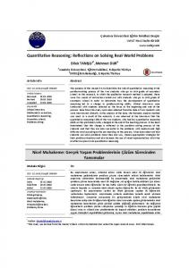
The various fuzzy representations are very powerful tools for representing vague knowledge, but to use them it is always necessary to represent the vague knowledge as one or more membership functions and in the case of multiple membership functions the methods for combining them need to be specified, which can be quite difficult. To avoid this difficulty the vague data can be represented using a field model, which maps each pair of coordinates to a vague value6 (see Liu et al. [141] or Laurini and Pariente [132]). Fields represent geographical knowledge as a continuum of values, contrasting with object-based representations that split geographic space up into a set of more or less clearly delineated objects (see Couclelis [33], Goodchild [76], Galton [69]). As an example a field model could use a matrix of water depth values to represent a lake, while an object model would use a polygon to define the lake’s boundary by fiat (fig. 2.7). However, the two concepts are not exclusive, there are cases where either model can be used, cases where an intermediate model such as the one by Erwig and Schneider [46] is most applicable, and also cases where one of the two models provides clearly better results. In general fields tend to be better suited to representing spatial information, while an object model makes the manipulation of the individual spatial objects easier. This is due to the 6 Fields
can of course also store non-vague data, but in this thesis only the representation of vague data is of interest.
22
2
Background
Figure 2.7: The same lake represented as a field and as an object. The figure on the left shows the fieldview, which represents the lake via the water-depth (the darker the colour, the deeper the lake). The figure on the right shows the object view where the lake is defined via a boundary that represents the modeller’s choice as to where the lake ends.
field’s continuous nature, which is much closer to reality than an object representation and thus the field can represent reality more easily and with higher fidelity. On the other hand simple manipulations such as changing an attribute or the extent of a feature (whatever this feature may be) are much easier if the feature is represented as an object, as in this case the change is applied to that specific object, whereas in a field representation the change would have to modify a potentially large part of the field. In this thesis a hybrid approach is used where a fieldbased representation is employed to represent the quantitative aspects of the spatio-linguistic reasoning process, while the qualitative aspects are represented using an object-based model. In GI systems the object view is predominant, but there are also a number of field-based approaches, which are all grounded in the desire to represent spatial data that has no clear boundary, mostly data derived from spatial language expressions. Nishida et al. [157] and Yamada et al. [223, 224] use a field-based approach to determine the precise location described by a spatial expression. Based on the spatial expression they construct individual fields for each spatial preposition and then interpreting the fields as energy functions locate the lowest-energy point, which they define as the location described by the spatial expression. Focusing on areas instead of single locations, Wieczorek et al. [214] describe a system that quantifies the uncertainty of a spatial description and creates a circular area defining the described location. This approach is extended by Guo et al. [84] and Liu et al. [140] with the result that the final area no longer has to be circular. Linguistic descriptions of space are also of interest to the robotic navigation field (see Mukerjee et al. [156]), as they would allow for a simpler interface between humans and robots. Fields have also been used to model non language-based phenomena such as Brown’s [13] model for forest types, which uses kriging to interpolate a continuous field from point measurements, a method that is also used to instantiate fields in this thesis. On the generation side, Schirra [181] uses a field-based approach to generate descriptions of spatial configurations of players on a football pitch, similar in effect to the work on generating spatial descriptions of image locations described in chapter 6.
2.5
Conclusion
23
The various approaches use different functions to describe the uncertain information they are representing, none of which are based on how people actually interpret spatial expressions, and this grounding in actual human use of the spatial prepositions is what sets the work in this thesis apart from existing work. While Mukerjee et al. do investigate human aspects, it is unclear how these filter back into the models they have defined. One interesting aspect in their work is that they report that the size of the ground and figure objects of a spatial preposition have no influence on how the spatial preposition is interpreted, which directly contradicts the work of Morrow and Clark [155] who report a significant influence of the relative sizes of figure and ground objects. Potentially the different contexts in which the experiments were performed explains the differences, however in the human-subject experiments presented in this thesis the relative sizes have been normalised to avoid any potential influences. It is also important to note that the work of Wieczorek et al., Guo et al., and Liu et al. define the vagueness as “uncertainty”. This implies that it is in theory possible to determine a precise location, if the uncertain aspects of the spatial expression could be made certain. In this thesis it will be argued that the vagueness in spatial expressions is a vagueness that is inherent to spatial language and that it is impossible to remove this vagueness. If a specific location is described as “a few kilometres north of Merthyr Tydfil” then this expression is inherently and immediately vague and not uncertain, as the act of using spatial language to describe a location leads to a loss of information that is non-reversible. Only the person who specified the location description can find the precise location, but even they have to rely on non-linguistic information such as their spatial memory.
2.5
Conclusion
This concludes the overview of the main areas on which the work in this thesis builds. There are of course more specific links between existing research and the work in this thesis and these will be discussed throughout the thesis when and where they become relevant.
24
2
Background
3 Vague Spatial Language
Spatial language is one of the primary methods for communicating spatial information. It is used to describe the location of an object (“the pen is next to the book”), give directional instructions (“turn left at the next intersection”) and to retrieve objects (“can you pass me the glass by the jug”). It can be used in different contexts (“the pen next to the book”, “the tree near the house”, “Reading west of London”), in different contexts (“turn left” as a driving instruction, as an instruction in a supermarket, as an instruction when playing a board-game) and above all due to it qualitatively describing quantitative relations, it is vague. Philosophically, vagueness is described as the problem of where to draw the line in the Sorites paradox (Fisher [55]). When do a few sand grains make a heap, or in geographic terms, when is a geologically up-thrust area a hill, when does it become a mountain, where is the boundary between the terms and does such a boundary exist at all. This problem translates into spatial language as well. When is an object “near” another object, at what point does it become “next to” it. How people define these boundaries is the focus of this chapter and as the experiments described in this chapter will show, this is not an issue of imperfection (Worboys and Clementini [218]) or imprecision (Guo et al. [84] and Liu et al. [140])). Spatial language is inherently vague, people are aware of this vagueness and are able to express it in the experimental settings. In addition to this inherent vagueness there is also the vagueness that is introduced by interparticipant disagreement (see Robinson [177]) due to the participants having different mental models of how the spatial prepositions’ work quantitatively. Next to the inherent vagueness and the inter-participant disagreement type vagueness there is also the vagueness introduced by contextual factors such as the relative sizes of two objects being related to each other or the activity within which the relation is embedded. The experiments in this chapter will look at the first two sources of vagueness, while the contextual vagueness has been eliminated as far as possible by presenting the specific context of describing the location of a photograph in an image caption, a process that implies a specific size of ground toponym and is relatively static as will be explained in more detail later. To be able to quantify this vagueness three experiments have been run. The initial experiment
26
3
Vague Spatial Language
used a data-mining approach to provide an overview of how spatial language is used in image captions, but the problem with data-mining is that it is very hard to determine why the results look like they do and this then influenced the development of the two human-subject experiments. The difficulty with human-subject experiments lies in focusing the experiment so that the results are not too heavily biased by the experiment setting. An example is that in both human-subject experiments maps are used to remove any influence caused by participants not knowing where the places used in the experiment are, but at the same time the use of such a map influences the results (Linden and Sheehy [139]). The final decision was that the influence caused by the lack of spatial knowledge was less desirable than the map influence and thus a map was included1 . There were a number of such choices and the reasons for each choice will be stated. The studies presented here are not the first to investigate spatial knowledge via human-subject experiments, as people’s spatial knowledge is a very rich source of information (Mark et al. [147]). A number of studies have looked at quantifying spatial preposition use (Fisher and Orf [54], Robinson [177], Worboys [217]) and vague places (Montello et al. [154] and Evans and Waters [48]). The designs of these studies influenced the design of the experiments described here and the results are compared to their results. While the first human-subject study was run off-line as a set of traditional human-subject experiments, the second human-subject study was run as an on-line application. The main advantage of an on-line experiment is the vastly higher number of participants that can be accommodated (∼1000 in the on-line experiment compared with between 23 and 72 participants in the traditional, off-line experiments), but it also introduces the problem that the participants are not in a controlled environment when they participate in the experiment (see Schmidt [182] or Wyatt [220]). In the end the large number of participants provides high confidence in the results, a view that is supported by a number of studies that show that the results of on-line and off-line experiments are comparable (Krantz et al. [120], Buchanan and Smith [15], Zhang [226]). A general problem with most studies is that they are based in universities and as such draw heavily on the student population as experimental subjects, with both Smart [188] and Buchannan and Smith [15] showing that roughly 80% of all psychology studies are performed on undergraduates. When inviting participants to the studies both students and staff were invited and while the majority of participants were undergraduates the inclusion of staff should provide for more reliable results2 . In the analysis two contexts are distinguished. The first is the rural context where the majority of toponyms are small towns, villages, other small settlements and natural features such as 1 Also
using maps as a primer has been shown to improve spatial reasoning performance (Davies [40]) way at least the approach follows established best-practices, regardless of how good these are.
2 Either
3.1
Data-mining Spatial Language in Image Captions
27
lakes and mountains. The quantitative aspects at this context are investigated in the data-mining experiment (sect. 3.1) and rural-context experiment (sect. 3.2). The second context is the urban context where the majority of toponyms are points-of-interest such as buildings, monuments, parks and roads, which will be investigated in the urban-context experiment (sect. 3.3).
3.1
Data-mining Spatial Language in Image Captions
To develop an initial understanding of the quantitative aspects of spatial language as used in image captions, an existing, large, geocoded image caption data set was analysed. This data set was acquired from the Geograph project3 , an open-participation project that aims to provide a representative photograph for each square kilometre of the United Kingdom and Ireland. A dump of roughly 350,000 image captions and locations forms the basis for this analysis. Due to the aim of providing representative photographs the images tend to be ground-level and panoramic for rural areas and of buildings or roads in urban areas, with captions such as “Footpath at Pirbright”, “Farmland near Garthorpe” or “Lambeth Palace from Lambeth Bridge”, which are rich in spatial language (tab. 3.1). The Geograph project provides a quite specialised data-set and a more general image caption data-set such as could be provided by mining Flickr4 was considered. However the initial data-acquisition from Flickr showed that as a source for quantitative data on spatial language it was not well suited. The amount of spatial language used is relatively low (many photos have no caption at all), the API for querying Flickr does not make it easy to restrict the images to the UK, and the geocoding quality is very variable with frequent errors of up to two or three kilometres observed. The low spatial language incidence and geocoding quality issues resulted in the decision not to include Flickr in the analysis, as the focus is on spatial language and if the image location does not provide a trustable ground-truth then any conclusions drawn from such data hold little value. The Geograph data was analysed along three separate lines. Quantitative analysis of how frequently the spatial prepositions are used, quantitative analysis of how the spatial prepositions “near” and the cardinal directions are used, and a qualitative analysis of the syntactical patterns found in image captions. As with many on-line data sources based on public participation, there is a bias in the data as a small group of prolific contributors provide the majority of the data. In the Geograph data-set analysed here, roughly 90% of the image captions were produced by about 2% of the contributors. To avoid this bias affecting the qualitative pattern analysis only one caption per participant was used. After the analysis of the reduced set was completed the 3 http://www.geograph.org.uk 4 http://www.flickr.com
- An online photo-sharing site
28
3
Vague Spatial Language
The B3309 turning to Ludgvan Summit track, Scawd law Porth Chapel Beach Branscombe Beach and Beer Head Looking North along Dark Lane Barton Aqueduct Fields between Trayslefield farm and Manor farm Wing Road near Glaston Lignatraw Townland Dent Dale Table 3.1: Ten captions chosen randomly from the Geograph data-set to illustrate the range of captions available.
Spatial preposition at near to on from in north west east south
Frequency 21754 18589 15476 13698 12886 10753 5336 5230 4763 4756
Table 3.2: Top-ten most frequent spatial prepositions in the Geograph data with their frequencies
full set was analysed in the same way and the same patterns were identified with the same relative frequencies. From this the conclusion is drawn that the participant bias does not overly bias the analysis results even if the full set of data is used. This made it possible to use the full set of image captions in the quantitative analysis.
3.1.1
Spatial Preposition Frequency
Before analysing the spatial preposition uses in detail a quick analysis of their use-frequency was performed (tab. 3.2). The frequencies were calculated by counting the frequencies of all words in the Geograph corpus and then from that frequency list filtering out the spatial prepositions. As can be seen in the table “at” and “near” are the most popular spatial prepositions, followed by “to”, “on”, and “from” which are mostly used to describe paths and roads. The next spatial preposition is “in” followed by the cardinal directions. Overall the total number of captions in which a spatial preposition is used is about 85,000 out of a total of roughly 350,000 captions, indicating that in about three quarters of all captions
3.1
Data-mining Spatial Language in Image Captions
29
a set of one or more toponyms is a sufficient description of the image’s locations. This is further substantiated in section 3.1.3 where the structural analysis identifies two frequently used patterns that do not use any spatial prepositions at all. The list of spatial prepositions in the frequency table is roughly as would be expected, however one set of spatial prepositions is absent from the list and those are the intermediate cardinal directions (north-east, south-east, south-west, north-west). For these the total sum of uses in the 350.000 caption set is 630. Compared to the total of 20.085 for the primary cardinal directions it is evident that in normal caption language the intermediate cardinal directions play no significant role and can be excluded from future analysis. This is in contrast to the results of experiments by Zimmer et al. [227], who show that when describing the position of an object in table-top space, the intermediate directions are used more widely than the primary directions. However their experiment analysed the uses of left/right and above/below and the participants were instructed to provide a very precise description so that a second user could replicate the precise configuration of the figure and ground objects. It is highly likely that the difference in results is due to this requirement for a very precise description, which in image captions, where the scale is much larger, is simply not necessary. For images the precision required for locating an image can be provided by the four primary directions. Based on the use frequencies the spatial prepositions, that would be analysed in more detail, were selected. For the initial data-mining analysis in the next section these are “near” and the cardinal directions. The other spatial prepositions were ignored for the moment as the path related prepositions (“from”, “to”, “on”) did not fit the analysis technique and with “at” there were also difficulties geocoding the ground toponyms, as they often referred to very local toponyms that could not be found in the gazetteers or not uniquely disambiguated if there was more than one place with such a name. The road-related prepositions are included in the humansubject experiments (sect. 3.2 and 3.3) and “at” is investigated in the urban context (sect. 3.3), where further interesting, but harder to model, aspects of the interpretation of “at” became apparent, which meant that it was most likely unsuitable for the automated data-mining based analysis approach. The relative frequencies will also used in the caption generation to weight the choice of spatial preposition if more than one spatial preposition can be used to describe a location (sect. 6.5).
3.1.2
Spatial Preposition Use5
After identifying the most frequent spatial prepositions, “near” and the cardinal directions were analysed quantitatively in more detail. The first step in this analysis is extracting their uses 5 An
early version of this section has been published in Hall and Jones [89]
30
3
Vague Spatial Language
from the image captions. GATE [36] is used for part of speech tagging and the identification of spatial relations. Toponym identification is handled by a simple rule. Words starting with an upper-case letter are determined to be candidate toponyms, excluding stop words such as “A” or “The”. Multiple, consecutive candidate toponyms are aggregated into one multi-word candidate toponym. This rule identifies the majority of toponyms, especially toponyms for populated places. The only group of toponyms that this method does not identify are those using generic toponym classes such as “station” or “church”, but there is a very limited number of such generic names in frequent use, and they can be handled by a simple rule that states that if a candidate toponym is followed by one of these toponym classes, then the class is appended to the toponym. In the end this rule was not implemented, as difficulties with correctly geocoding such toponyms meant that the analysis used only populated places such as villages and small towns, which are easier to geocode correctly. The tagged captions are then matched against patterns of the form “ ”, with the optional image topic usually describing the content of the image. The hypothesis is that the GPS coordinates of the camera location, as stored in the image meta-data (representing the spatial preposition’s figure location), and the location of the toponym (the spatial preposition’s ground toponym) matched by the pattern form one valid use of the spatial preposition. Multiple uses of each spatial relation are used to build up a quantitative model. The toponyms are geocoded using the Geonames.org service6 , which returns a point representing the centre of the toponym location. Toponym disambiguation was based on accepting only exact toponym matches and selecting the first if there were multiple exact matches. As the distances involved in the spatial language of image captions tend to be short (mostly less than 5km), a reference to the wrong toponym is immediately clear as a statistical outlier. A hard limit of 12km is enforced on the distance, filtering out the incorrect toponym disambiguations. For each of the patterns the GPS co-ordinates of the image and the location of the toponym are combined to calculate the angle and distance from the ground toponym to the image location. Combining these distance/angle pairs into sets makes it possible to create distribution plots based on a common ground location, as shown in figure 3.1. The main analysis is then based on these sets of distance/angle pairs. As this method combines distance and angle data from multiple captions, it is necessary to guarantee that the size of the ground toponyms involved in all captions is the same. The area “south of” a point of interest such as a church will have a different extent to that “south of” a town or village. The Geonames.org service in addition to the location of the toponym also provides information on the toponym’s type and in the data presented in this analysis only toponyms of the type 6 http://www.geonames.org
3.1
Data-mining Spatial Language in Image Captions
31
Figure 3.1: Figure locations for the cardinal direction “north” plotted from a common centre, representing the ground location (black x).
populated place were used. As will be explained subsequently, this corresponds in practice to a characteristic size of place.
Near Results In total 4607 data points were analysed. The distances (fig. 3.2) calculated varied between 20m and 11930m, with a mean of 2190m and a median of 1800m. The inter-quartile range is 1630m, with the first quartile at 1140m and the third quartile at 2770m. Points with a distance of over 5200m are classified as outliers. The angle was analysed using a circular mean (see Jammaladaka and Sen Gupta[102]), with a value of 342◦ . This indicates, as can also be seen in figure 3.3, that while all possible directions are used in the “near” relation, there is a slight preference for choosing a toponym that lies south of the location being described.
Discussion The data clearly show that the distances involved in the “near” relation are not very high. This is probably due to a combination of factors. One is that there is a distance limit of a about ten kilometres where places are “near”. The other is that in addition to this upper bound, in roughly three quarters of all cases there is a ground toponym within less than three kilometres that is sufficiently well-known to be used to describe the image’s location. One aspect the distance distribution does not take into account is the actual extent of the ground toponym. As the Geonames.org service only returns a point representation for the ground toponym, the distance from that point to the boundaries of the ground toponym is included in the distances calculated. Unfortunately the strength of this effect cannot be quantified from this data, but reasons why the influence does not introduce any significant error are discussed later.
32
3
Vague Spatial Language
Figure 3.2: Histogram showing distance distribution for “near”, bars calculated at 500m intervals.
Figure 3.3: Stacked circular angle distribution for “near”. Angles shown are calculated from the ground to the figure location.
3.1
Data-mining Spatial Language in Image Captions
33
For the angle distribution the assumption had been that angles would be distributed evenly across the full 360◦ arc, but the data show that there is an increased number of points with angles near north. This implies that when using “near” to describe a location, there is a preference for choosing a ground toponym that lies south of the location being described (the angle data shows the angle from the ground toponym to the described location). Watson’s test for circular uniformity shows that the data are significantly (p < 0.01) non-uniform, so there is an actual effect to be seen here and it is not just a chance distribution. One possible explanation is that when viewed on a map the ground toponym will be below the photo location being described. Thus when used in the image caption it provides a virtual support on which the location being described can be placed using the “near” preposition. Clearly this support relationship is not a necessary one however, as half the data points are in the remaining two thirds of the full arc. Another possible explanation might be that due to the sun being in the south there is a bias towards taking photos in a more northerly direction, which then influences the toponym selection when writing the image caption. At this point no definitive explanation can be given for this effect, especially as the effect is not visible in the human subject experiment described in the next section ( 3.2). It has also been investigated, whether angle and distance correlate. To make it possible to apply a linear model the angular data is transformed into a linear representation using equation 3.1. This is possible as the question is whether changes in the distance are correlated with angle changes as the angle moves from north to south, irrespective of whether the angle points to the east or west. The angles in the transformed data are in the range [0, 180] with 0 indicating north, 180 indicating south, and 90 indicating either east or west. A linear model distance = a + b · angle has been fitted to the transformed data, and with a = 2272.386 and b = −1.103 and shows significance at p = 0.0159. This seems to indicate that when the ground toponym location is south of the described location, it can be slightly further away. However the residual standard deviation of the model is 1590m, with a difference between north and south of only 200m, thus the statistical significance of this model is most likely only an artefact. Due to this the conclusion must be that the linear model fits, but is without value and in practice the angle does not influence the distance, as will be substantiated in the human-subject experiment. ( trans f orm(angle) =
angle angle ≤ 180 |angle − 360| angle > 180
(3.1)
Cardinal directions Results A total of 1081 data points were analysed for the cardinal directions (307 north, 330 south, 225 east and 219 west).
34
3
Vague Spatial Language
Figure 3.4: Box plot of the distances by cardinal direction (east, north, south, west). Clearly visible is that “east” and “west” are very similar, while “south” is significantly different. Also visible here is that all points over about 4 to 5km are classified as outliers (empty circles).
Distances for “north”, “east” and “west” varied between 120m and 11940m, with means between 2080m and 2220m. Medians varied between 1510m and 1920m, with the inter-quartile ranges between 1240 and 1590m. The distances calculated for “south” varied between 40m and 11360m, with a mean of 1800m and a median of 1390m (fig. 3.5). The inter-quartile range is 1310m, with the first quartile at 820m and the third quartile at 2130m. The differences in distribution are visible in figures 3.4 and 3.5. The north angle data shows a slight shift to the west, with a mean of 355◦ , whereas the south data is almost perfectly south with a mean of 181◦ . The east distribution is rotated by 23◦ towards north with a mean of 67◦ , while the west distribution is rotated north by 16◦ with a mean of 286◦ .
Discussion Just as in the “near” case, the distances involved in the cardinal directions are not very high, probably due to the same reasons as described in the “near” section. Comparing the individual cardinal direction distances using ANOVAs showed that the “east” and “west” distributions can be considered basically equivalent (p > 0.9). While “north” shows no significant
3.1
Data-mining Spatial Language in Image Captions
35
Figure 3.5: Distance histograms for the “north” and “south” distributions. The differences in the distribution shapes between “north” and “south” are clearly visible.
36
3
Vague Spatial Language
Figure 3.6: Circular plots for all four cardinal directions.
3.1
Data-mining Spatial Language in Image Captions
37
differences from “east” and “west”, the median and inter-quartile distances are slightly higher for “north” indicating that with a larger sample a statistically significant difference might become apparent. The “south” distribution on the other hand shows significantly shorter distances (p < 0.01), when compared to the three other directions, meaning that three different models for distances of cardinal directions need to be distinguished. These patterns can also be seen in the box plot in figure 3.4. The angle data show a similar pattern, with “east” and “west” very similar. The “east” angles were mirrored across the north-south axis and Watson’s two sample test applied, showing no significant differences between the “east” and “west” angle distributions. An interesting aspect about these two distributions is that they both show statistically significant rotational shifts towards north, when compared to the same distributions centred on the east-west axis. Whether this rotational shift is caused by a subconscious error in the understanding of the east/west directions or whether it is an artefact caused by the preposition selection process, or whether some other effect is the reason cannot be determined at this point. Neither the “north” or “south” distribution show any similar kind of effect, however the “south” distribution is wider filling the gap between the “east” and “west” distributions. This indicates that it is likely that the effect is due to the preposition selection process as in total the four cardinal directions completely cover the whole 360◦ arc. Both the angle and distance data for the cardinal directions suggest that three separate models are required to describe the directions. One model each for north and south, and a third model to describe east and west. As in the use-frequency analysis above, the results differ from those in Zimmer et al. [227]. They reported that the primary directions were used only for a very small sub-set of the angles around the central angle of each primary direction. The intermediate directions were used to fill the gaps that this created. When combined with the results seen in the analysis of the cardinal directions, the conclusion must be that when the intermediate directions are not used or required, then the primary directions expand to cover a much larger range of angles to fully cover the whole 360◦ arc.
Discussion The extent of the ground toponym has an influence on the distances calculated and while the restriction to populated places reduces this influence, populated places also cover a wide range of sizes and in principle this could have a strong influence on the results. I believe that in the case of spatial relations as used in image captions, the act of captioning tends to rely on very local information and this acts as a restricting force on the size of the toponyms used. This
38
3
Vague Spatial Language
is supported by the actual distribution of distances (fig. 3.5) obtained and by observation of a sample of the actual ground locations used. If larger places were frequently used as the ground toponym, then to end up with the distributions that the data show, the distances used with the spatial preposition would have to be inversely proportional to the extent of the place. In other words the larger the extent of the ground toponym, the shorter the distance where places are described as “near” the ground toponym. This is highly unlikely and it is much more likely that in image captions only local and small places are used as ground toponyms, creating a characteristic size of toponyms used in image captions. This influenced the context of the first human-subject experiment (sect. 3.2). The main problem with the data derived from the Geograph data set is that there are a number of factors which influence the data, but which cannot be quantified. These include the effects caused by the contention of multiple spatial prepositions for describing one location and also errors introduced by the geocoding, incorrect parsing of the image caption and data acquisition errors. To create a cleaner and more stable model, a human spatial experiment was designed and executed, providing a spatial data set that was collected under controlled and focused conditions (sect. 3.2).
3.1.3
Structural Analysis of Captions
The quantitative analysis in the last section looked for simple patterns of the form and used those patterns to extract the required spatial information from the captions. For the caption interpretation and generation algorithms presented later in this work (sect. 5 and 6), a more complete understanding of the structures involved in image captions is required. To this end a syntactical and statistical analysis of image caption language has been undertaken. The structural analysis is based on collocation frequency, which represents how often certain word combinations appear in the text corpus that is being analysed. While a pure word collocation analysis in image captions can produce interesting results, the problem is that there is so much variation in how place-names are structured and how they are combined with adjectives and syntactic elements such as determiners. This variation amounts to noise that obscures the structural pattern signals. To avoid this the statistical analysis is based on a syntactically tagged part-of-speech (POS) representation of image captions and not directly on the image captions. Table 3.4 shows an example caption and its POS tags and it is collocations of these POS tags (fig. 3.3) that form the basis for the structural analysis. The analysis process uses a semi-automatic approach where the collocations are calculated automatically and sorted by frequency. Based on the most frequent collocations a set of generali-
3.1
Data-mining Spatial Language in Image Captions POS tag NN NNP IN TO DET CC JJ POS VB RB
Description Noun Proper noun - name Preposition The word “to” Determiner Conjunction Adjective Possessive ’s Verb Adverb
39 Example hill Watford near to the and old ’s looking quickly
Table 3.3: Basic part-of-speech (POS) tags used in this thesis, with examples
NN NN IN NNP Railway bridge near Ardvorlich Table 3.4: Example caption taken from the Geograph data set and the POS tags assigned to each word. NN - noun, IN - preposition, NNP - proper noun.
sation rules are then created manually. In theory it might be possible to create the generalisation rules automatically, however to ensure that the automatically created rules are sensible the algorithm would have to be provided with an extensive understanding of English grammar, which defeats the goal of having a fully automatic process. Instead the semi-automatic approach plays to the strengths of both computers and humans, with the computer able to quickly calculate the collocations and the human able to easily spot and create the correct generalisation rules. Additionally the human can apply their knowledge of English grammar to the generalisation process and in the process create better and simpler generalisation rules than possible with a fully automatic approach. Calculating the POS tag collocations for the set of Geograph captions produces the collocation distribution7 shown in table 3.5. As can be seen in that table, the most frequent collocations are noun - noun (NN, NNP) combinations, preposition (IN) - noun patterns and noun - comma patterns. The POS tagging has reduced but not eliminated the amount of variation. To further reduce this variation the most frequent collocations are used as generalisation rules (tab. 3.6). These combine various noun combinations into noun-phrases (lines 1 to 4), create prepositional phrases (line 5) and comma separated phrases (line 6). After the generalisation rules are defined the process starts from the beginning, except this time the generalisation rules are applied first and then the collocations are calculated using the partially generalised captions (tab. 3.7). 7 As
mentioned before to avoid a bias being introduced by a small group of frequent contributors producing most of the captions only one caption per contributor was considered. This reduces the number of captions from around 350000 to 580.
40
3
Vague Spatial Language
Tag 1 Tag 2 Frequency NNP NNP 632 IN NNP 149 , NNP 110 NNP IN 109 NNP , 109 NNP NN 72 DET NNP 68 NN IN 62 IN DET 53 NNP CC 30 Table 3.5: Top ten collocations derived from 580 captions (out of a set of ∼350000 captions, but only one caption per user considered).
Tag 1 Tag 2 Tag 3 Generalisation NNP NNP NPhr NNP NN NPhr NN NNP NPhr NN NN NPhr IN NPhr IPhr NPhr , NPhr CommaPhr Table 3.6: Generalisation rules created based on the first collocation list. The central rule is the generalisation of nouns into NPhr (noun phrase) elements. Additionally based on the collocations of NNP with prepositions (IN) and commas generalisation rules for prepositional phrases (IPhr) and comma-delimited phrases (CommaPhr) are created.
NPhr IPhr Railway bridge near Ardvorlich Table 3.7: Example caption taken from the Geograph data set and the POS tags after the first generalisation rules have been applied.
3.1
Data-mining Spatial Language in Image Captions
41
Figure 3.7: Incorrect syntactical tree structure generated by applying the rules from left to right.
Figure 3.8: Correct syntactical tree structure generated by applying the rules from right to left.
The generalisation rules are applied from right to left (see section 5.2.2 for details on the generalisation algorithm in listing 5.1). If the rules were applied from left to right then a caption such as “The old gate house” would result in the syntactical tree structure shown in figure 3.7. This structure would incorrectly imply that the adjective (JJ) “old” belongs to the noun (NN) “gate” instead of the combined noun “gate house”. Similarly the determiner (DET) refers to the whole noun phrase (NPhr) and not just the “old gate”. Applying the rules from right to left produces the correct syntactical tree (fig. 3.8). After the generalisation rules are applied the collocations are calculated again, resulting in the distribution in table 3.8. The big change is that there are a lot of captions that consist only of a noun phrase. Also three further patterns emerge, namely a noun phrase and a prepositional phrase, a noun phrase and a comma phrase and two noun phrases joined via a conjunction (CC). The first pattern will be generalised (tab. 3.9) as a FigureGroundPhr because the spatial preposition relates two noun phrases which play the semantic roles of figure and ground (“Pontsticill reservoir near Merthyr Tydfil”). The noun phrase and comma phrase will be generalised as a ContainPhr as they define a toponym hierarchy (“Roath Park, Cardiff, Wales”). Finally the conjunction is generalised as a conjunctive phrase (ConjPhr) which in turn is generalised to a NPhr (noun-phrase) so that it can be integrated into the other generalisation rules. The next iteration of the collocation calculation (tab. 3.10) already shows the basic pattern that the collocation analysis will show, namely that there are three basic patterns that make up most captions (NPhr, FigureGroundPhr, and ContainPhr). Also a few further small variations in noun phrases show up, such as the use of the possessive s and adjectives, which are simply integrated into the NPhr (tab. 3.11).
42
3
Vague Spatial Language
Tag 1 Tag 2 Frequency NPhr 202 NPhr IPhr 120 DET NPhr 105 NPhr CommaPhr 82 IN DET 53 NPhr IN 51 CC NPhr 28 NPhr CC 27 JJ NPhr 26 POS NPhr 24 Table 3.8: Top ten collocations derived from 580 caption after the first generalisation rules have been applied (out of a set of ∼350000 captions, but only one caption per user considered).
Tag 1 Tag 2 Tag 3 Generalisation DET NN NPhr DET NNP NPhr DET NPhr NPhr NPhr IPhr FigureGroundPhr NPhr CommaPhr ContainPhr NPhr CC NPhr ConjPhr ConjPhr NPhr Table 3.9: Generalisation rules created based on the second collocation list. The second set of generalisation rules expand the flexibility of the NPhr handling by integrating determiners (DET), adjectives (JJ) and possessive s (POS). The big additions are the combination of a NPhr and a IPhr to the FigureGroundPhr and the ContainPhr representing containment hierarchies.
Tag 1 Tag 2 Frequency NPhr 224 FigureGroundPhr 82 ContainPhr 58 NPhr POS 22 NPhr IN 16 JJ NPhr 51 POS NPhr 14 ConjPhr 14 DET JJ 13 NPhr VB 12 Table 3.10: Top ten collocations derived from 580 caption after the first two sets of generalisation rules have been applied (out of a set of ∼350000 captions, but only one caption per user considered).
3.1
Data-mining Spatial Language in Image Captions
43
Tag 1 Tag 2 Tag 3 Generalisation JJ NN NPhr JJ NNP NPhr JJ NPhr NPhr NPhr POS NPhr NPhr Table 3.11: Generalisation rules created based on the third collocation list. The second set of generalisation rules expand the flexibility of the NPhr handling by integrating adjectives (JJ) and possessive s (POS).
Tag 1 Tag 2 Frequency NPhr 240 FigureGroundPhr 100 ContainPhr 62 ConjPhr 16 NPhr . 11 TO NPhr 10 : NPhr 10 NPhr VB 10 NPhr IN 9 NPhr RB 8 Table 3.12: Top ten collocations derived from 580 caption after the first three sets of generalisation rules have been applied (out of a set of ∼350000 captions, but only one caption per user considered).
The final collocation table (tab. 3.12) shows little change for the most frequent patterns. Two more generalisation rules can be extracted (tab. 3.13), treating the word “to” as a preposition8 and generalising anything that contains a verb (VB) as a full sentence, however these play only a minority role and will not be used in the caption interpretation or generation. From the final collocations it is also possible to see cases where the POS tagger created an incorrect tag or where the caption processing failed in some other way (tab 3.14), by looking at the words in the NPhr/. and NPhr/IN collocations. It is unclear why the words in the NPhr/. case are assigned to these POS tags and whether in the NPhr/IN case these are captions that 8 The
word “to” is usually marked up as TO by POS taggers as it is used both prepositionally and also as the infinitive marker. As the infinitive case is not particularly likely in image captions, it is simply generalised as a preposition and can then be treated as such by the other generalisation rules.
Tag 1 Tag 2 Tag 3 Generalisation TO IN * VB * Sentence Table 3.13: Generalisation rules created based on the fourth collocation list. The rules are for completeness sake, but play no role in further analysis or processing.
44
3
Tag . IN
Vague Spatial Language
Words Chait, Ghrunnda, Gest, !, ford, Drain, TONGWYNLAIS, allotments, Dailthean, Locks on, in, across, at, from, of, with, footpath, over, Down
Table 3.14: Collocations that indicate errors in the POS tagging and generalisation process. The reason for the errors could not be ascertained.
Figure 3.9: The most common pure noun-phrase structure for a caption such as “Merthyr Tydfil”.
end in a preposition or whether there is a bug in the generalisation algorithm. Nevertheless assuming every caption has between 2 and 3 words, this is an error rate of between 1.7% and 1.1% which should not have any impact on the analysis results9 . The generalisation process identified three major caption patterns that represent about 70% of all captions. These are captions that consist only of noun phrases (fig. 3.9), captions consisting of a noun phrase plus a prepositional phrase (fig. 3.10) and captions consisting of a list of commaseparated noun phrases (fig. 3.11). In terms of content these equate to captions consisting only of a place name (“Merthyr Tydfil”), captions where something is related to a place name via a spatial preposition (“Sheep near Stackpole Head”) and a list of place names specifying a containment hierarchy (“Roath Park, Cardiff, Wales”). The collocation analysis also shows that the linguistic patterns found in image captions are quite simple, probably due to the act of captioning being time-consuming and thus in most cases the simplest possible caption that conveys the necessary information is chosen. Knowledge of the caption patterns described here is used in the caption interpretation reasoner (sect. 5) to determine how and where to extract spatial information from image captions and in the caption generation reasoner (sect. 6) to define the types of captions the reasoner creates. The high frequency of captions consisting of only a toponym is probably due to the effort required to create more complex captions, which provides additional motivation for the caption generation reasoner as it can generate more complex captions without extra time-effort on the photographer’s part.
9 It is of course impossible to estimate the error rate of incorrectly assigned tags that are used by the generalisation
rules, but more than a doubling of the error rate is unlikely which is still acceptable.
3.1
Data-mining Spatial Language in Image Captions
45
Figure 3.10: The FigureGroundPhrase consists of two noun phrases linked by a spatial preposition as in “Pontsticill reservoir near Merthyr Tydfil”.
Figure 3.11: The ContainPhr is a more complex version of the single noun-phrase structure consisting of a set of noun phrases separated by commas as in “Roath Park, Cardiff”.
46
3.2
3
Vague Spatial Language
Rural-context Human-subject experiment
As mentioned previously the data-mining experiment identified the rough quantitative constraints on the use of spatial prepositions in image captions, but was unable to determine which of the effects seen in the data were a-priori, inherent in the spatial preposition’s quantitative model, and which were caused by the contention between different possible location descriptions. The spatial experiment described in this section was designed to elicit information on the acceptable use of spatial prepositions under controlled circumstances, to create a cleaner data set for the spatial prepositions investigated. The basic design and context is based on the Geograph analysis and is augmented by results from existing, similar experiments (Fisher and Orf [54], Worboys [216]). The experiment was designed at the rural context where small towns and villages are the primary toponyms due to that being the context for which geo-data was available in the Tripod project at the time.
3.2.1
Experimental design
Participants Participants were recruited from undergraduates and staff via an e-mail sent to all schools within Cardiff University. The participants were not informed of the actual intent of the spatial experiment, but were asked to participate in an experiment on the geography of South Wales. Each participant was paid five pounds sterling for their time. In total 24 participants were recruited. Of these 6 were female and 18 male. Most of the participants were between 18 and 25 years of age, with only 4 older participants. While the number of participants is not as high as desired, χ 2 tests show that the results are statistically significant.
Materials The questionnaire consisted of eight spatial language questions, each accompanied by a black and white map, printed on A4 paper. The pages were held in a ring-binder, so that at each point the question and answer area were displayed on the right hand side, while the map was visible on the left hand side. This guaranteed that the participants only worked on one question at a time and that they were always presented with the correct map for each question. The inclusion of a map was necessitated by the use of very local toponyms, where participant familiarity with the region could not be assumed. While this has an effect on the results (see Linden and Sheehy [139]), it was judged that this effect was less problematic than the errors introduced by people guessing where the places were if no map was provided.
3.2
Rural-context Human-subject experiment
47
Each question consisted of instructions, a primer phrase and a list of answers. The primer phrase was of the structure “This photo was taken in , which is ”. The context of labelling a photo was explicitly mentioned, as the aim is to apply the results to the localisation and generation of image captions and the context influences the interpretation of the spatial relations. Below the primer phrase a list of candidate toponyms for the blank in the primer phrase was presented. For each toponym an interval rating scale from 1 to 9 was shown, with 1 indicating the toponym did not fit for the primer phrase and 9 a perfect fit. A large number of rating intervals was chosen to elicit detailed results, as a reduction to fewer intervals is always possible during the analysis process (Matell and Jacoby [149]). Toponyms and ratings formed a table with toponyms on the vertical axis and the rating scale on the horizontal axis. The toponyms were ordered alphabetically to avoid any ordering bias. The instructions asked the participants to rate how well each of the candidate toponyms would fit into the phrase, if the phrase was used in the spatial configuration shown in the map. On the map all candidate toponyms and the ground toponym were displayed as points (fig. 3.12). The use of points to represent extended objects has both theoretical and practical reasons. The practical reason is that the majority of the available geo-data that will later be used to interpret and generate spatial language is point-based, it is thus important that the data acquired on the use of spatial prepositions is also grounded in a point-based representation. The theoretical reasons are that it is known that the relative sizes of the ground and figure objects influences the evaluation, especially of “near” (Morrow and Clark [155], Lundberg and Ekman [143]). Using a point-based representation normalises the toponyms’ sizes, removing that influence from the result10 . Major roads were also included on the map, connecting some but not necessarily all points on the map. At the bottom of the map a scale bar and north arrow were displayed. Participants were explicitly instructed to consult the map when performing the tasks. The maps were printed in grey-scale and while line thickness and strength influence similarity judgements in connected graphs (Fabrikant et al. [52]), the analysis shows no such influence in the results of this experiment.
Procedure On entering the experiment room, the participants were each handed a ring-binder with the questionnaire. They were then verbally instructed to read first the instructions in the questionnaire and then, following the instructions, to work carefully through the actual questionnaire. The instructions explained the format of the questionnaire and that the participants were not allowed to consult their answers to previous questions. After completing the core questions, 10 This is true for most of the participants, but the analysis will also show two participants that used local knowledge
to re-add the size information.
48
3
Vague Spatial Language
Figure 3.12: Map displayed for the “near” and cardinal direction questions, with “Cowbridge” as the ground location.
participants were asked for their age, gender and also to rate their familiarity with the regions involved in the questions (also on a scale from 1 to 9). They then handed back the questionnaires to the experiment supervisor, were provided with an explanation of the actual aims of the experiment and received payment for their participation. The experiments were all conducted indoors as that is simpler and removes influences specific to a given location and also Raghubir and Krishna [167] show that in a map based test, whether the test is administered in a lab environment or in the field has no influence on the results.
Results In the analysis process, we have defined inter-participant agreement based on the inter-quartile range. A range of 0 or 1 is defined as high agreement, a range of 2 as medium agreement and a range of 3 or higher as low agreement. The rating results are interpreted as interval scale data to make use of more detailed statistical analysis techniques (see Howell [100]).
3.2.2
Near
For the spatial preposition “near” the primer phrase “This photo was taken in , which is near Cowbridge” was used. The candidate toponyms were selected from within a radius of 7km to provide coverage of all areas without suggesting any regularity.
3.2
Rural-context Human-subject experiment Near Aberthin 9 / 0.25 Bonvillstone 3 / 3.5 Colwinston 5/3 Llancarfan 2 / 2.5 Llandough 8/1 Llandow 5.5 / 3 Llanharry 2 / 2.5 Llanthrithyd 5 /3 Llantwit Major 2 / 2.5 Llysworney 8/2 Pendoylan 3/3 Penllyn 7.5 / 2 Pen-Y-Lan 8/2 Sigingstone 5/3 St Hilary 8/3 Treoes 3/2
49
North East South West 6 / 1.5 8/1 1/0 1/0 1 / 1.5 9/0 1/2 1/0 1 / 2.5 1/0 1/0 9/1 1/0 7/2 5/6 1/0 1 / 0 2 / 3.5 9/0 1/2 1 / 0.5 1/0 5/4 8/1 8.5 / 1 2 / 3.5 1/0 1/0 1/0 8 / 2 5 / 2.25 1/0 1/0 1/0 8 / 1 3 / 3.5 1/1 1 / 0 3 / 3.25 9/0 5/3 7/2 1/0 1/0 6/2 1/0 1/0 7/2 9/0 2/3 1/0 1/1 1/0 1/0 8 / 1 5.5 / 3 1 / 0.5 /1 7 / 1.5 1/ 0 5/2 1/0 1/0 7/2
Table 3.15: Median values and inter-quartile range per toponym for the “near” and cardinal direction questions. Values are formatted median / inter-quartile range.
Results Table 3.15 shows median and inter-quartile range for all toponyms (fig. 3.12). Two toponyms have high inter-participant agreement, seven toponyms have medium agreement and seven toponyms have low agreement. Median values can also be split into three groups, an inner ring with medians of 8 or 9, a group with medians of 5 and a distant group with medians of 3 or lower. Statistical significance calculated via χ 2 tests shows significance for 14 of the 16 toponyms at p < 0.05, with the exception of “Bonvillstone” (p = 0.24) and “Pendoylan” (p = 0.12). The results can thus be used as valid inputs into the analysis and model of “near”.
Discussion The central result from the data is that the primary factor when deciding whether a place is near another place is distance. This creates a kind of banding effect, an inner circle with high median values, a middle circle and then an outer circle with low median values. To verify this a linear model applicability = a + b · distance has been fitted to the median and distance values, with the parameters fitted at a = 10.595191, b = −0.001164, both parameters significant at p < 0.001. The linear model also fits quite well with the fuzzy model provided by Worboys [217]
50
3
Vague Spatial Language
for “near” in the campus context, which also uses a linear membership function11 . Inter-participant agreement is not very high for this question. Only two toponyms “Aberthin” and “Llandough” have a high inter-participant agreement. All other toponyms have either medium or low inter-participant agreement. This indicates that while distance is the primary factor, there is little agreement on how the applicability for “near” varies with distance between the participants. Road connectivity does not seem to have any statistically significant influence on the applicability ratings. The answers for “Llysworney” and “St Hilary” were compared using a χ 2 test. Both are almost the same distance from Cowbridge and at a similar angle, but “Llysworney” was shown as connected, while “St Hilary” was not. The χ 2 test did not show significance p = 0.4657 (χ 2 = 5.6313, df = 6). To verify that road connectivity does not have an effect over longer distances, “Bonvillstone” (connected) and “Llancarfan” (unconnected) were similarly compared, and also showed no significant differences with p = 0.6061 (χ 2 = 5.4429, df = 7). One extreme case is contained in the data, where the participant rated all toponyms as 9. One assumption could be that the participant couldn’t be bothered and provided a default answer. This explanation is unlikely, as the participant answered later questions conscientiously and the “near” question was only the third out of eight question in the questionnaire. A more likely explanation is that the participant applied a metric that was based on a larger context or on a mode of transport such as using a car. By car most of the places are reachable within 10 minutes and as such could be considered “near”. As no exit interviews were done, no conclusive explanation can be found for this anomaly, it does however illustrate the wide variety of possible interpretations of the primer phrase.
Comparison to the Geograph Experiment Compared to the Geograph data, the main difference is that the angle plays no role in the use of “near”, while the Geograph analysis shows a preference for using “near” with a toponym south of the image location. The questionnaire results provide strong evidence that this is an effect caused by the choice of one preposition from all possible prepositions, rather than an effect of “near” itself. The distance distribution in the Geograph data also shows more of an exponential decay distribution than the result from the questionnaire, which is more linear. Again the difference is probably the result of the competition amongst the various possible spatial relations and toponyms rather than an error. 11 The
field based model introduced in the next chapter does not however use this linear model, as it is capable of representing the applicability of a spatial preposition without the requirement of a functional representation.
3.2
Rural-context Human-subject experiment
51
Figure 3.13: Two main models tested against the “near” data. Left model is a broad-boundary type model, the inner circle is “near”, the white area “not near” and the disc in between is indeterminate. Right model is a distance based model with “nearness” falling off linearly over distance.
Model testing To verify that the results from the questionnaire have an actual spatial interpretation and are not simply the result of basic diagrammatic reasoning on the map provided, the results have been tested against a set of geometric models. The two main models that were tested are shown in fig. 3.13, the first one being a broad-boundary type model (“near”, “partially near”, “not near”) and the second model based on a linear distance-based interpretation. For the broad-boundary type model locations in the inner circle were given a value of 9, locations in the white area a value of 1 and locations in the boundary disc a value of 5. In the linear distance-based model, the values were calculated based on the distance from the centre location (“Cowbridge”) so that the ratings covered the whole range (“Aberthin” - 9 to “Bonvillstone” - 1). Agreement between the predictions made by the models and the actually observed values was determined using a median-absolute-deviation (MAD) metric and the results of this classified as high (MAD 0 or 1), medium (MAD 2) and low (MAD 3 or higher) agreement. In general agreement was higher for the distance-based model than for the broad-boundary model, indicating that a continuous model is a better predictor. At the same time even the distance based model showed only medium or low agreement for some locations (“Bonvillstone”, “Colwinston”, “Llandow”, “Llanharry, “Llantrithyd”, “Llysworney”, “Pendoylan” and ”Treoes”). The total sum of these deviations is high enough that we conclude that while linear distance is a good model, it is not sufficiently close to the observed values to be used as a predictive model. A set of other models based on various diagrammatic principles has also been tested (distance via the road network, neighbourhood distance, weighted distance to the boundary of the map), but their predictions differ even more strongly from the observed data. To test whether the deviations are caused by the high degree of flexibility in the rating scale, the data and the models were reduced to a three-level scale with the same interpretation as in the broad-boundary model. While this reduced the total deviation, there were still locations
52
3
Vague Spatial Language
where the observed data differed from the models and as the deviations now indicate a major difference in interpretation between the model and the data. This strengthens the conclusion that the model is not a sufficiently good fit for the observed data. Also the reduction to the three-level scale causes all models that predict “nearness” to be related to distance in some way to fit the data with the same amount of deviation, which reduces the models’ predictive powers to zero, as the loss of a discriminatory factor makes it impossible to rationalise choosing one of the models over the others. A second possible effect of the rating scale could be that there are a number of groups within the participants which show similar behaviour. To test this the data has been clustered and then the models applied to each cluster. The clustering metric is defined so that for all members of a cluster, their ratings at each location differ by a maximum of 2. Even with this very liberal clustering metric, only half the participants form into three clusters, of which the largest has six members, further indication that there is not a lot of agreement amongst the participants. This has been confirmed by clustering the data after reduction to the three-level scale, which influences the cluster sizes, but nevertheless only half the data-set forms into clusters. For the largest cluster the distance-based model now fits better than for the complete data-set, but there is still deviation from the model predictions. While the deviation is lower, if the model were to provide a good fit for the cluster, then there should be only minimal deviations, as the clustering should have removed most of the variation The conclusion from this is that the results of the “near” question are based on more than just a simple diagrammatic reasoning approach and it can safely be concluded that the results represent an actual spatio-linguistic phenomenon that can be used to interpret or generate spatial expressions using “near”.
3.2.3
Cardinal Directions
, which is For the cardinal directions the primer phrase “This photo was taken in of Cowbridge” was used. The candidate toponyms were the same as for the “near” question.
Results Table 3.15 shows median and inter-quartile range for all toponyms (fig. 3.12). The table clearly shows that inter-participant agreement is high for those toponyms that are outside the halfplanes defined by the cardinal directions. The median value for all toponyms in this group is 1 and the inter-quartile range at 1 or lower, indicating high inter-participant agreement. The same
3.2
Rural-context Human-subject experiment
53
is true for those toponyms that lie closest to the prototypical axis for the cardinal direction, which have medians of 8 or 9 and again the inter-quartile range is 1 or lower. The toponyms that lie between these two extremes have median values that decrease with an increasing angle from the prototypical axis, with a corresponding increase in the inter-quartile range. Statistical significance calculated via χ 2 tests shows significance for almost all toponyms at p < 0.05. The exceptions are “Treoes” (p = 0.15) in the “north” data, “Llancarfan” (p=0.18), “Llandow” (p = 0.34), “Llantrithyd” (p = 0.15) and “Llysworney” (p = 0.40) in the ”south” data, “Llantwit Major” (p = 0.18) and “Pen-Y-Lan” (p = 0.21) for the “west” data. The exceptions are all borderline cases for the respective cardinal direction, thus the lack of statistical significance only indicates that there people use widely differing mental models for the cardinal direction.
Discussion For the cardinal directions the main factor in determining applicability is the angle from the prototypical axis for each cardinal direction. A distinct banding effect can be seen in the data, the first band with angles +/-45◦ of the prototypical axis having very high median values and also a high inter-participant agreement. The third band contains those toponyms outside the cardinal direction’s half-plane, which have low median values and high inter-participant agreement. Between those two bands lies the +/-45◦ to +/-90◦ band which has low inter-participant agreement and where the median values decrease towards 1 as the angle from the prototypical axis increases. As in the Geograph experiment this result gives strong support to the classical four cardinal directions model. The importance of distance is not quite clear. In the “south” data “St Hilary” and “Llancarfan” have almost exactly the same angle, but “Llancarfan” is more than twice the distance. While the median for “Llancarfan” is lower than for “St Hilary”, a χ 2 test shows no statistically significant differences between the two distributions with p = 0.3410 (χ 2 = 9.0159, df = 8). On the other hand in the “north” and “west” data, for the pairs “Aberthin” / “Pendoylan” and “Llysworney” / “Llandow” the more distant toponym has a lower median and χ 2 tests show significant differences (p < 0.05 and p < 0.01 respectively). Contrary to the “north” data, the “east” data shows no statistically significant differences between “Aberthin” and “Pendoylan”. This indicates that the effect of distance is weak and only relevant when two toponyms with almost equal angles have to be compared. Providing an insight into how strongly local knowledge influences the rating results, two participants who rated their knowledge of the area as 8 or higher, had ratings higher than 1 for “Colwinston”, “Penllyn”, “Pen-Y-Lan” and “Aberthin” in the “south” data. While the map shows all places as points, in reality “Cowbridge” has a larger extent with a bulge towards the north,
54
3
Vague Spatial Language
so these places are actually slightly south of parts of “Cowbridge”. These two participants were either relying primarily on their own knowledge or at least overriding the map where they had more detailed knowledge. How this local knowledge should be integrated into computational models remains to be investigated.
Comparison to the Geograph Experiment Two main differences can be found when the results are compared to the Geograph experiment. First the effects of distance on the applicability are much lower than in the Geograph data. While some equal angle pairs show statistically significant differences in their applicability ratings due to differing distances, others do not. This indicates that similarly to the “near” case the stronger distance effect on the applicability and use that is seen in the Geograph data is caused by the contention of multiple possible spatial relations for describing a location and is not intrinsic to the cardinal directions themselves. However there is a slight distance effect in some cases, indicating that potentially there is an intrinsic distance effect as well. The second difference is that the north-shift of both east and west distributions, as seen in the Geograph data, is not evident in this data. When explicitly asked to rate the applicability of the cardinal directions, participants centred the cardinal directions precisely on the major axis, with no visible rotational shifts in any of the directions. The north rotation seen in the Geograph data thus has a different source than just the directional prepositions. Unfortunately neither the Geograph data, nor the spatial language experiment provide any insight into what is causing this rotational effect.
Model testing The model testing for the cardinal direction data is based on the same methods as for the “near” case, but only models based on angle were investigated. The two main models that were tested were a model that assigned the maximum rating to those locations within the 90◦ cone centred on the cardinal direction’s primary axis, a rating of 1 for those locations not in the half-plane defined by the cardinal direction, and a rating of 5 to all remaining locations. The second model used angle as a predictor, with the primary cardinal direction given a rating of 9, the rating then scaled according to angle up to +/-90◦ and all parts in the opposite half-plan given a rating of 1. Again the model predictions were compared to the data using the median-average-deviation metric, and again the two main models do not show significantly good enough prediction results to be able to be used as predicting models. When clustering the cardinal direction data, similar to the “near” case, only half the answers form into four clusters. None of the models predict
3.2
Rural-context Human-subject experiment
55
Figure 3.14: The two maps used to acquire quantitative data for “from ... to”.
the cluster ratings either, allowing the conclusion that the ratings are not the results of a pure diagrammatic process and can be used as a representation of the cardinal directions.
3.2.4
From - To
For the spatial phrase “from A to B” two primer phrases “This photo was taken in , which is on the way from Cardiff to Bridgend” and “This photo was taken in , which is on the way from Cardiff to Merthyr Tydfil” were used (fig. 3.14). Two maps were used based on the assumption that road connectivity would play a role and thus two maps with different types of road connectivity were created. The first map showing the area between “Cardiff” and “Bridgend” shows a number of routes that all lead from “Cardiff” to “Bridgend” with varying levels of directness. The second map between “Cardiff” and “Merthyr Tydfil” used a more linear structure with one direct connection and a number of other routes that lead north from “Cardiff”, but do not connect directly to “Merthyr Tydfil”.
Results Table 3.16 shows median, inter-quartile range and distribution significance for the toponyms in the two questions. The table shows the same pattern as for the previous questions in that places that conform to the prototypical locations, in this case along the shortest route, have high median values and also high inter-participant agreement (“Pontyclun”, “Pencoed”, “Treoes”, “Cowbridge” in the first question and “Pontypridd”, “Treharris” in the second). Median values are also higher for places near the end-point of the route (“Pencoed” and “Treoes” in the first question).
56
3 Placename Med / I-q Barry 2/2 Bettws 1 / 0.5 Caerphilly 1/0 Church Village 1/2 Clowddcoch 6 / 3.25 Cowbridge 8 / 4.25 Gilfach Goch 2 / 1.5 Llancarfan 3 / 2.5 Llantwit Major 3 / 2.25 Pentyrch 5/3 Pontyclun 9/2 Pencoed 9/1 Treoes 8/2 Wenvoe 4/2 Wick 3 / 1.5
Vague Spatial Language
Placename Med / I-q Aberdare 6/4 Abertillery 1 / 0.5 Blackwood 2/2 Caerphilly 4 / 3.25 Mountain Ash 7/2 Newport 1/0 Pontyclun 2/3 Pontypridd 9/0 Porth 5/4 Rhisga 1/1 Rhymney 1.5 / 3.25 Treharris 8/1 Treorchy 1 / 3.5 Tonyrefail 2.5 / 4.25
Table 3.16: Median values and inter-quartile ranges for the two “from ... to” questions. Values are formatted median / inter-quartile range.
Discussion Unlike the previous questions the “from ... to” question shows clear signs of clustering with two primary patterns appearing. The members of the first cluster rate the points along the “Pontyclun”/“Pencoed” route highly and all other points are given lower applicability ratings These participants are most likely using their local knowledge to determine that that is the fastest route (via the motorway) and then defined “from ... to” along that route. The second cluster also uses this heuristic to define the ratings, but additionally also rated “Cowbridge” highly, probably because it is on the shortest route between “Cardiff” and “Bridgend”. Irrespective of the clusters road connectivity is significant as can be seen when comparing the results for “Clowddcoch” and “Pontyclun”. Although “Clowddcoch” is on the direct line between “Cardiff” and “Bridgend” it is not shown as connected on the map, while “Pontyclun” is. The result is that the rating for “Clowddcoch” is statistically significantly lower at p < 0.05. This influence of road-connectivity was expected and the second “from ... to” question was designed to further investigate it. The area shown in the “Cardiff” to “Bridgend” map is relatively flat and cross-connected, while on the other hand the “Cardiff” to “Merthyr Tydfil” map has a strong north-south structure which is visible in the road connections that have a parallel structure. To test this “Cowbridge” and “Porth” are compared with the value of “Porth” significantly lower (p < 0.05 using a χ 2 test and p < 0.01 using a single-tailed Wilcoxon ranked-sum test) than that of “Cowbridge” even though they are a similar distance from the direct connection between the start and end points. This strong influence of road connectivity on the applicability
3.2
Rural-context Human-subject experiment
57
ratings means that when using the “from ... to” data the route network between the start and end-point has to be taken into account12 .
3.2.5
Comparisons to other Languages
The experiment in the previous section looked at how first-language English speakers rated the applicability of the spatial prepositions. I was however also interested in seeing whether there were any language or cultural influences on how the spatial prepositions are used. In order to investigate these issues the experiment was repeated in Austria and in the US. The Austrian experiment tested the language issue by running the questionnaire both in the original English version, and also in a translated German version. This makes it possible to test for differences between English and German spatial preposition use and also whether being forced to use a second-language has an influence. The US experiment gives an insight into how non-British first-language English speakers interpret the spatial prepositions. These two experiments were analysed using the same methods as described in the previous section and results will be reported only in contrast to the Cardiff experiment.
Austria The German language experiment was conducted at the University of Klagenfurt, as it is the university the author completed his master thesis at and he retains links to Dr. Peter Mandl in the Geography department and for whose help in setting up the experiment the author is very grateful for.
Participants Participants were chosen from staff and students at the University of Klagenfurt in Austria, who were invited via e-mail. Each participant was paid 10 Euros for their time. In total 72 participants were recruited and were evenly split into the English and German language versions, two participant’s (one in each language version) answers had to be excluded, as they had misunderstood the structure of the questionnaire resulting in 70 results. The majority of participants were female, 26 in the English and 25 in the German language version, with 9 and 10 males respectively.
Materials & Procedure There was no difference in the materials for the English language version. The German language version was translated by the author, with help from Dr Mandl 12 As
the next two chapters will show the geo-data available at the time did not have the necessary level of detail to fully support this, thus the data will be used as-is.
58
3
Vague Spatial Language
at the University of Klagenfurt. The actual procedure was also the same, the only difference was that English and German versions were handed out alternately to the participants, ensuring that each version was handed out to the same number of participants.
Results Result-evaluation uses the same metrics as defined in the previous section. One main difference in the results of this questionnaire is that local knowledge plays no significant factor in the results, as only six participants indicated at least medium knowledge of the area and of those only two high knowledge. The English version will be referred to as experiment 2 English and the German as experiment 2 - German and where both sets are combined, they will be referred to as experiment 2. The UK experiment will be referred to as experiment 1.
Near In general the results for experiment 2 are very similar to those from experiment 1. In comparison with the experiment 2 - German only two places show significant differences. “Llancarfan” and “Llantrithyd” are both significantly different at p < 0.05 (χ 2 = 15.4823, df = 7 and χ 2 = 18.858, df = 8). In experiment 2 - English only “Llantrithyd” is significantly different at p < 0.05 (χ 2 = 17.6892, df = 8). For experiment 2 - German statistical significance is given for 14 out of 16 toponyms at p < 0.05 (exceptions “Colwinston” p = 0.0928 and “Llantrithyd” p = 0.09144), whereas for experiment 2 - English statistical significance is given for all toponyms. Inter-participant agreement is higher than in experiment 1 with most toponyms having medium inter-participant agreement, and only one toponym in each experiment with low agreement (experiment 2 - German “Sigingston”, experiment 2 - English “Llandow”). In both experiments distance is the primary explanatory factor with road-connectivity playing no significant role (experiment 2 - German p = 9.03640332999538e-09, χ 2 = 53.3967, df = 8 and experiment 2 English p = 1.63029854317383e-08, χ 2 = 52.0716, df = 8). The model testing algorithms were also applied to both data-sets and similar to experiment 1 none of the models showed a very good fit, although for the best fitting model (distance-fromthe-centre) the MADs were either the same or lower than in experiment 1. In experiment 2 German the broad-boundary model achieved the same total MAD, a result that is not mirrored in experiment 2 - English where the broad-boundary model provides a weaker fit. The model fitting results indicate that a lack of local knowledge leads to a simplified interpretation. However the fact that a certain amount of difference between the models and the participants’ answers remains, indicates that even without local knowledge the decision of what is “near” is a personal interpretation and not just the result of geometric reasoning on a map.
Cardinal directions There are no statistically significant differences between any of the cardinal directions results in experiment 1 and experiment 2. For experiment 2 - German statistical
3.2
Rural-context Human-subject experiment
59
significance at p < 0.05 is given for all toponyms except “Treoes” (p = 0.0788) for “north” and “Llancarfan” (p = 0.0788) and “Llantrithyd” (p = 0.09144) for “south”. The experiment 2 - English version has more toponyms where the results are not statistically significant at p < 0.05, namely “Llantwit Major” (p = 0.09144), “Sigingstone” (p = 0.5268) and “Treoes” (p = 0.05642) for “west”, “Llancarfan” (p = 0.1078) for “east” and “Llancarfan” (p = 0.30299), “Llantrithyd” (p = 0.1734) and “Llysworney” (p = 0.2016). An interesting result is the difference in significance between the experiment 2 - German and experiment 2 - English, for which two explanations are possible, that the experiment 2 - German participant group as a whole was more homogeneous than the experiment 2 - English group or that the use of German implies a more strict interpretation of the spatial prepositions. Alternatively doing the experiment in English forced the participants to think about the problem in a more active way which led to more diversity in the answers. This explanation is the most likely as it would also explain why in experiment 2 - English more places are not statistically significant for “east” and “west”. “North” and “south” are usually visualised as up and down on a map, an axis that is easier for people to interpret than the horizontal “east”/“west” (see Carlson and Radvansky-Irwin [19]) and, when having to think more actively in the second language, this leads to the higher variability of the ratings. The model testing for the cardinal directions “north” and “south” reveals a similar picture to that in the “near” experiment in that the lack of local knowledge leads to simpler interpretations. However this does not lead to the models matching very well. Instead the model predictions become more hit-or-miss, either predicting the values very well or not well at all.
From ... to For neither of the two “from ... to” questions are there any statistically significant differences (tested using χ 2 tests) between experiment 1 and experiment 2. There is however an interesting difference and that is that in both Austrian experiments the inter-quartile ranges are higher for almost all locations. This differs from the other questions where the inter-quartile ranges in experiment 2 were the same or lower than in the experiment 1. A possible explanation for this is that the lack of local knowledge results in the less direct routes also being rated as applicable by some of the participants. Further possible reasons might be that the lack of local knowledge leads to a more geometric interpretation or that the larger number of participants introduces more possible models of “from ... to”, although both these explanations are unlikely as the other questions do not show the same pattern. Comparing to experiment 1 the most likely conclusion is that local knowledge leads to fewer possible interpretations, which again sets “from ... to” apart from the other questions where the opposite pattern is observed.
60
3
Vague Spatial Language
Discussion As an overall conclusion it can be said that there is no significant difference between the ratings provided by the UK participants and the Austrian participants. The results of both experiments can thus be merged to create a larger data source when it comes to creating a computational model for the spatial prepositions. The reason for this similarity is most likely that English and German are not sufficiently different in the way the spatial prepositions that were tested are used13 and they are also culturally similar enough that there are no major culture specific influences.
United States The US version of the experiment was organised by Dr Naicong Li for which the author is very grateful. There were a few procedural difference between this experiment and the two previous ones, which will be highlighted and their potential influences noted.
Participants The participants for this experiment were selected by Dr Li from friends and colleagues who were interested in participating. Due to this the experiment population was less strictly controlled than in the two previous experiments and the author has no further knowledge about the participants than described in this paragraph. A total of 49 people participated in the experiment, 25 male and 24 female. Participant ages were spread more evenly with the majority of participants in the 25 to 45 age bracket, but there was also a large group of under-20 participants. 26 participants had no knowledge of the UK and 35 no knowledge of South Wales. Only 3 people indicated medium or more knowledge of the UK and only 2 indicated the same for South Wales.
Materials & Procedure The experiment was repeated in the United States with a slight alteration in that the participants were not gathered in one locality, but instead were sent the questionnaire and then filled it out at home before sending the questionnaire back. Also the participants were not reimbursed for their time, instead completing the questionnaire out of interest. Both these factors can potentially influence the results, therefore the results reported in this section are to be considered with that caveat.
Results Results are reported using the same metrics as in the previous sections and again only the difference to the previous experiments will be highlighted. The results will be referred to as experiment 3. 13 For
example both use a “near”/“far” split instead of a more complex split as for example in Spanish where space is split into three qualitative spaces (“here”, “there”, “over there”) (Diessel [41])
3.2
Rural-context Human-subject experiment
61
Near The comparison of “near” between the UK and US results is very interesting, because it shows significant differences in the applicability ratings. Only four places (“Llandough”, “Llysworny”, “Penllyn” and “Pen-Y-Lan”) do not show statistically significant differences. Of the remaining 12 another four are borderline at p = 0.07 but all other places are statistically significantly different at p < 0.05. Looking at the detailed results themselves (tab. 3.17) clearly shows a much simpler picture than the UK experiment, with much less variation in the rating values used and lower inter-quartile ranges. The applicability ratings follow a linear model, the only exceptions being “Llanharry” and “Llantwit Major” which have ratings lower than predicted by the linear model, probably due to their proximity to the edge of the map. The linear model described in section 3.2.2 (fig. 3.13) fits almost perfectly with MADs of 0 or 1, except as mentioned for “Llanharry” and “Llantwit Major” where the MAD is 2. The applicability results for this question are very likely the result of a primarily geometric reasoning approach. The fact that the model fits so well and that the results are significantly different from the UK results is a very strong indicator that the UK results are not the product of pure geometric reasoning, but of a more involved reasoning process that includes the participants’ vague model of “near”. Alternative reasons for the differences might be that they are due to the differing experimental settings, differences in the type of participant population or are an American social phenomenon and further experiments would be needed to fully confirm or deny these alternatives. However they are not particularly likely as the cardinal directions and “from ... to” questions do not show the same amount of statistically significant differences. Thus it is very likely that the US results add strength to the hypothesis that the UK results are not based on pure geometric reasoning.
Cardinal directions There are no statistically significant differences between the UK and US results. The similarity of the cardinal direction data across all experiments is an indication that there is a lot of similarity in people’s interpretation, while at the same time the inter-quartile ranges also indicate that while people in general agree, there is a substantial amount of variation within that agreement. Considering the differences seen in the “near” data, the similarity is probably also due to the interpretation of the cardinal directions by nature being more geometric and this creates a more constrained context within which the applicability is rated.
From ... to As in the Austrian experiment there are no statistically significant differences between the UK and US versions, but again the US results show higher inter-quartile ranges. This provides strong evidence that, when evaluating “from ... to”, local knowledge plays a major constraining role and if possible such local knowledge should be integrated into any reasoning system that uses the “from ... to” data.
62
3
Vague Spatial Language
Near Aberthin 9/0 Bonvillstone 1 / 1.25 Colwinston 2/4 Llancarfan 1/1 Llandough 8.5 / 1 Llandow 3/3 Llanharry 1/1 Llanthrithyd 3/3 Llantwit Major 1/1 Llysworney 7/2 Pendoylan 2/2 Penllyn 7/3 Pen-Y-Lan 8/1 Sigingstone 5/2 St Hilary 7/2 Treoes 1.5 / 2 Table 3.17: Median values and inter-quartile range per toponym for the “near” question in the US experiment. Values are formatted median / inter-quartile range.
Discussion With the exception of “near” the US results add little to the quantitative data acquired in the other experiments. The similarity in the cardinal direction and “from ... to” questions indicates that these force a relatively constrained context that is relatively stable across languages and the western cultures tested. However the major differences in the “near” data between the UK and US data strongly supports the hypothesis that the results of the UK experiment represent the actual vague “near” phenomenon that the experiments were designed to investigate and are not just the result of a simplistic geometric reasoning process constrained by the displayed map.
3.3
Urban-context Human-subject Experiment
Context is a central issue when dealing with spatial information. The “shop is near the Castle” and “Reading is near London”, however if the shop were the same distance from the castle as Reading from London then it probably would not be described as “near the Castle”. In the previous two experiments the spatial prepositions were investigated in the rural context, which was sufficient for the initial caption interpretation work (sect. 5). For the caption generation this was to be extended to the urban context, as photographs are very frequently taken in cities and to be able to describe their location the base data on how the spatial prepositions worked in that context had to be acquired. To accomplish this another human-subject experiment was set
3.3
Urban-context Human-subject Experiment
63
up for the urban context and this will be described now.
3.3.1
Experimental Design
Materials In addition to investigating a different context the experiment was also conducted in a different medium, namely over the web. The questionnaire format was retained, but implemented in a web-questionnaire system. The questionnaire consisted of 43 core questions that investigated the use of six spatial prepositions (“near”, “north of”, “next to”, “at”, “at the corner”, and “between”) and to provide contextual information four background questions (“Age”, “gender”, “first language”, and “familiarity with the area”) were asked after the core questions had been completed. The advantage of running a questionnaire over the web is that it is easier to conduct an experiment with large numbers of participants. However there are also a few problems such as that there is little control over the environment in which the participant completes the questionnaire, it is unclear whether a representative sample of people is selected, there is the danger of a self-selection bias, especially when a contentious topic is investigated where people have a personal incentive to invite others to participate in order to push their views, and there are technical problems in guaranteeing that the questionnaire works on the participants computer (see Schmidt [182], Wyatt [220], and Eysenbach and Wyatt [49] for a more detailed treatment of these problems). At the same time there are studies that show that web-based questionnaires deliver results that are valid and comparable to results achieved in a laboratory setting, as long as every effort is made to minimise the influence of the issues mentioned above (see for example Krantz et al. [120], Buchanan and Smith [15], and Zhang [226]). Based on these studies a number of steps were taken to ensure that the results of the web-based questionnaire are valid. First the interface was designed to restrict the user as much as possible in how they interact with the experiment in order to control the environment as much as possible. The technical implementation was tested on as many possible system-configuration as possible, to ensure a consistent interaction for all participants. The topic is also relatively non-contentious. Finally, as will be detailed below, the invitation to participate in the questionnaire was sent to the same group of people as the invitation to the rural-context experiment, which should guarantee that the populations are comparable. Together these steps should ensure that the results are valid and the analysis results do not show any anomalies which could have been caused by the experiment’s web-based delivery. The setup for all core questions was the same. On the left side of the screen a square map of a part of the city of Cardiff was displayed. In order to avoid the participants treating the
64
3
Vague Spatial Language
questionnaire as a map-reasoning task, the map only displayed a satellite image, with no road or other information overlaid. The toponyms that were included in the primer phrase were marked out on the satellite image using green markers. The primer phrase given to the participants was of the form “Photo taken ”, with the spatial expression constructed using one or more toponyms and one of the spatial prepositions. The photo location was marked out on the map using a red marker (fig. 3.15). Participants could click on each of the marker to determine which toponym the marker referred to or whether it was the photo location. On the right hand side the primer phrase was presented and below it the participants were presented with the nine-point rating scale on which they had to rate how applicable the spatial expression was to the spatial configuration shown in the map. The rating elements 1 and 9 had text labels in addition to the numeric labels marking them out as “does not fit at all” and “fits perfectly” respectively. Below the rating section a button gave the ability to move on to the next question. The core questions were presented in random order, to minimise memory effects. To provide a rough idea of the distances used in the questions, for each spatial preposition the participants would see the closest and most distant photo points first, before seeing the intermediate points. However, to ensure that they would not treat the experiment as a simple geometric reasoning problem the participants were not informed of the order in which the points would be displayed. The remaining questions were presented to the participants in a combination of drop-down lists, radio-button selections and free text entry fields. The questionnaire made heavy use of JavaScript and server-side validation to guarantee that no incomplete answers were provided or questions left out. On the introductory pages an e-mail address was provided that could be used if there were technical problems. A very small number of people reported that they had problems with the map-based questions, but as their technical setup could not be duplicated in the research labs no action was taken. However it might be that of the nearly 40% who did not complete the questionnaire a percentage of those did not complete due to technical reasons, but whether this is true or how high a percentage did not complete due to technical problems cannot be evaluated. Participants While providing the questionnaire over the web means it is more accessible, whether it is actually accessible to a distribution of people that mimics society is doubtful. To avoid this issue and to maintain comparability to the previous experiment, the questionnaire was only advertised via the university’s internal mailing system, thus the population from which the participants selfselected themselves is the same as in the previous experiment. The web-questionnaire was available over a period of six weeks during which 1928 people started the questionnaire and 1210 (roughly 62%) completed it. The completion rate is thus
3.3
Urban-context Human-subject Experiment
65
Figure 3.15: Example of the interface used in the urban-context experiment. The red marker represents the photo location and the green marker indicates the ground toponym location(s). On the right the primer phrase and rating scale are displayed.
comparable with previous experiments. In order to provide an incentive towards participating and taking the questions seriously, a 50 pound Sterling Amazon voucher was offered that would be raffled amongst all participants who completed the questionnaire. Participation in the raffle was optional, but the majority of those who completed the questionnaire (i.e. 1094 participants, which is about 90%) chose to enter in the raffle.
Procedure The questionnaire was distributed to staff and students at Cardiff University via an e-mail sent to all staff and students. Additionally the same e-mail was sent to participants in the previous experiments and also to various other colleagues. The e-mail contained an invitation to participate in an experiment about Cardiff which would take about 20 minutes and for which there would be a prize-draw amongst those participants who completed the questionnaire. The URL at which the questionnaire could be found was also provided in addition to instructions to click on the link or copy it into a browser to start the questionnaire. When the participants reached the questionnaire URL, they first had to provide an e-mail address, which was used to verify that the participant had not previously completed the questionnaire. E-Mails were stored as hashes in the database to make it hard to infer back from the stored hash to their e-mail address. After this the participants were presented with an intro-
66
3
Vague Spatial Language
ductory page, which explained the broad structure of the questionnaire and also that there is no “right” answer and that they should simply specify what they believe is the correct answer. They also had to agree to the data-protection terms and conditions that informed them that they would have to provide some personal information, but that this would be stored in such a way to make it impossible to link it back to their identity. Finally they were informed about the prize-draw. Accepting the terms and conditions took the participants to the map-based core questions. Before being allowed to answer the questions an explanation of how the questions were structured was presented. The explanation described the individual elements of the question and also highlighted where on the page they could be found. During the process of answering the questions the participants could at all times re-visit the explanation page by clicking on the help button. After reading the instructions the participants were free to work through the core questions at their own speed. After each question an overlay provided progress information and reminded them that they could click on the green markers to see which toponym they referred to. Additionally in the top-right corner a progress bar illustrated their progress through the questionnaire. After working through the 43 map-based questions a page with the personal information questions was shown and after completing that a questionnaire-completion page was shown that provided the option of participating in the prize-draw by providing an e-mail address.
Results The 1210 participants listed 36 different first languages. To retain comparability with the previous experiments only participants who listed English as their first language are considered. This reduces the number of participants to 1042 of which 688 are female and 354 male. 657 were between 18 and 25, 195 between 25 and 35 and the rest older. In the evaluation process, we have defined inter-participant agreement based on the interquartile range. A range of 0 or 1 is defined as high agreement, a range of 2 as medium agreement and a range of 3 or higher as low agreement. The rating results are interpreted as interval scale data to make use of more detailed statistical analysis techniques [100].
3.3.2
Near
For the spatial preposition near the primer phrase used was “Photo taken near the Wales Millennium Centre”. The participants were shown a satellite photo with the “Wales Millennium Centre” marked out. In order to allow for a more detailed comparison to the rural-context ex-
3.3
Urban-context Human-subject Experiment
67
Figure 3.16: Satellite image showing the distribution of the measurement points (red circles) for “near” around the “Wales Millennium Centre” (“WMC” - green marker). The satellite image shown to the participants included neither the white label nor the white numbers in the measurement point markers.
Point 1 Point 2 Point 3 Point 4 Point 5 Point 6 Point 7 Point 8 Point 9 Point 10 Point 11 Point 12 Point 13 Point 14
Distance Rating 39 8/2 106 7/2 179 7/2 250 4/3 567 2/2 970 2/2 325 4/2 559 2/2 261 4/3 501 2/2 42 8/2 367 3/2 235 4/3 391 3/3
Table 3.18: Median values, inter-quartile range and distance from the ground toponym per measurement location for “near”. Applicability ratings are formatted median / inter-quartile range.
68
3
Vague Spatial Language
Figure 3.17: Distance / acceptability rating for “near”.
periment, a total of 16 measurement points were placed around the “Wales Millennium Centre” The locations of these points were chosen to be as close to the distribution of locations in the rural-context experiment, although due to the distribution of buildings in the area around the “Wales Millennium Centre” this was not always possible as the decision was made not to place measurement points at locations that were not or not easily accessible (fig. 3.16).
Results χ 2 tests were applied to all measurement points and the results found significant at p < 0.01 for all points. Median and inter-quartile ranges are shown in table 3.18 and are plotted against distance in figure 3.17. Three groups of points are visible in the plot. A very close group with high ratings, then a group of points with a rating of 4 and then the third group of points that are no longer rated as “near” with values of 3 or lower.
Discussion In the rural context there was no influence of angle on the applicability ratings and the assumption was that this would be true for the urban context as well. To verify this two pairs of points were placed at roughly equal distances but at different angles and their ratings then compared using χ 2 and Wilcox sign-rank tests. Compared to the rural context the influence of angle on the results is not as clear. For points 4 and 9 the χ 2 test shows no significant differences (p = 0.055) and the Wilcoxon test indicates that the two points are basically equivalent (p=0.999). However for points 5 and 8 both tests show statistically significant differences at p < 0.01 and
3.3
Urban-context Human-subject Experiment
69
a one-tailed Wilcoxon test shows that the ratings for point 5 are significantly higher than those for point 8. These differences are not visible in the median and inter-quartile ranges where both points have medians and inter-quartile ranges of 2. Two possible conclusions can be drawn. Either that there is an angle effect that only appears at longer distances or that there is some other contextual influence that was not taken into account when the experiment was designed and that is having a small influence on the distribution of the ratings. In either case the effect is very weak and for all practical purposes can be disregarded and angle seen as not showing an influence on the interpretation of “near”. A similar strange effect can be seen when comparing points 1 and 11 that are both very close to the “Wales Millennium Centre”. Both χ 2 and Wilcoxon tests show that they are statistically significantly different (p < 0.01). The difference between the two is that point 1 lies close to the main entrance, while point 11 is at the rear of the building and it could be hypothesised that this has an influence on the ratings. A one-tailed Wilcoxon test shows, however, that it is point 1 that has a ratings distribution that is lower than that of point 11 which is the opposite of what the hypothesis predicts. Based on this a more likely explanation is that the participants when answering the question estimated that point 11 was closer to the building than point 1, even though when measured from the closest point on the extent of the building this is not so. Potentially there is some kind of visual effect that introduces this bias, but as the effect is only very weak (the two points have the same median and inter-quartile ranges) its study is left for future work. The problem with these slight anomalies is that when it comes to using the experimental data as the basis for generating expressions (sect. 6) using “near”, it is very hard to justify using a data-set that contains very location specific aspects for generic purposes. To circumvent this problem the rural-context “near” data will be used for the generation at both the rural and urban-contexts (sect. 4.2.2). In the urban “near” data the closest point to have the lowest median rating is roughly 500 metres from the centre-point, while in the rural data the distance is approximately 5 kilometres. This indicates that scaling down by a factor of 10 should produce a “near” data-set applicable to the urban context and, as the evaluation section will show, the results indicate that this is a sufficiently good choice.
3.3.3
North of
Due to the intention of acquiring a larger set of spatial prepositions while at the same time keeping the number of questions the participants had to answer and the time required for this to an acceptable limit, it was not possible to include all cardinal directions and “north of” was chosen as a representative. The assumption was that the cardinal directions would work very
70
3
Vague Spatial Language
Figure 3.18: Satellite image showing the distribution of the measurement points (red circles) for “near” around “Cardiff station” (green marker). The satellite image shown to the participants included neither the white label nor the white numbers in the measurement point markers.
Point 1 Point 2 Point 3 Point 4 Point 5 Point 6 Point 7
Angle (from North) Rating -105 1/2 -81 4/3 60 6/3 0 8/2 0 8/2 66 5/3 0 7/5
Table 3.19: Median values, inter-quartile range and distance from the ground toponym per measurement location for “between”. Acceptability ratings are formatted median / inter-quartile range. The distance values have been scaled so that the distance between the two intersection points is 100 meters.
3.3
Urban-context Human-subject Experiment
71
similarly in the urban scenario compared to the rural scenario and as the rural scenario showed that the individual cardinal directions worked very similarly, only “north of” was investigated in this questionnaire as the prototypical cardinal direction. The primer phrase used for “north” was “Photo taken north of Cardiff station” (fig. 3.18). Results All answers were tested for statistical significance using χ 2 and are significant at p < 0.01. Results are shown in table 3.19. “Cardiff station” is an elongated feature oriented on the eastwest axis and the angle values have been calculated from the eastern and western ends of the station. Points between the two station ends (points 4,5,7) are all assigned an angle of 0. Interparticipant agreement is generally low for this question and only slightly higher for those points that match a prototypical “north” or “not-north” interpretation. Discussion As expected the primary factor in determining the applicability of “north” is angle. However there is also some evidence that distance can play a role. To test this two points (points 5 and 7) were located at the same angle, but point 7 was roughly 2.5 times the distance from “Cardiff station”. Point 5 has a slightly higher applicability rating than point 7 and a one-tailed Wilcoxon test showed that it is a statistically significant difference at p < 0.01. The difference is only very small and as the inter-quartile range for point 7 shows, there is a lot of disagreement on whether and how distance influences the result. It seems that there are basically two models that are being applied, either excluding or including distance in the rating process. The majority of participants did not use distance as a rating metric, but the large inter-quartile range shows that there is a significant group of participants for whom distance plays an important role and who have thus assigned relatively low ratings to point 7. This is different to the rural experiment where there was no significant indication of distance having any stable effect. It is a general phenomenon that the inter-participant agreement is lower than in the rural “north” question. The most likely reason for this is that in the urban context there are additional constraints that some of the participants apply which in turn lead to more variation in the ratings. Possible influences are walking distance or visibility, but to substantiate or exclude either it would have been necessary to provide additional measurement points. A positive side-effect of the higher variation is that it means that the participants are actually applying their personal models of how “north” works and not just reasoning geometrically on the map. For an extended feature such as “Cardiff station” it is possible that the “north”ness is calculated as the angle from the centre of the feature or that the angle only comes into play outside the area
144
1 2 3 4 5 6 7 8 9 10 11 12 13 14
5
Interpreting Spatial Expressions
d e f q u a n t i f y ( node ) : f o r c h i l d i n node . c h i l d r e n ( ) : quantify ( child ) i f node . t y p e == WEAK AND: node . f i e l d = node . r e d u c e a n d c o m b i n e c h i l d f i e l d s ( ) e l i f node . t y p e == STRONG AND : node . f i e l d = node . c o m b i n e c h i l d f i e l d s ( ) e l i f node . t y p e == PREPOSITION : node . f i e l d = S p a r s e P o i n t M e a s u r e m e n t F i e l d ( node . g r o u n d ) e l i f node . t y p e == PATH : node . f i e l d = S p a r s e P o i n t M e a s u r e m e n t P a t h F i e l d ( node . s t a r t , node . end ) e l i f node . t y p e == TOPONYM: node . f i e l d = C r i s p F i e l d ( node . toponym )
Listing 5.2: The recursive quantification algorithm first descends top-down into the models child nodes and then constructs the field structures bottom-up by either instantiating the respective field or invoking the combine operation. The merge child fields() and reduce and merge child fields() methods use the VagueFields combine method to create the combined field from the child fields generated by iterating over their child nodes.
Figure 5.15: On the left an incorrect merged field created for the caption “Near Builth Wells in Wales”. The toponym field for “Wales” is the black circle at the bottom, while the desired area is “near Builth Wells” the shaded grey area. The right-hand image shows the correct field after the toponym node has been pruned. In the incorrect case, the active contour crisping would degenerate into a point.
5.4
Quantification
145
the model and the next sections will deal with the processing steps related to the individual model element types.
5.4.1
Toponym model elements
For toponym model elements the algorithm simply instantiates a toponym field for the toponym associated with the model element. No further processing is performed, but it is necessary to create the toponym field to allow the algorithm to deal with all elements without having to differentiate between toponyms and fields. Before the toponym field is instantiated the toponym’s coordinates are projected into the planar coordinate system that was identified as the target coordinate system earlier.
5.4.2
Preposition model elements
The preposition (and PATH) model elements that are not removed by the model pruning are those that have no child element linked via the figure relation. The ground relation will link to a toponym element that due to the bottom-up nature of the algorithm will have been transformed into a toponym field. From the toponym field only the toponym’s coordinates are used to instantiate the prepositional field, all other data from the toponym field is discarded for two reasons. First the spatial preposition application data was acquired based on point-like toponyms (sect. 3.2) and no data was acquired that would make it possible to model how the field should be instantiated if the toponym is of extended shape. Second the toponym fields are arbitrary approximations as the geo-data represents them as points, even though they are polygonal in shape, thus using them to distort the field would only introduce error into the field and not improve the quality of the result. In the instantiation of the prepositional vague-field model the reasoner will first check if there is a cached version of the necessary vague-field available (lst. 5.3) as this reduces the processing time significantly. If there is a cached version then the specific field is instantiated from cache and then anchored using the toponym’s coordinates. However if there is no cached version available then the field is instantiated using the sparse-measurements method (sect. 4.2.2) and after it has been instantiated a cached version is created and stored on disk to speed up future processing. As mentioned in section 4.2.5 not all VagueField types can be cached and thus if the field belongs to the set of non-cacheable VagueFields then it will not be cached. As the language interpreter only supports the SparseMeasurementPointField (which reduces it to processing rural-context captions, as mentioned earlier), the only type of VagueField that cannot be cached is the SparsePointMeasurementPathField for representing “between”.
146 1 2 3 4 5 6 7 8 9 10 11
5
Interpreting Spatial Expressions
d e f c o n s t r u c t p r e p o s i t i o n f i e l d ( node ) : i f f i e l d c a c h e . c o n t a i n s ( node . t y p e ) : f i e l d = f i e l d c a c h e . l o a d ( node . t y p e ) f i e l d . a n c h o r ( node . g r o u n d ( ) . toponym ( ) ) return f i e l d else : f i e l d = S p a r s e M e a s u r e m e n t P o i n t F i e l d ( node . t y p e ) f i e l d . a n c h o r ( node . g r o u n d ( ) . toponym ( ) ) if field . is cacheable : f i e l d c a c h e . p u t ( node . t y p e , f i e l d ) return f i e l d
Listing 5.3: The detailed method for creating a SparseMeasurementPointField for a qualitative model node, including the cache handling.
5.4.3
Combinatorial model elements
Combinatorial model elements (STRONG-AND and WEAK-AND) are handled by applying the combine operation (sect. 4.3.2) to the fields created by their child elements (lst. 5.2). In the case of the STRONG-AND element the fields are simply combined with the weights wi all set to 1 (see eqn. 4.10), thus the information from all fields is given the same influence. If the element is a WEAK-AND then the first field is given a weight w0 = 1, but for all remaining fields the weights are set to 0.5 to indicate that while the information contained in them is to be included in the combined field, it is not as important and highly valued as the information in the first field. After the algorithm has integrated all the individual fields and processed each of the qualitative model’s nodes the result is a single continuous field where each field cell represents no longer the applicability of a given spatial preposition, but the likelihood that the photograph was taken at that location or is of an object that is at that location. At this point the translation from the qualitative, spatio-linguistic representation in the image caption to the quantitative, computational model is complete. The next step of creating a crisp footprint is simply an arbitrary decision by the algorithm as to which parts of the field are likely to be areas where the photograph was taken and which are not.
5.5
Footprint calculation
The final processing step is the calculation of the crisp footprint. The footprint calculation applies the crisp operation (sect. 4.3.3) to the final combined field that was created in the previous step. After the active contour has calculated the footprint polygon this must be projected
5.6
Evaluation
147
back from the target coordinate system that was determined in the pre-processing step to the desired output coordinate system. The data can be projected back into any coordinate system specified when invoking the spatial language interpreter and if none is specified then by default the coordinates will be projected back into WGS84 coordinates. The re-projection introduces some errors and skews the resulting polygon slightly, but as integration into other GI systems such as web-mapping clients requires WGS84 coordinates this is unavoidable.
5.6
Evaluation
The difficulty with evaluating an interpretation such as the image’s calculated footprint is how to determine a baseline against which the interpretation can be compared. Using an existing set of geo-referenced captions (such as the Geograph data-set) would allow testing of how often the image coordinates lie within the calculated footprint. Two problems with this approach are the lack of negative evidence and the difficulty with interpreting the result. The lack of negative evidence means that it is hard to determine whether the footprint is too large, because none of the captions use a phrase such as “not near Brecon”. Thus the perfect footprint would be allencompassing as then the image coordinates would always be inside the footprint. The second problem is linked to this one and is that if the footprint is not all-encompassing what percentage of captions is it acceptable to have outside the footprint. How many of the captions could be considered borderline or wrong in themselves and how often should one assume that the geocoding is incorrect. Effectively such an approach would only replace one difficult problem with a different equally difficult one. As an alternative using a much smaller set of captions, it is possible to use human annotators to create a “gold-standard” set of captions plus footprints. The generated footprints can then be compared to the annotator’s footprints using qualitative comparisons, but more importantly using another set of evaluators who can compare the footprints and rate how well the footprints fit to the captions. This experimental approach creates a baseline of how highly the human evaluators rate the human annotators’ footprints, against which the evaluators’ ratings of the computer-generated footprints can be compared. Due to the nature of human-subject experiments, where there is a time-limit of about twenty minutes after which the required level of concentration is no longer sustainable by the participants, there is a limit to how many captions can be evaluated. This naturally limits the breadth of the evaluation, however the captions have been chosen so as to ensure that as wide a range of captions as possible is evaluated. As there is no possibility for a fully automated evaluation, this is a necessary trade-off. The results of these evaluations highlighted some of the problems with the behaviour of the language interpretation which led to some modifications (sect. 5.7) that were made in order to
148
5
Interpreting Spatial Expressions
create results that are closer to those created by humans. In this section these shortcomings will be highlighted and the next section will illustrate the modifications made to the algorithms to correct the shortcomings.
5.6.1
Baseline creation
The baseline human-generated footprints were created by three annotators. They were shown an image caption plus a map of the area where the photograph was taken and on the map the toponyms mentioned in the caption plus toponyms in the surrounding area were shown. The annotators were then instructed to mark out the area on the map where they thought it was likely that the photograph was taken based on the caption. A total of 8 footprints were created like this using the spatial prepositions “near”, “north of”, “east of “, and “between”. For each spatial preposition two captions plus maps were shown and the annotators had no knowledge of the areas where the photographs were taken. The baseline outlines were then digitised by scanning the hand-drawn maps and then tracing the outlines of the marked areas and then the outlines were filled so that the whole area that the annotator marked as being applicable was black. In the same session the annotators also provided the human-generated captions that are used in the evaluation (sect. 6.6) of the spatial language generation described in the next section.
5.6.2
Experimental design
The experimental design is essentially the same as in the initial human-subject experiment described in section 3.2, therefore the focus in the design will be on those elements that are different from the initial experiment.
Participants Participants were recruited from undergraduates and staff via an e-mail sent to all members of Cardiff University. The participants were not informed of the actual intent of the spatial experiment, but were asked to participate in an experiment about spatial descriptions. Each participant was paid £5 for their time. In total 85 participants were recruited, of which 49 were female and 34 male. Most of the participants were between 18 and 25 year of age, with only 15 older participants.
5.6
Evaluation
149
Materials
The questionnaire consisted of 16 questions, of which 8 evaluated the results of the spatial language interpretation and 8 the results of the spatial language generation described in the next section (6.6). Two versions of the questionnaire were produced, in one the language interpretation questions were asked first, in the second the language generation questions first. This was done to guarantee that if there were any priming effects that due to both orders being tested these could be quantified. Each of the 8 caption interpretation questions consisted of an explanatory text and the caption that was interpreted on the left-hand side and a set of four possible interpretations on the righthand side. As in the initial experiment the pages were held in a ring-binder guaranteeing that the correct pages were shown together. The four possible interpretations were shown using the same maps that were used by the annotators when creating their interpretations, plus the area the annotators and the algorithm considered to be the most likely location of where the image was taken shown as a grey shaded area. Under each map a 9-point Likert-like scale was displayed and the participants were instructed to rate how well the shaded area describes the likely location where the photograph was taken, with a rating of 9 as a perfect description and a rating of 1 as a description that does not fit at all. The four footprints were shown together on a two-by-two grid as the relative ranking was the primary interest. To keep the length of the questionnaire reasonable it was not possible to test all spatial prepositions that the reasoner understands. Instead only the spatial prepositions “near”, “between”, “north” and “east” were tested and for each spatial preposition two different captions were used so that a more general conclusion can be drawn and not just how well the algorithm works for that one caption.
Procedure
Procedure was the same as in the initial experiment, participants were handed the questionnaire in the ring-binder and instructed to follow the written instructions and ask if there was anything unclear. After completing the questionnaire they handed the ring-binder back, were given information describing the aim of the experiment and remunerated for their time and effort. The two questionnaire versions were handed out alternately to guarantee that an equal number of participants completed each version.
150
5 Annotator 1 Annotator 2 Caption 1 6 / 3 5/5 Caption 2 7 / 2 6/2
Interpreting Spatial Expressions
Annotator 3 Algorithm 7/2 2/2 7/2 2/2
Table 5.5: Median and inter-quartile ranges for the two captions “Pond near High Buston” (caption 1) and “Hopwell farm near Castle Headingham, Essex” (caption 2).
5.6.3
Results
In the evaluation process, we have defined inter-participant agreement based on the interquartile range. A range of 0 or 1 is defined as high agreement, a range of 2 as medium agreement and a range of 3 or higher as low agreement. As stated previously the goal of the spatio-linguistic reasoner was to create caption footprints that are as good as those produced by humans. To provide a qualitative evaluation, the algorithm’s ratings are classified into one of three categories for each caption and each evaluator. The three categories are “as good” if the rating for the algorithm is as high or higher than at least one of the annotators’ ratings, “almost as good” if the algorithm’s rating was at most one level lower than the worst annotator’s rating and “not as good” if the algorithm’s rating was more than one level below the annotators’ ratings. The rating results are interpreted as interval scale data to make use of more detailed statistical analysis techniques [100]. The two questionnaire versions have also been compared and there are no statistically significant differences between the two orders, thus the results of both have been combined and will be presented as a single data-set. Near The two captions used in the questionnaire were “Pond near High Buston” and “Hopwell farm near Castle Headingham, Essex”. Table 5.5 shows median values and inter-quartile range for the three human annotators and the algorithm’s results. As is clearly visible the algorithm’s ratings are much lower than for all of the human annotators for both captions (tab. 5.7). At the same time the median and inter-quartile ranges for the human annotators also show that people do not agree with each other in their interpretations (inter-quartile ranges of 2 or higher). If the median values are reduced to a three-level scale then only half the human annotators shapes have a high median rating (tab. 5.6), clearly illustrating the problem of creating an answer that is acceptable to a large group of people, but it also illustrates that the algorithm does not perform well at all. Looking at the shapes created by the human annotators and the algorithm (fig. 5.16) it is clear that there are further constraints that the annotators take into account that the algorithm does not know of. The extent of the algorithm’s shape matches the distances seen in the initial datamining analysis with a distance of not quite three kilometres from the centre to the edge of the
5.6
Evaluation
151
Figure 5.16: The four maps used for the evaluation of “near” in the caption “Pond near High Buston”. The bottom-right images is the computer-generated outline, while the other three have been produced by the human annotators (Annotator 1 top-left, Annotator 2 top-right, annotator 3 bottom-left).
Annotator 1 Annotator 2 Caption 1 2 / 1 2/2 Caption 2 3 / 1 2/1
Annotator 3 Algorithm 3/1 1/1 3/1 1/1
Table 5.6: Median and inter-quartile ranges for the two captions “Pond near High Buston” (caption 1) and “Hopwell farm near Castle Headingham, Essex” (caption 2) reduced to a 3-level scale.
Caption 1 Caption 2
“As good” “Almost as good” “Not as good” 0.12 0.06 0.82 0.1 0.13 0.84
Table 5.7: Percentages of evaluators’ answers that fall into the categories “as good as human”, “almost as good as human”, and “not as good” for the two captions “Pond near High Buston” (caption 1) and “Hopwell farm near Castle Headingham, Essex” (caption 2).
152
5 Annotator 1 Annotator 2 Caption 1 6 / 2 6/2 Caption 2 8 / 1 6/3
Interpreting Spatial Expressions
Annotator 3 Algorithm 5/3 4/3 6/2 4/3
Table 5.8: Median and inter-quartile ranges for the two captions “North of Farndon” (caption 1) and “Pound farmhouse just north of Rayne, Essex” (caption 2).
“As good” “Almost as good” “Not as good” Caption 1 0.33 0.05 0.63 Caption 2 0.18 0.14 0.67 Table 5.9: Percentages of evaluators’ answers that fall into the categories “as good as human”, “almost as good as human”, and “not as good” for the two captions “North of Farndon” (caption 1) and “Pound farmhouse just north of Rayne, Essex” (caption 2).
area, but in the given examples the existence of places closer to the centre act as a constraint as points around these places would be referred to as being “near” those places instead. This is a constraint that the human annotators clearly took into account, if one looks at the footprints they created (fig. 5.16) which with slightly differing interpretations split the space between the centre and the other places. The human annotators’ shapes differ from each other as well, so clearly there are further possibly more personal constraints and interpretations which are harder to quantify, but it is this central constraint which needs to be considered to improve the algorithm’s ratings. North of The two captions used in the questionnaire were “North of Farndon” and “Pound farmhouse just north of Rayne, Essex”. As the median values (tab. 5.8) show the algorithm’s results are better than for “near”, but still not as good as the annotators’ results (tab. 5.9). The algorithm’s ratings are better for the first caption “North of Farndon” and the lower ratings for the second caption are probably due to the fact that the second caption specifies the area as “just north” and the algorithm does not know about such modifiers. An interesting effect is that the ratings for the annotators are higher for the second caption. It seems that with a more strongly constrained caption (“just north” instead of “north”) the reduced vagueness brings people’s mental models closer together improving their ratings. Nevertheless as in the “near” case the inter-participant agreement is not high with inter-quartile ranges of 2 or higher for all results. One aspect that is instantly visible is that the algorithm’s “north” shape is strange (fig. 5.17) and that it overlaps into the area that most people would refer to as “south”. The reasons for this are that a distance-factor is included in the field definition to model the distance-effect seen in the data-mining analysis (sect. 3.1), which was not apparent in the human-subject experiment upon which the field is based and that, as seen in the data-mining analysis, there is a bit of an
5.6
Evaluation
153
Figure 5.17: The four maps used for the evaluation of “north of” in the caption “North of Farndon”. The bottom-right image is the computer-generated outline, while the other three have been produced by the human annotators (Annotator 1 top-left, Annotator 2 top-right, annotator 3 bottom-left).
154
5 Annotator 1 Annotator 2 Caption 1 7 / 3 6/3 Caption 2 7 / 3 6/2
Interpreting Spatial Expressions
Annotator 3 Algorithm 5/3 3/2 6/2 4/2
Table 5.10: Median and inter-quartile ranges for the two captions “Field east of Yarpole” (caption 1) and “Blocks, east of Hatfield Heath, Essex” (caption 2).
“As good” “Almost as good” “Not as good” Caption 1 0.23 0.13 0.64 Caption 2 0.25 0.16 0.59 Table 5.11: Percentages of evaluators’ answers that fall into the categories “as good as human”, “almost as good as human”, and “not as good” for the two captions “East of Yarpole” (caption 1) and “Blocks, east of Hatfield Heath, Essex” (caption 2).
error introduced due to people misjudging the relative positions of the photo and the ground location when creating the caption. The decision was made to include those two effects in the interpretation, but it does lead to the slightly strange shape which is not seen as correct by the experiment participants. Especially in the first caption when comparing the annotators’ shapes with the algorithmic shape then it is clear that distance is not seen as an important factor and the field generated should not include a distance factor. On the other hand the “just” modifier in the second caption provides a very strict distance constraint which should if possible also be considered.
East of
The two captions used in the questionnaire were “Field east of Yarpole” and “Blocks, east of Hatfield Heath, Essex”. As the median values (tab. 5.10) and relative ratings (tab. 5.11) show the situation with “east” is similar to that of “north”, which given the similar footprint shape is to be expected. Also visible is that the participants rated the algorithm’s shape for the second caption higher, either because the other annotators produced similar shapes thus there was no clearly better shape or because of the road running directly east out of “Hatfield Heath” and that the shape was centred on that road led to higher ratings. It is also interesting to note that annotator 1’s shape was rated highest for both questions and in both used a circular blob to the east, possibly the ideal shape to aim for, although given the large inter-quartile range whatever shape is chosen will not be acceptable to everybody. The aspects discussed in the “north” section regarding the shape of the algorithm’s footprint are equally valid for the ”east“ interpretation (fig. 5.18).
5.6
Evaluation
155
Figure 5.18: The four maps used for the evaluation of “east of” in the caption “Field east of Yarpole”. The bottom-right image is the computer-generated outline, while the other three have been produced by the human annotators (Annotator 1 top-left, Annotator 2 top-right, annotator 3 bottom-left).
156
5
Interpreting Spatial Expressions
Figure 5.19: The four maps used for the evaluation of “between” in the caption “Farmland between Llangollen and Glyn Ceiriog”. The bottom-right image is the computer-generated outline, while the other three have been produced by the human annotators (Annotator 1 top-left, Annotator 2 top-right, annotator 3 bottom-left).
Between The two captions used in the questionnaire were “Rock face between Eaton and Branston” and “Farmland between Llangollen and Glyn Ceiriog”. The results here are slightly surprising as the algorithm’s footprints are rated as or nearly as good as the human annotators, clearly visible both in the median values (tab. 5.12) and relative ratings (tab. 5.13). There is one anomaly in the data for the second caption, because annotator 2 made a mistake and mixed up “Llangollen” with “Llwynmawr”, so naturally the relative ratings for this caption are very good. The main reason for the improved ratings is first of all that the generated footprint does not show any of the anomalies that the “near” and cardinal direction footprints show with the too large or weirdly shaped footprints (fig. 5.19). A second more speculative reason could be that since the
5.6
Evaluation
157
Annotator 1 Annotator 2 Caption 1 7 / 2 6/2 Caption 2 7 / 2 1/1
Annotator 3 Algorithm 6/2 6/4 6 / 2.5 6/3
Table 5.12: Median and inter-quartile ranges for the two captions “Farmland between Llangollen and Glyn Ceiriog” (caption 1) and “Loch Tummel east of Tummel Bridge” (caption 2).
Caption 1 Caption 2
“As good” “Almost as good” “Not as good” 0.52 0.08 0.4 0.93 0.04 0.04
Table 5.13: Percentages of evaluators’ answers that fall into the categories “as good as human”, “almost as good as human”, and “not as good” for the two captions “Farmland between Llangollen and Glyn Ceiriog” (caption 1) and “Loch Tummel east of Tummel Bridge” (caption 2).
generated footprint is smaller than the annotators’ footprints this gives the impression that the footprint was created with additional information allowing for a more precise localisation. This way the algorithm tricked a part of the participants into rating it as better as it seemed to know more, even though that is an illusion.
5.6.4
Conclusion
The goal of the work presented in this chapter was to create a reasoner that could interpret spatial language expressions at a level that matches human capabilities. The evaluation results presented above show that there is still some distance to cover before this is achieved, but that the reasoner presents a substantial step in this direction and that the goal is achievable. As table 5.14 shows on average the algorithm achieves its goal of being as good as humans for about 13 of all evaluators. However the algorithm is still quite some way from achieving its goal. If it were possible to convert the “almost as good” group into the “as good” group then the goal would be achieved for 50% of all evaluators which would be a major step towards the goal. The not very high level of inter-evaluator agreement also indicates that very probably the best the algorithm can achieve is to have no more than a 20% “fail” rating. It is obvious that to get there the handling of “near” needs to be modified. Similarly the cardinal direction footprints require an update, although they do not require as much modification. Finally the “between” footprints have roughly achieved the goal, but illustrate a caveat when interpreting the results, namely that “As good” “Almost as good” “Not as good” 0.33 0.09 0.58 Table 5.14: Total percentages of the evaluators’ answers that fall into the categories “as good as human”, “almost as good as human” and “not good” for all captions combined.
158
5
Interpreting Spatial Expressions
the evaluators were asked to rate how well they thought the footprints fit and thus the results are an illustration of what humans believe and not necessarily of how absolutely good the footprints are. The next section will look at some modifications that could be applied to the system to improve the ratings for the reasoner’s footprints. The modified footprints have not been re-tested, instead they are qualitatively compared to the annotators’ footprints to illustrate the improvements.
5.7
Modifications
The algorithms and data-acquisition experiments were designed based on the initial data-mining experiments that provided a general overview of how the quantitative aspects of spatial language worked. The one aspect that was not clearly discernible from the data-mining results was which of the quantitative effects were a-priori effects inherent to the spatial language and which were a-posteriori effects caused by contextual aspects such as the decision process leading to one caption being chosen from the range of possible descriptions. The data-acquisition experiments and the algorithms were designed assuming an a-priori view, but as the evaluation experiment shows some of the effects are a-posteriori or at least influenced by further constraints. Taking the results from the evaluation experiment the source data and algorithms have been modified to take this new knowledge into account and thus improve the quality of the generated footprints and also to illustrate that the reasoner can easily be updated when new knowledge becomes available. The modified footprints have not been re-evaluated using the experimental approach describe in the previous section, instead the new footprints are qualitatively compared to the annotators’ footprints.
5.7.1
Crisping
In the process of modifying the data as described in the next two sections, problems with the crisping algorithm were identified that required a partial re-design. The major changes are that the algorithm now works directly on the scalar field instead of on the vectorised gradient-flow field and that the contraction energy has been removed leading to an updated active contour function (eq. 5.4) that matches the original active contour equation by [108]. This change also meant that the weights attached to each energy component have changed and the values used in this section are α = 0.0001, β = 1 and γ = 1. The weightings result in the snake first moving into the low energy trough created by the vague field and constraint field and only there when the relative differences between field cells is very small will the internal energy create a smooth
5.7
Modifications
159
Figure 5.20: The field that has been transformed using equation 5.6 with δ = 0.8. The lighter the image, the lower the field energy at that point. Clearly visible as a white ring is the trough formed by the transformation.
contour. The constraint energy Econstraint is used to improve the quality of the “near” fields, by allowing competing interpretations as will be explained in the next section.
Esnake = α · Eint + β · E f ield + γ · Econstraint
(5.4)
The updated internal energy Eint is calculated according to equation 5.5, where angle is the angle at point pi in the triangle defined by pi−1 , pi , pi+1 and dist the difference between the distances from pi to pi−1 and from pi to pi+1 (fig. 4.14 shows the relative locations of the three control points). If the angle is greater than 60◦ or the dist is less than 1 then a hard limit is enforced to avoid the snake becoming overly angular and the control points merging.
Eint = Eangle + Edist ( |180 − angle| if |180 − angle| ≤ 60 Eangle = 1000000 if |180 − angle| > 60 ( |dist| if |dist| > 1 Edist = 1000000 if |dist| ≤ 1
(5.5)
The contraction energy is replaced by an α-cut like pre-processing step where the values of the main field are transformed as described in equation 5.6. The δ value replaces the α, but unlike the crisp outline generated by the α-cut the result is an energy-trough into which the active contour will roughly settle. Once the active contour has settled into that trough the constraint and internal energies deform it and produce the final, smooth footprint.
E f ield = δ − E f ield
(5.6)
160
5.7.2
5
Interpreting Spatial Expressions
Near
As was illustrated in the previous section the basic problem with the interpretation of the spatial preposition “near” is that it does not take into account the negative evidence provided by the photo location being “near” another place. As described above the updated crisping energy function (eq. 5.4) provides a constraint energy component Econstraint that makes it possible to integrate this kind of influence. In the case of “near” the constraint energy (eq. 5.7) is defined as the sum of all constraint fields, where each constraint field ConstraintFieldi represents the negative evidence provided by the location being “near” another place. There is no normalisation as that could diminish the negative evidence at one location solely because at another location two bits of negative evidence overlapped. A high concentration of negative evidence at one location does not make the negative evidence at another location any less valid, which is what normalisation would result in.
n
Econstraint = ∑ ConstraintFieldi
(5.7)
i=0
The list of ConstraintField is always initialised as an empty list. When the quantifier processes a “near” prepositional element, in addition to creating the “near” field for that element, it also adds further ConstraintFields. It does this by querying a reverse geocoder developed in the Tripod project to retrieve a set of towns and villages around the prepositional element’s toponym and for each of the surrounding places a “near” ConstraintField is created. Thus when creating the main field the quantifier is effectively also creating a list of fields that contain alternative possible descriptions for the image’s location. The updated active-contour energy function (eq. 5.4) can now take this constraint knowledge into account when generating the field. Figure 5.22 shows the “near” area calculated including the constraint energy Econstraint , while fig. 5.21 does not include Econstraint . The influence of the Econstraint is clearly visible in the dent that is created by the influence of the ConstraintField around “Castle Headingham”. However when comparing this shape to the annotator baseline (fig. 5.16) it is unclear whether this change would actually lead to improved evaluator ratings, as none of the annotator baselines show a similar effect. Due to this and also because the “near” shape generated by the updated energy function without the constraint energy is so much closer to the annotator baseline, the constraint energy has not been integrated into the final system. Further testing is needed to provide a definitive answer which of the two shapes is better, but this is left for future work.
5.7
Modifications
161
Figure 5.21: The footprint for “near” produced by the updated field definition and crisping algorithm.
Figure 5.22: The footprint for “near” demonstrates the constraint influence exerted by near field around “Castle Headingham”, which creates a dent in the active contours outline.
162
5
Interpreting Spatial Expressions
Figure 5.23: The footprint for “north” produced by the updated field definition.
5.7.3
Cardinal directions
Modifying the cardinal directions does not require any changes to the algorithms, only the field definitions need to be updated. Primarily this meant removing the distance-weighting from the field definitions which create the field and footprint shown in figure 5.23. Additionally a rule to filter the field so that the footprint does not overshoot into the opposite half-plane was also tested, but as the overshot is very small and to account for errors both in the original captioning process and in the geocoding the filters were not kept in the end. As figure 5.23 shows the new footprints are much closer to the footprints created by the annotations which again should lead to a corresponding improvement in the ratings. The new footprints are also vaguer than the original footprints as they cover a larger area and the reasoner is thus not as definite about where it believes the photograph was taken, but as that seems to be the preferred shape by both annotators and evaluators it is the final result.
5.8
Conclusions
Interpreting spatial language computationally is difficult even though we humans manage it with relative ease. The difficulty derives primarily from the large amount of variation that is possible in spatial language. This problem has been slightly simplified by restricting the work to image captions, but a large amount of variation remained. To deal with this an idea taken from second language teaching has been adapted to the spatial information extraction task and from this idea a set of heuristics have been developed that allow the caption interpretation to cherry-pick the spatial information that it can process from the caption. This will not always be
5.8
Conclusions
163
all the spatial information in the caption, but as much as the system can understand. From the extracted data a qualitative model is derived and then enriched with the vague data presented in chapter 3 to create a quantitative vague-field representing the image’s likely location. Finally from the vague-field a crisp representation is generated that can be used for further processing and also in the evaluation. The evaluation indicated two main results. First, the algorithms still have to improve a lot before reaching quality-parity with the human-created baseline for even half the members in the group of evaluators. Second, the problem is much harder than initially assumed, as the large amount of variation in the human annotator baseline and in the evaluation results show. However the modifications suggested in the last section should lead to an improved evaluation result and allin-all the spatio-linguistic reasoner provides a solid step towards successfully locating images based on their image captions. It is also technically stable enough that it has been deployed in a live environment.
164
5
Interpreting Spatial Expressions
6 Generating Spatial Expressions
While the majority of photos taken with digital cameras today are still without coordinates, the rise of the smartphone with integrated camera and GPS receiver, the development of cameras that integrate GPS receivers and also GPS dongles that allow for fast linking of large photo collections to a location track mean that a growing number of images have GPS coordinates embedded in their metadata. The integrated coordinates make it possible to instantly place the photo on a map and also to retrieve the photograph using a geo-query such as “my photos in Florence”. The definition of the photo location as a pair of coordinates is perfect for dealing with the image computationally, but people tend not to think in coordinates, instead preferring relative location descriptions. The phrase “Photo taken at 51.501156/-0.1240253” is unlikely to be in common use as an image caption and also is not very helpful to a human viewer, especially when compared to the phrase “Photo taken next to the Houses of Parliament in London”, although both refer to the same location. From a human perspective it would thus be ideal if each photo in addition to the coordinates would also have a natural language caption describing its location, which currently the photographer has to provide manually. The problem with manually captioning photos is that it is a time-intensive process, especially as the introduction of digital cameras and large, portable storage media has made it possible to take a large number of photographs in a much shorter time than used to be possible. Analogue film, through the necessity of handling the physical film and the cost of developing photos, created a limit to the number of photographs that would normally be taken. Additionally the inability to instantly see the resulting photo led to a number of photographs being discarded after being developed. Thus a week-long trip would have used three or four physical films for a total of 100 to 150 photos. In comparison using a digital camera it is easily possible to take a few hundred photographs, of which, due to the ability to instantly view and re-take shots, most will be retained. This change in scale holds true for professional photographers as well, except that they started with a higher baseline. Manually captioning such large amounts is a process that would take a few hours. To speed up this process this chapter introduces a Natural Language Generation (NLG) system that can automatically create human-style image captions
166
6
Generating Spatial Expressions
Figure 6.1: The components that make up the caption generation system and the data elements that are passed between the components.
describing the location at which the photograph was taken, the only precondition being that the image’s location is stored in the image meta-data. NLG is the process of turning a set of data into a natural language representation and is an established research area (see Reiter and Dale [174, 175] for a good overview). Approaches to NLG range from simplistic fill-in-the-blanks methods to complex planning-based systems. In the system presented in this chapter a mixed approach is taken, combining a flexible, datadriven selection of language elements with a relatively rigid template structure derived from the analysis in section 3.1.3. To be able to describe the photograph’s location the NLG system requires the location and time the photograph was taken at and geo-data for the area around the photograph’s location. These are provided by a number of services developed in the Tripod project, which will briefly be covered in the next section. The architecture of the NLG system is shown in figure 6.1. First the data acquired from the various data-sources are fed into the ContentSelection component, which creates a number of data models from the raw input data. These are passed into the DiscoursePlanner where the data is further reduced into a set of discourse models representing different possible caption structures. The LinguisticRealiser takes each of these discourse models and creates the actual natural language captions. At each step in the planning and realisation phases the discourse models and captions are attributed with a confidence value that indicates how much information is transported in the caption and how strongly the NLG system believes in the correctness and applicability of the information. The confidence values are used by the ResultSelector to select the final caption.
167 The spatial language generator has to deal with the same issues as the language interpretation algorithms described in the previous chapter with respect to the problems of encoding and decoding natural language expressions. The only difference is that in the NLG case the system is acting as the encoder, not the decoder. Due to this the central evaluation question is “does the encoding match people’s expectations so that the decoded spatial information is as close to the original spatial information as possible”. To ensure that this is achieved the selection of which spatial language elements to use is based on the structural analysis in section 3.1.3 and the spatial language use experiments in sections 3.2 and 3.3. This should guarantee that the system generates human-like captions, the success of which is evaluated at the end of this chapter (sect. 6.6).
The NLG system uses domain specific heuristics to simplify the generation algorithms, as will be detailed later in this chapter. Domain specific approaches have previously been used to generate weather reports (Goldberg et al. [75], Turner et al. [206, 205]), personalised place descriptions for tourists (Carolis et al. [20]), route descriptions (Kettani and Moulin [113], Dale et al. [37]), and image content descriptions (Cassotta et al. [21]). The use of domain specific heuristics has the advantage of allowing the creation of relatively complex structures without the requirement for a higher-level structural model, such as Rhetorical Structure Theory (Hovy [99]), because the NLG system only has to support the specific linguistic structures that are used in the domain. The NLG system does not tailor its results to the individual user as in the systems described by Carolis et al. [20] and Cassotta et al. [21]. While this would also be possible for the spatial language generator described here, it would require profiling the users, which exceeds the scope of this thesis. Nevertheless the basic ability to provide this functionality is demonstrated, as the generation of the temporal element in the caption (sect. 6.3.2) can be turned on or off depending on the user’s wishes.
In the time between the development of the spatial language interpreter and the spatial language generator more geo-data became publicly available. This made it possible to also generate captions in the urban context, which in turn prompted the development and execution of the urbancontext human subject experiment (sect. 3.3) to acquire the necessary base-data. As mentioned in that section the built-up nature of urban areas creates additional constraints, mainly due to the fact that most buildings create barriers for both sight and walk-ability, which in turn influence when the spatial prepositions are used. However with the currently available 2D data it is hard to fully recreate these and thus integrating them is left for future work.
168
6
Generating Spatial Expressions
Figure 6.2: The caption generator uses data that is extracted from the image (location and time-stamp) and that has been derived from a number of geo-data sources (proximal toponyms, subject toponyms, containment hierarchy, rural/urban information).
6.1
Data acquisition
The initial step in any NLG system is the acquisition of the data that is to be transformed into a natural language representation. In some NLG systems the content acquisition is part of the NLG system, while in others, such as the one described in this chapter it is external. The input data D (eq. 6.1) used in the caption generation (fig. 6.2) is either extracted from the image metadata (photo location LD and time TD ) or derived from a set of geo-data services producing urban/rural distinction UD and containment CD , relative RD and subject SD toponyms. This data is produced by a set of external data sources that have been developed in the Tripod project and their functionality will briefly be described here to provide a complete understanding of how the data, that forms the basis of the generated captions, is derived and what it contains.
D = (LD , TD ,UD , SD , RD ,CD )
6.1.1
(6.1)
Image metadata
The NLG system requires two pieces of meta-data from the image, which are the location and the time at which the image was taken. Both are stored in the image file in a structure defined by the EXIF (EXchangeable Image File) format. An existing library is used to extract the data from the EXIF headers and transform it into an XML representation, which is then fed into the NLG system. Initially the meta-data extraction was handled by the NLG system itself, but due to the structure of the Tripod services it was separated out into an independent service, which
6.1
Data acquisition
169
also has the advantage that the image data does not have to be sent to the NLG system, reducing processing time. The location LD is represented as a 3-tuple (lat, lon, dir) and the time TD as a 6-tuple (year, month, day, hour, minute, second).
6.1.2
Geo-data
In order to be able to generate good image captions the availability of high-quality geo-data is central. In the Tripod project the majority of this geo-data is provided by the ToponymOntology1 [192] which acts as the primary gazetteer GT O . From this source the containing region hierarchy CD , the relative toponyms RD and the subject toponyms SD are acquired. Additionally in rural areas the subject toponyms are augmented with mountain names, assuming the necessary image meta-data and geo-data are available. Finally an urban/rural switch is provided, which specifies whether the photograph was taken in an urban or rural setting. With the exception of the containing region hierarchy, which is always available, the geo-data is provided on a best-effort basis and the NLG system is set up to deal with missing data. For the urban/rural information this is performed by defaulting to “rural”, while for all other pieces of geo-data if they are missing then the NLG system will simply not generate the caption elements that would derive from the missing type of geo-data.
6.1.3
Urban - rural distinction
Depending on whether the photograph was taken in an urban or rural context the NLG system will use different toponyms, different fields and from these generate different captions. Whether the photograph location LD is in an urban or rural area is derived from the Corine data-set, a Europe-wide data-set of land-use and land-cover (LUC). The LUCs have been classified as either urban or rural (Edwardes and Purves [42]) and based on this classification and the LUC class at the image location, the photograph is classified as either “urban” or “rural” (eq. 6.2). If there is no LUC data available for the photo location, then the urban/rural distinction defaults to “rural”. This is a fallback to support those areas where no Corine data is available. ( UD =
1 The
urban luc(LD ) ∈ LUCurban rural luc(LD ) ∈ / LUCurban
(6.2)
description of the ToponymOntology functionality is based on personal communication with its creator Dr Philip Smart, Tripod project deliverable [192], Smart et al. [193], and forthcoming publications [90].
170
6
Generating Spatial Expressions
(Park | Lake)?, Vernacular?, District?, City, NationalPark?, AdministrativeRegion, Country Figure 6.3: The order in which the containing region elements are provided. A question-mark indicates that the given element cannot always be provided as the necessary geo-data is not always available.
Containing region hierarchy2 As the analysis in section 3.1.3 showed, the regions a photograph lies in is one of the most frequent patterns in image captions. To replicate this the ToponymOntology provides a function for retrieving the containment hierarchy for a pair of coordinates. Formally the containment hierarchy is defined as all toponyms that contain the image location LD (eq. 6.3). For the containment operation it is necessary to have a data-source that can provide containment information for a pair of coordinates and one such source is the YahooWOE3 service, which provides world-wide coverage of administrative areas. From the full list of administrative containment regions the ToponymOntology selects a sub-set GWOE (country - “United Kingdom”, top-level administrative region - “South Glamorgan”, city - “Cardiff”, district - “Roath”), which are combined with data from Geonames.org to link the administrative areas with feature types and create a normalised administrative area name. This basic administrative data is augmented with data from OpenStreetMap4 GOSM to determine whether the photograph was taken in a park or a lake. In a select number of cities (Cardiff, Edinburgh, Zurich) the ToponymOntology GT O provides vernacular area toponyms based on work by Twaroch et. al [208]. Vernacular names are names that are in common use for a place, but which are not in the official gazetteers. The goal of the inclusion of vernacular names is to create captions that have less of an administrative feel to them. In addition to the vernacular names the ToponymOntology also contains National Park boundaries for the UK which are also included. The containing region hierarchy is provided as an ordered set, ordered according to figure 6.3.
CD = {t : t ∈ GWOE ∧ contained in(LD ,t)} ∪ {t : t ∈ GOSM ∧ contained in(LD ,t) ∧ (type(t) = park ∨ type(t) = lake)} ∪ {t : t ∈ GT O ∧ contained in(LD ,t) ∧ type(t) = vernacular} ∪ {t : t ∈ GT O ∧ contained in(LD ,t) ∧ type(t) = national park}
2 The work described in this section is by Dr Phil Smart.
(6.3)
However it is not yet published [90] and only documented in the internal Tripod Deliverable 6.5 [192] and thus a brief summary of the work is provided to give the reader a rough understanding of how the data that feeds into the caption generation system is generated. 3 Yahoo Where On Earth: http://developer.yahoo.com/geo/geoplanet/ 4 http://www.osm.org
6.1
Data acquisition
171
While the sources are listed individually here, in the implementation they are hidden inside the ToponymOntology and from the point of view of the workflow that processes the images to create the captions all containing toponyms are provided by GT O . Relative toponyms5 While the data-mining (sect. 3.1.3) showed that the containment structure is one of the most popular caption patterns, the analysis also identified a large number of captions using relative patterns with spatial prepositions such as “near”, “next to” or “between”. To be able to support generating spatial descriptions of this type the ToponymOntology also provides the functionality for finding toponyms that are within a certain distance of the photo location (eq. 6.4). These toponyms will be referred to as relative toponyms RD as they will be used to construct relative descriptions in the caption. Two categories of relative toponyms are distinguished, toponyms representing ways RW (highways, roads, paths, ...) and all other proximal toponyms RP . Empirical testing and the results from the data-mining experiment were used to determine the maximum distances for the two toponym types and for RW the maximal distance β = 100m. For RP the maximal distance depends on whether the location lies in an urban or rural environment. In urban environments α = 500m is used, while in rural areas α = 3000m. The shorter distance in urban areas is required to reduce the number of toponyms as in urban areas a three kilometre buffer can contain thousands of toponyms, most of which, due to their distance from the image location, will never be included in the caption. Thus reducing the distance has no impact on the captions but speeds up the toponym acquisition process.
RP = {(t, salience(t)) : t ∈ GT O ∧ type(t) 6= way ∧ distance(L,t) < α} RW = {(t, salience(t)) : t ∈ GT O ∧ type(t) = way ∧ distance(L,t) < β } RD = top ten(RP ) ∪ top ten(RW )
(6.4)
When selecting which toponym to include in the final caption, the importance of the toponym plays a major role. To this end the ToponymOntology also provides a salience value salience(t) for each toponym. This salience value represents how “good” a locational reference the toponym would be if used in an image caption. Basically it will be higher for toponyms that are closer to the image location and for toponyms that are well-known landmarks. The distance can be calculated directly from the data, while the well-knownness of the toponym is derived 5 The work described in this section is by Dr Phil Smart.
However it is not yet published [90] and only documented in the internal Tripod Deliverable 6.5 [192] and thus a brief summary of the work is provided to give the reader a rough understanding of how the data that feeds into the caption generation system is generated.
172
6
Generating Spatial Expressions
from Flickr, Wikipedia and web-counts. The Distance value provides the basic ranking, but high popularity on Flickr can boost the toponym up the rankings. The reasoning being that if a toponym is popular on Flickr then it is a useful toponym to use in an image caption and should be given a higher salience value. Flickr boosting is only used for RP , as for the way toponyms RW the high ambiguity of road names6 makes the Flickr ranking unreliable. If the toponym is mentioned on Wikipedia then that gives it an additional salience boost and web-counts are used as a final salience influence, however the web-counts have proved to be of very variable quality and exert only a small influence. The salience value is not an absolute value, instead it represents the relative saliences of the toponyms that are in RP and RW . It cannot be used to compare salience between toponyms that are contained in distinct toponym sets. Both sets of toponyms are separately ordered using the salience values and then the top ten from each set are combined into the final list of relative toponyms RD .
Subject toponyms7 In addition to the query-by-distance functionality the ToponymOntology also supports queryby-polygon and this is used to determine toponyms that are likely subjects of the photograph (eq. 6.7). This is only possible if the image location LD not only includes the image’s location, but also the direction the photograph was taken in. Based on this direction and further camera parameters a cone representing the viewed area is calculated (see Tomko et al. [204]). This cone is then used to query the ToponymOntology for subject toponyms ST O , which are ranked in the same way as the relative toponyms RP . The query cone does not take into account obstacles such as trees or buildings and is thus only a very rough approximation and due to this the quality of the subject toponyms can be very variable.
ST O = {(t, salience(t)) : t ∈ GT O ∧ contained in(t, view cone(LD ))}
(6.5)
The list of subject toponyms derived from the 2D data (ST O ) is augmented with mountain names derived from 3D data (SMT , eq. 6.5). Based on the image’s view cone and the SRTM8 digital elevation model a rendering of the image’s mountain skyline is produced (Tomko and Purves [203]). In this rendering mountain peaks are identified, which are then linked to 2D data containing the mountain names. The mountain names calculation suffers from the same problem as the 2D subject calculation in that the lack of knowledge about obstacles such as trees or 6 Almost
every town has a “High Street”
7 The work described in this section is by Dr Phil Smart.
However it is not yet published [90] and only documented in the internal Tripod Deliverable 6.5 [192] and thus a brief summary of the work is provided to give the reader a rough understanding of how the data that feeds into the caption generation system is generated. 8 Shuttle Radar Topography Mission. A world-wide coverage 3D model that is freely available
6.2
Content selection
173
buildings and also transient features such as clouds is not available to the skyline renderer, leading to mountains being identified that are not visible in the actual photograph. Since the mountain names do not come from the ToponymOntology they are not included in the salience calculation. Instead a salience value of 1 is assigned to all mountain toponyms as, the occlusion problem notwithstanding, mountain names always make very good subject toponyms and should thus always be included in the caption.
SMT = {(t, 1) : t ∈ GMT ∧ visible peak in(t, skyline(LD ))}
(6.6)
The 2D and 3D subject toponyms are then combined to create the final list of subject toponyms SD (eq. 6.7).
SD = ST O ∪ SMT
6.2
(6.7)
Content selection
The first step in the core NLG process is the selection of the data that will be realised in the caption. This is implemented in the ContentSelector component, which from the raw data D selects the elements to include. In addition to selecting which data-points to include, the ContentSelector also has to filter out duplicate and redundant toponyms. This is necessary because the toponyms generated by the various geo-data services are determined independently, but share geo-data sources and thus the same toponyms can appear in the containment CD , relative RD and subject SD toponym sets. Without any duplicate filtering captions such as “Cardiff photographed near Cardiff in Cardiff, UK” would be possible even though they are clearly nonsensical.
create caption models(D)
:
D → DM
DM = {M0 , M1 } ∪ MS ∪ MF
(6.8)
The content selection works in two stages. Initially a set of data-models DM is created that represent the different ways in which the toponyms from the source geo-data can be combined (eq. 6.8). Each data-model Mi is then fed into the duplicate and redundancy filtering before the filtered set DM is passed on to the DiscoursePlanner.
174
6 Name SD M0 M1 MS x MF x
Generating Spatial Expressions
RD CD x x x x x x
Table 6.1: The four data-model types (containment, relative, subject, full) and the toponyms that are used in the respective data-model. For MS and MF a number of selections from MS is made and potentially more than one data-mode created.
6.2.1
Data-Model creation
A data-model M represents one possible combination of the input toponyms and the photo’s location and time. The data-model (eq. 6.9) consists of the same components as the input data (eq. 6.1) and the location, time, and urban/rural data are simply copied over (LM = LD , TM = TD , and UM = UD ), but some of the toponyms from SD (subject), RD (relative) and CD (containment) will be filtered as the input data is transformed into the data-model (SM ⊆ SD , RM ⊆ RD , and RM ⊆ RD ).
M = (LM , TM ,UM , SM , RM ,CM )
(6.9)
The toponyms can be selected and combined in a number of ways, as shown in table 6.1. Which of the data-models (M0 , M1 , MS and MF ) that make up DM can be generated depends on the input data D that is available to the NLG system (lst. 6.1)9 . Since the containment toponyms CD are always available the containment data-model M0 which contains only a selection of containment toponyms is always created. If relative toponyms RD are available then they are combined into the relative data-model M1 . Then based on the subject toponyms SD a set of data-models MS combining subject and containment toponyms are generated and finally if both relative and subject toponyms are available then a set of data-models MF containing subject, relative and containment toponyms are created. These are then combined to create the full set of data-models DM. The next four sections will cover how these four types of data-model are created from the input data D.
Containment data-model From the available containment data CD a subset (eq. 6.10) is selected for inclusion in the containment data-model (lst. 6.2), aiming to create an evenly spaced containment hierarchy 9 In
the code listings the individual components that make up the data D and data-model M will be referred to using the notation Tuple.component, thus the input containment toponyms CD will be referred to as D.C and the subject toponyms in the data-model SM as M.S
6.2 1 2 3 4 5 6 7 8 9
Content selection
175
d e f c r e a t e d a t a m o d e l s (D ) : M0 = c r e a t e c o n t a i n m e n t m o d e l (D) i f l e n (D . R ) > 0 : M1 = c r e a t e r e l a t i v e m o d e l (D) i f l e n (D . S ) > 0 : MS c r e a t e s u b j e c t m o d e l s (D) i f l e n (D . S ) > 0 and l e n (D . R ) > 0 : MF c r e a t e f u l l m o d e l s (D) r e t u r n [M0, M1] + MS + MF
Listing 6.1: Algorithm for creating the set of data-models DM based on the toponyms available in the input data D.
such as “Roath Park, Cardiff, UK” or “Peak District National Park, Derbyshire, UK” and not an overly dense hierarchy such as “Roath Park, Roath, Cardiff, South Glamorgan, UK”. The algorithm starts by checking whether park or national park toponyms are available and adding those to the data-model. If neither park nor national park is available, but a vernacular toponym is then that is added. To these toponyms city or region toponyms are added depending on the urban/rural distinction, the city toponym in urban areas, the region toponym otherwise. Finally the country toponym is added as the highest-level containment element. Since the country toponym is always available and always included in the data-model, the containment datamodel M0 can always be generated. While it might not be able to create a very precise caption out of such a simple data-model, it does guarantee that it is always possible to create at least a very rough localisation of the photograph.
CM = {t ∈ CD : use as containment toponym(t)} M0 = (LM , TM ,UM , 0, / 0,C / M)
(6.10)
Relative data-model The relative data-model M1 combines the containment toponyms CM with the relative toponyms RD (eq. 6.11). For this a new containment model is created and then the relative toponyms RD from the input data are copied into the list of relative toponyms RM in the data-model (lst. 6.3). The list of relative toponyms is not filtered at this point, as the final decision of which relative toponym to include depends not only on the toponyms’ salience values but also on the applicability values of the spatial prepositions that the toponyms are combined with. The spatial prepositions’ applicability values, however, are only available in the discourse-planning step and thus at this point the relative toponyms cannot be filtered.
176
1 2 3 4 5 6 7 8 9 10 11 12 13 14 15 16 17 18 19 20 21 22 23 24 25 26 27 28 29 30 31 32 33 34 35
6
Generating Spatial Expressions
d e f c r e a t e c o n t a i n m e n t m o d e l (D ) : containers = [] added park = False added vernacular = False added district = False added national park = False f o r toponym i n d a t a . c o n t a i n m e n t t o p o n y m s : i f data . urban i f toponym . t y p e == ’ p a r k ’ : c o n t a i n e r s . a p p e n d ( toponym ) a d d e d p a r k = True e l i f toponym . t y p e == ’ v e r n a c u l a r ’ and n o t a d d e d p a r k : c o n t a i n e r s . a p p e n d ( toponym ) a d d e d v e r n a c u l a r = True e l i f toponym . t y p e == ’ d i s t r i c t ’ and n o t a d d e d v e r n a c u l a r and n o t a d d e d p a r k : c o n t a i n e r s . a p p e n d ( toponym ) a d d e d d i s t r i c t = True e l i f toponym . t y p e == ’ c i t y ’ or toponym . t y p e == ’ town ’ : c o n t a i n e r s . a p p e n d ( toponym ) e l i f data . rural : i f toponym . t y p e == ’ p a r k ’ : c o n t a i n e r s . a p p e n d ( toponym ) a d d e d p a r k = True e l i f toponym . t y p e == ’ n a t i o n a l p a r k ’ and n o t a d d e d p a r k : c o n t a i n e r s . a p p e n d ( toponym ) a d d e d n a t i o n a l p a r k = True e l i f toponym . t y p e == ’ r e g i o n ’ and n o t a d d e d p a r k and n o t a d d e d n a t i o n a l p a r k c o n t a i n e r s . a p p e n d ( toponym ) i f toponym . t y p e == ’ c o u n t r y ’ : c o n t a i n e r s . a p p e n d ( toponym ) r e t u r n M( L=D . L , T=D . T , C= c o n t a i n e r s ) Listing 6.2: Containment data-model selection algorithm.
6.2 1 2 3 4
Content selection
177
d e f c r e a t e r e l a t i v e m o d e l (D ) : M = c r e a t e c o n t a i n m e n t m o d e l (D) M. R = D . R return M Listing 6.3: Relative data-model creation algorithm.
RM = RD M1 = (LM , TM ,UM , 0, / RM ,CM )
(6.11)
Subject data-models The subject data-models differ from the containment and relative data-models in that a set of models will be created if more than one subject toponym is available (lst. 6.4), whereas only one containment and relative data-model will be created. These data-models are all extensions of the containment data-model, thus the containment toponyms CM will be set in each, while the relative toponyms RM will be empty. For each subject toponym that has a salience value c ≥ 0.510 an individual data-model Msimple is created (eq. 6.12) based on the containment model M0 , which will create captions with only a single toponym as the subject (“Wales Millennium Centre photographed in Cardiff”).
Ssimple = {t : (t, c) ∈ DS ∧ c ≥ 0.5} Msimple = {(LD , TD ,UD , S, 0,C / M ) : S ∈ Ssimple }
(6.12)
In addition to these single-toponym data-models a data-model consisting of multiple subject 00 toponyms Scombined with high salience values is created (eq. 6.13). The algorithm starts by 0 adding the highest-ranked toponym to the set Scombined (from Scombined that contains all subject toponyms with confidence value c ≥ 0.5) and then iteratively adds subject toponyms to 0 Scombined as long as their confidence values are within 10% of the confidence value of the last subject toponym that was added (lst. 6.4). 10 c
is used instead of s for the salience value because s is already in use for the “subject” toponyms. Also the salience value provides an indication of how confident the system is that the toponym is a “good” toponym, thus the choice of the letter c.
178 1 2 3 4 5 6 7 8 9 10 11 12 13 14 15 16 17 18 19
6
Generating Spatial Expressions
d e f c r e a t e s u b j e c t m o d e l s (D ) : BM = c r e a t e c o n t a i n m e n t m o d e l (D) models = [ ] for t in D. S : i f toponym . c o n f i d e n c e >= 0 . 5 : M = DataModel (BM) M. S = [ t ] m o d e l s . a p p e n d (M) subjects = [] f o r t i n s o r t e d b y s a l i e n c e (D . S ) : i f n o t s u b j e c t s and t . s a l i e n c e >= 0 . 5 : s u b j e c t s . append ( t ) elif subjects : i f subjects . l a s t ( ) . confidence ∗ 0.9 < t . confidence : s u b j e c t s . append ( t ) M = DataModel (BM) M. S = s u b j e c t s m o d e l s . a p p e n d (M) return models
Listing 6.4: Subject data-model creation algorithm. First creates the single-toponym subject datamodels and then the top-n subject data-model. All data-models include the containment toponyms.
Scombined = {(t, c) ∈ DS : c ≥ 0.5} n o 0 0 0 0 Scombined = (t, c) ∈ Scombined : ∀(t , c ) ∈ Scombined ∧ c ≥ c n o 0 0 0 0 0 0 Scombined = Scombined ∪ (t, c) ∈ Scombined : ∃(t , c ) ∈ Scombined ∧ c ≥ 0.9 · c n o 00 0 Scombined = t : (t, c) ∈ Scombined n o 00 Mcombined = (LD , TD ,UD , Scombined , 0,C / M) (6.13) In theory this could lead to all subject toponyms being added to the data-model, but in practice 00 the salience values tend to create clusters of subject toponyms, thus Scombined will usually contain two or three subject toponyms. The set of single-toponym data-models Msimple and the multi-toponym data-model Mcombined are then combined to create the full set MS of subjectonly data-models (eq. 6.14).
MS = Msimple ∪ Mcombined
(6.14)
6.2 1 2 3 4 5
Content selection
179
d e f c r e a t e f u l l m o d e l s (D ) : MS = c r e a t e s u b j e c t m o d e l s (D) f o r M i n MS: M. R = D . R r e t u r n MS
Listing 6.5: Full data-model creation algorithm combines the subject data-models with the relative toponyms.
Full data-models
If both subject and relative toponyms SD and RD are available in the input data D then a further set of data-models is created that contain subject, relative and containment toponyms (lst. 6.5). These are created by adding the relative toponyms RD to each of the subject-only data-models in MS , creating a new set MF of full-data models (eq. 6.15) which represent the basis for the most complex captions that can be generated by the caption creator.
MF = {(LM , TM ,UM , SM , RD ,CM ) : (LM , TM ,UM , SM , 0,C / M ) ∈ MS }
6.2.2
(6.15)
Duplicate and Redundancy Filtering
The sets of SM , RM and CM toponyms in each data-model M are acquired independently from the geo-data-sources. However the underlying geo-data is shared between the data-sources and that means that it is possible that the same toponym appears in two or all three toponym sets. These duplicates need to be filtered out and that is the task of the duplicate filtering algorithm. Additionally if there are subject toponyms then it is also necessary to guarantee that the relative toponyms RM have a higher salience than the subject toponyms SM to avoid redundant information in the caption. The two filtering steps reduce the number of SM and RM toponyms in each M and a possible side-effect of this is that there are then multiple data-models Mn . . . Mm that are equivalent such that ∀M0 , M1 ∈ {Mn . . . Mm } : M0 = M1 . Since for each M at least one caption is generated this would result in a number of captions that are exactly the same and these equivalent captions will be filtered out in the final weighting and result selection step (sect. 6.5). It would be possible to filter them at this stage, but filtering them based on string comparisons after the captions are generated is much simpler than the model comparisons that would be required to filter at this stage and the added processing time is not very high.
180 1 2 3 4 5 6
6
Generating Spatial Expressions
d e f f i l t e r d u p l i c a t e s (M) : f o r t i n M. C : M. S . remove ( t ) M. R . remove ( t ) f o r t i n M. S : M. R . remove ( t )
Listing 6.6: Duplicate filtering algorithm removes any duplicate container toponyms from the subject and relatives toponym lists and then also all subject toponyms from the relative toponym list.
Duplicate filtering
The duplicate filtering (lst. 6.6) guarantees that for the data-model M that is being filtered the sets of subject SM and relative RM toponyms will not contain any of the toponyms that are in the set of containment toponyms CM (eq. 6.16). This avoids generating captions such as “near Merthyr Tydfil in Merthyr Tydfil” or “Cardiff photographed in Cardiff”11 where the spatial information in the caption partly contradicts itself as it is not possible to be “near” and “in” somewhere at the same time and also not to take a photo of an object while being “in” it. Including such captions in the final set of captions would strongly impact the quality of the result and thus they are filtered.
0
RM = {(t, c) : (t, c) ∈ RM ∧ t ∈ / CM } 0
SM = {t : t ∈ SM ∧ t ∈ / CM }
(6.16)
In addition to filtering the containment toponyms from the subject and relative toponyms it is 0 0 also necessary to filter all remaining subject toponyms SM from the relative toponyms RM (eq. 6.17), avoiding captions such as “Wales Millennium Centre near the Wales Millennium Centre” which, while not as incorrect as the cases mentioned above, are nevertheless not descriptions that people would employ.
00
0
0
RM = {(t, c) : (t, c) ∈ RM ∀(s, sc ) ∈ SM (t 6= s)}
11 These
(6.17)
might seem contrived examples, but “Cardiff” is available from Yahoo WOE as a region for the containment toponyms and from Geonames.org as a point-based location for the relative toponyms. Thus such a caption is very much possible.
6.3
Discourse planning
181
Redundancy filtering In addition to removing duplicates, it is also important to ensure that the data-model does not contain redundant information. The filtering of redundant toponyms is important to guarantee that the generated captions are not overly verbose if the same locational accuracy could be achieved with less spatial information. The caption “The Wales Millennium Centre near the Wagamama restaurant” is partially redundant because the “Wales Millennium Centre” is a better known landmark in Cardiff than the “Wagamama restaurant” of which there are multiple. Thus the caption “The Wales Millennium Centre” contains the same locational accuracy, but is simpler and thus to be preferred. The redundancy filtering is applied only between the subject 00 0 SM and relative RM toponyms as the containment toponyms CM are always at the next higher level of containment and there is no danger of them adding redundant information. Redundant 00 information will thus be defined as a data-model M where ∃(t, c) ∈ RM that has a lower salience 0 value than the most salient toponym (s, sc ) ∈ SM .
000
00
0
0
0
0
0
RM = {(t, c) ∈ RM : ∃(s, sc ) ∈ SM ∀(s , sc ) ∈ SM ∃(ts , cs ) ∈ RD ∧ sc ≥ sc ∧ s = ts ∧ c > cs } (6.18) However as stated earlier the salience values are only comparable within each set of toponyms and not between toponym sets. It is thus necessary to determine a salience value for the highestranked subject toponym s that is comparable to the relative toponyms (eq. 6.18). To achieve this the algorithm (lst. 6.7) makes use of the fact that due to shared geo-data underlying the 0 data-sources the subject toponyms (s, sc ) ∈ SM will in most cases also be contained in the set of relative toponyms (ts , cs ) ∈ RD . It is thus possible to look-up the highest-ranked (sc ≥ sc ) subject toponym s = ts in the set of relative toponyms RD and then use its relative salience value 00 cs to filter out redundant relative toponyms (c > cs ) from RM . One edge-case that is not covered in the equation, but illustrated in the listing is if the highest-ranked subject toponym has such a low salience that it is not included in the set of relative input toponyms RD . Since its relative 00 000 00 salience is so low none of the relative toponyms are filtered from RM and thus RM = RM .
6.3
Discourse planning
After the individual data-models have been created and filtered the whole set DM is passed into the DiscoursePlanner, which from the data-models creates a set of caption discourse models CM (eq. 6.19) that are then linguistically realised. The caption discourse model planning is performed separately for each data-model and since the data-models partially overlap with
182 1 2 3 4 5 6 7 8
6
Generating Spatial Expressions
d e f f i l t e r r e d u n d a n c y (M, D ) : i f l e n (M. S ) > 0 : r e l a t i v e s u b j = D . R . f i n d ( s o r t b y s a l i e n c e (M. S ) . f i r s t ( ) ) if relative subj : subject salience = relative subj . salience f o r t i n M. R : if t . salience < subject salience : M. R . remove ( t )
Listing 6.7: Redundancy filtering algorithm removes relative toponyms that have a confidence value that is lower than that of the top-ranked subject toponym.
respect to the toponym sets they contain, this leads to some discourse planning steps being performed multiple times. Again the design choice was for simplicity of the implementation over performance.
plan caption discourse models(DM) : DM → CM
(6.19)
The DiscoursePlanner uses a flexible, template-based approach, which allows it to generate a wide range of possible captions with a very simple architecture. The template patterns are based on the caption structure analysis presented earlier (sect. 3.1.3) in which three primary patterns were identified, which are: captions consisting of a single toponym, a hierarchy of toponyms, and a noun phrase related to a toponym via a spatial preposition. These three patterns form the core of the templates that make up the caption discourse models. The single toponym and toponym hierarchy patterns are merged into the Containment template, while the nounphrase-spatialpreposition-toponym pattern defines the Relative template (fig. 6.4). The data-mining also found that “to” and “from” where often used and based on this evidence and the results from an Ordnance Survey questionnaire that showed that there was a lot of interest in street-level location descriptions, the Road template was added. To these evidence-based templates two further templates are added for representing the Subject information and Time. The rationale for including these was that it was possible to calculate the toponyms for the Subject templates using the camera meta-data and this should improve the quality of the caption. The Time templates were added because next to location, time is another major dimension along which photos can be located and including time information in the caption could potentially make the captions more informative. The discourse planner chooses which of these five templates to use based on the data available in the data-model M and if toponyms are available for all templates then all templates will be added to the caption discourse model C. Since the containment toponyms CM are always available the Containment template is also the only template that will always be generated. On
6.3
Discourse planning
183
Figure 6.4: Top-level discourse structure. All discourse elements are optional except the containment element. If no subject toponyms are available then a photo-taken padding element is generated.
the other hand, due to the template not being evidence-based, the Time template is optional and will only be included if the user indicates that they wish to have temporal information in the caption. The templates are populated from left to right (as indicated in figure 6.4) and in the case of the road and relative templates the inclusion of a Road template will influence the choice of toponyms in the Relative template. This is because both are based on the relative toponyms 000 RM and if a toponym is used in the Road template then obviously it cannot be re-used in the Relative template as otherwise captions with duplicate toponyms such as “on Queen Street near Queen Street” could be generated, which are not desired. The generated caption discourse model is not a full syntactical representation of the generated caption, instead it is a higher-level semantic representation designed to be language-neutral. In the linguistic realisation section (sect. 6.4) the generation of both English and German captions from the same discourse model will be described, which shows that the discourse model is language-neutral, although the addition of the German realisation component showed up a few cases where the discourse model has a slight English-bias that made the German realisation more complex. The next sections will cover the individual templates in detail and how they are combined.
6.3.1
Subject templates
If there are subject toponyms available in the data-model then a structure similar to the one in figure 6.5 is generated. The individual subject toponyms are added as children to subject-2d elements. These subject-2d elements are primarily structural in nature and represent the fact that the subjects were derived from 2D data. Initially it had been planned to use both 2D and 3D data to generate subject toponyms and the subjects identified from the 3D data would be added to subject-3d elements that would generate more complex descriptions of the subject
184
6
Generating Spatial Expressions
Figure 6.5: Template structure for the subject elements. The number of subject-2d elements generated depends on the number of subject toponyms in the data model.
toponym than just its name. However the 3D subject detection never got to a working level and thus was removed, but the subject-2d elements remained even though at this point they have no actual value. The subject-2d elements are joined together via an and element that represents the structural information that the subject-2d elements form a single unit. The and element is added to a subject element that acts as a semantic marker indicating that its child elements represent the image’s subject. While this may seem redundant as there is no special processing of these in the linguistic realisation, it was added to support other Tripod components that used the discourse model for further processing and required the subject elements to be specifically marked out. The subject element is combined with the taken element via an anonymous node. The taken element and the photo-taken element are padding elements that instruct the linguistic realisers to create well-rounded captions.
6.3.2
Temporal templates
The idea behind adding the temporal templates was that providing additional information about the photo in the caption is of interest to users, even though the information is not usually included when users create captions themselves. The assumption was that such additional information is not included due to the time required to create it manually, however for the algorithm the additional processing time is negligible and thus can easily be included. Based on the time and location the photo was taken at, five temporal templates are generated, two with crisp time information (fig. 6.6) and three vague templates (fig. 6.7).
6.3
Discourse planning
185
Figure 6.6: The two crisp time templates
Figure 6.7: The three vague time templates
The simplest crisp template specifies a precise-time element, which takes the time the photo was taken as its only parameter. The second crisp template also creates a precise-time element, but the photo’s time-stamp is transformed into the 12 hour representation and depending on the time-stamp an am or pm element is generated to make it clear which of the two 12 hour halves of the day is specified by the 12 hour time. In both cases the generated elements are added as parameters to a demonstrative-temporal element, which, as will be shown later, is realised in English as “at” and in German as “um”. The three vague time templates describe the photo time either approximated by the closest quarter-hour, as a vague time period or with respect to sunset or sunrise. In the first case the photo time is rounded to the closest quarter hour. This rounded time is then added as the time parameter to a vague-time and a time-period element. The vague-time element represents the approximate hour (“about a quarter past nine”) and the time-period element represents the approximate time of the day (“morning”). The two elements are added to demonstrative-temporal and containment-temporal elements instructing the linguistic realisers to generate the correct temporal prepositions (“at” and “in” in this case). Only one of the two other vague time templates is generated. To determine which to include the DiscoursePlanner first checks whether the photo was taken at either sunset or sunrise. This is calculated using an external library12 which, based on the time and the location the photo was taken at, determines whether the photo was taken at sunset or sunrise. The calcu12 http://blog.luckycatlabs.com/2009/01/27/release-sunrisesunset-java-library/
http://github.com/mikereedell/sunrisesunsetlib-java
186
6
Generating Spatial Expressions
lation is based on a simple ellipsoid representation of the earth and does not take into account local features such as mountains or the weather that influence the perceived time of sunset and sunrise. Nevertheless the rough approximation produces acceptable results. If the photograph was taken at either sunrise or sunset then the third vague template consisting of a demonstrative-temporal element is created with either a sunset or sunrise element added to the demonstrative-temporal element. If, however, the photo was not taken at sunset or sunrise then a vague-time-period element is generated with the photo time as its parameter, which in turn is added to a temporal-containment element. The vague-time-period is similar to the time-period element, but indicates a more nuanced splitting of the day into vague time periods is to be applied during the realisation. All temporal templates are generated at this point and the decision which will be used in the final caption is only taken at the weighting and result selection stage (sect. 6.5). To support the result selection the temporal templates are weighted so that the vaguer templates are preferred over the crisp temporal templates. As it is always possible to generate the temporal templates and as their structure is not evidence-based, but was decided by fiat, the inclusion of temporal elements in the caption is controlled primarily by the user, who can choose to include the temporal information or not. In the unlikely case that there is no time metadata for the photo it is obviously impossible to generate the temporal templates even if the user wishes it. Due to the ancillary nature of the temporal aspects they were also not included in the evaluation.
6.3.3
Road templates
The road templates were added based on the frequency of “to” and “from” in the data-mining analysis and on an Ordnance Survey questionnaire that revealed that a large number of potential users of the Tripod system were interested in road-level location descriptions in image captions. The focus was, initially, on urban areas, which led to the inclusion of “at the corner” and “between” in the urban-context experiment (sect. 3.3), but it then became clear that the very basic road template (fig. 6.8) would also be useful in a rural context. Similar to the temporal templates the road data can also lead to multiple templates (lst. 6.8), but in this case the final number is also dependent on the available geo-data. In the data-model the road toponyms are stored in the list of relative toponyms and the discourse planner uses the toponyms’ feature types to determine which relative toponyms are roads and which are other features. The first set of road templates uses only individual roads and instantiates a crisp field model (sect. 4.2.4) for each road that is available and then tests whether at the photo location the field has a value of 1 indicating that the photo is in the area of the road. In this case a horizontal-support element is generated with the road toponym as its parameter (fig. 6.8),
6.3
1 2 3 4 5 6 7 8
Discourse planning
187
d e f c a l c u l a t e o n r o a d s (M) : roads = [] f o r t i n M. R : i f t . t y p e == ’ r o a d ’ : field = CrispField ( t ) i f f i e l d . v a l u e (M. L ) == 1 : r o a d s . append ( t ) return roads
9 10 11 12 13 14 15
d e f c r e a t e r o a d t e m p l a t e s (M) : templates = [] r o a d s = c a l c u l a t e o n r o a d s (M) for road in roads : t e m p l a t e s . append ( H o r i z o n t a l S u p p o r t ( road ) ) return t e m p l a t e s
Listing 6.8: The create road templates function creates the HorizontalSupport template for those roads that the photograph was taken on, which is determined by the calculate on roads function.
Figure 6.8: Basic road-based template structure for a phrase such as “on Streetname”.
188 1 2 3 4 5 6 7
6
Generating Spatial Expressions
d e f c a l c u l a t e i n t e r s e c t i o n s (M) : f o r t 1 i n M. R : f o r t 2 i n M. R : i f t 1 . t y p e == ’ r o a d ’ and t 2 . t y p e == ’ r o a d ’ and t 1 ! = t 2 and t 1 . i n t e r s e c t s ( t 2 ) : i n t e r s e c t i o n s . append ( ( t 1 . i n t e r s e c t ( t 2 ) , t1 , t 2 ) ) return i n t e r s e c t i o n s
8 9 10 11 12 13 14 15 16
d e f c r e a t e i n t e r s e c t i o n t e m p l a t e s (M) : i n t e r s e c t i o n s = c a l c u l a t e i n t e r s e c t i o n s (M) templates = [] for i in i n t e r s e c t i o n s : field = FunctionalField ( ’ at corner ’ , i [0]) i f f i e l d . v a l u e (M. L ) >= 0 . 4 : t e m p l a t e s . append ( P r o x i m a l C l o s e ( I n t e r s e c t i o n ( i [ 1 ] , i [2])))
Listing 6.9: The intersection processing first calculates all possible intersections for the roads in the datamodel and then instantiates an “at corner” field for each to determine for which to create an “at-the-corner” template.
which will be realised as “on Streetname”. In most cases only a single template will be generated, but due to the approximation in the field calculation it is possible that in urban areas and at crossroads two or more templates are generated. In the next step the algorithm determines all intersections between the roads in the data model (lst. 6.9) using a brute-force approach. One problem with the brute-force approach is that in the geo-data sources a single road is often split into multiple segments which are fed into the NLG system as independent roads and it is thus necessary to verify that the two roads have different names before checking whether they intersect. This avoids the generation of templates that would produce captions such as “at the corner of Queen Street and Queen Street”, which most people would classify as not necessarily wrong, but certainly nonsensical. For each valid intersection an “at-the-corner” field is instantiated around the intersection point(sect. 4.2.3) and if that field has a value greater than 0.4 at the photo location then an intersection element is created with the two roads as its parameters (fig. 6.9). The intersection element is wrapped in a proximal-close to indicate that the photo location is within a short distance of the actual intersection point. Finally the algorithm tries to generate “between” templates (lst. 6.10) based on roads that have two intersections. First those roads that have intersections with two different roads are determined and then the road and the two intersection points are used to instantiate a “between” field (sect. 4.2.3). The field value is measured at the photo location and if it is greater than 0.4 then a template representing the “between” information is generated which consists of a
6.3
Discourse planning
189
Figure 6.9: Structure generated for the “at-the-corner” intersection template.
Figure 6.10: Structure generated for the “between” template.
horizontal-support element with the main road as its parameter and a between element with the other two roads as its parameters (fig. 6.10). Those two elements are combined under an anonymous node to create the full “between” template.
6.3.4
Relative templates
The relative templates describe the location of the photo relative to a toponym. This is achieved by iterating over the list of relative toponyms and for each relative toponym instantiating the vague fields (see sect. 4.2.2 and 4.2.3) for all supported spatial prepositions (lst. 6.11). The urban/rural information provided to the NLG system is used to determine which spatial prepositions are available and which field definitions to use to instantiate the fields. In the rural context the spatial preposition “near” and the cardinal directions are available, while in the urban context “near”, “at”, “next to” and the cardinal directions are instantiated. For each instantiated field the value at the photo location is measured and if the value is greater than 0.4 a template for the spatial preposition is generated with the toponym as its parameter (fig. 6.11) using the spatial preposition to discourse model element mappings in table 6.2. In the rural case only PointMeasurementFields are used as all data derives from the interpolated measurement points (sect. 4.2.2), whereas in the urban context the algorithm distinguishes between PointMeasurementFields for the preposition “near” and the cardinal directions and FunctionalFields for the spatial prepositions “at” and “next to”.
190
1 2 3 4 5 6 7 8 9 10 11 12 13 14 15 16 17 18 19 20 21
6
Generating Spatial Expressions
d e f c r e a t e b e t w e e n t e m p l a t e s (M) : betweens = [ ] r o a d s = c a l c u l a t e o n r o a d s (M) for r in roads : f o r t 1 i n M. R : f o r t 2 i n M. R : i f t 1 . t y p e == ’ r o a d ’ and t 2 . t y p e == ’ r o a d ’ and t 1 ! = t 2 and t 1 . i n t e r s e c t s ( r o a d ) and t 2 . i n t e r s e c t s ( r ) : betweens . append ( ( r , t1 , t 2 ) ) templates = [] for b in betweens : r = b [0] t1 = b [0] t2 = b [0] f i e l d = FunctionalPathField ( r , r . i n t e r s e c t ( t1 ) , r . i n t e r s e c t ( t2 )) i f f i e l d . v a l u e (M. L ) >= 0 . 4 : t e m p l a t e s . append ( ( H o r i z o n t a l S u p p o r t ( r ) , Between ( t 1 , t 2 ) ) ) return t e m p l a t e s
Listing 6.10: The “between” template algorithm first determines all roads that intersect with two other roads and then creates the “between” templates for them.
Figure 6.11: Possible relative templates. The four cardinal direction templates are represented as a single cardinal-direction element to save space in the diagram, but in the actual implementation distinct discourse model elements are generated for each cardinal direction.
6.3
1 2 3 4 5 6 7 8 9 10 11 12 13 14 15 16 17 18 19 20 21 22 23 24
Discourse planning
191
d e f c r e a t e r e l a t i v e t e m p l a t e s (M, r o a d t e m p l a t e s g e n e r a t e d ) : templates = [] urban fields = [[ ’ near urban ’ , ’ north urban ’ , ’ east urban ’ , ’ south urban ’ , ’ west urban ’ ] , [ ’ at ’ , ’ next to ’ ]] rural fields = [ ’ near rural ’ , ’ north rural ’ , ’ east rural ’ , ’ south rural ’ , ’ west rural ’] f o r t i n M. R : i f r o a d t e m p l a t e s g e n e r a t e d and t . t y p e == ’ r o a d ’ : continue i f M. U == ” u r b a n ” : for p in u r b a n f i e l d s [ 0 ] : f i e l d = PointMeasurementField (p , t ) i f f i e l d . v a l u e (M. L ) >= 0 . 4 : t e m p l a t e s . add ( P r e p o s i t i o n T e m p l a t e ( p , t ) ) for p r e p o s i t i o n in u r b a n f i e l d s [ 1 ] : field = FunctionalField (p , t ) i f f i e l d . v a l u e (M. L ) >= 0 . 4 : t e m p l a t e s . add ( P r e p o s i t i o n T e m p l a t e ( p , t ) ) else : for p in r u r a l f i e l d s : f i e l d = PointMeasurementField (p , t ) i f f i e l d . v a l u e (M. L ) >= 0 . 4 : t e m p l a t e s . add ( P r e p o s i t i o n T e m p l a t e ( p , t ) )
Listing 6.11: The relative templates support different spatial prepositions depending on the urban or rural context. For all spatial prepositions where the relevant field has a value of ≥ 0.4 the relevant discourse model element is created.
Spatial preposition near at next to north east south west
Model element proximal-far proximal-close contact north east south west
Table 6.2: Spatial preposition to discourse model elements mappings used by the relative templates.
192
6
Generating Spatial Expressions
Figure 6.12: Containment template. The number of nested containment elements depends on the number of containment levels in the data model.
At most m · (n − 2) templates will be generated, where m is the number of toponyms and n the number of spatial prepositions. North and south are mutually exclusive, as are east and west, thus the effective number of generatable spatial prepositions is n − 2. There is also an additional filtering step that is invoked if at least one road template has been generated (lst. 6.11, lines 9 and 10) and which causes all roads to be ignored when instantiating the vague fields. This avoids generating expressions such as “on Princess street near Princess street”.
6.3.5
Containment templates
A single containment template will be generated representing the containment hierarchy specified in the data model. In the data-model the containment hierarchy is specified as a list from the most specific to the highest-level containment toponym. This is transformed into the nested representation in figure 6.12, in which the containment elements are always interpreted as “the region defined by the left-hand child is contained in the region defined by the right-hand child”. The most deeply nested toponym is always the country name and this is contained in a special element world that indicates that the location is on this Earth13 . This is to ensure that in the structure a containment element always has two child elements, thus simplifying the interpretation, while at the same time providing an explicit end-of-hierarchy marker. Additionally due to a design decision in the linguistic realisation component which will be discussed later the first toponym element has to be marked out as the root node. 13 An
unfortunate side effect of this is of course that images in space and other planets cannot be captioned automatically at this time, but the structure is future-proof as the world element could easily be replaced by a further set of containment elements ending in a universe element.
6.4
Linguistic realisation
193
Figure 6.13: The merged templates for a full data-model M from the set MF . An example realisation of this data-model could be “The Royal Bank of Scotland photographed in the afternoon at the corner of Castle St and High St near Cardiff Castle in Cardiff, UK”.
6.3.6
Template merging
After each of the individual template generation steps has been executed, the generated templates must be merged into a single caption discourse model. As some of the template generators produce multiple templates the DiscoursePlanner creates all possible combinations of the generated templates. For each combination of templates a sentence element is created and the individual templates are added as its children (fig. 6.13). Some of the templates generate an anonymous wrapper element (primarily the temporal and road templates) which are removed when creating the sentence element and the children of the wrapper element are added directly to the sentence element (fig. 6.13). The sentence element itself is added to a caption element which completes the generation of the caption discourse model. The reason the caption has an intermediate sentence element and does not directly contain the other templates is that as mentioned previously there was the initial intention to generate three-dimensional scene descriptions, which would use more than one sentence. Due to hitches in the development of the 3D components in the Tripod project these never got past the scripted prototype stage and thus were never fully integrated into the NLG system. The use of the sentence element is a leftover from that, but it also means that when 3D scene descriptions become available the NLG system is set up to generate multi-sentence captions.
6.4
Linguistic realisation
The final core NLG step is the linguistic realisation of the discourse plans described in the last section. The linguistic realisation turns a discourse model into a tree of words, which is then flattened and the individual words merged into a single string caption. To demonstrate that the discourse model is relatively language-independent linguistic realisation for both English and German has been developed. The English realiser was developed in step with the content selection and discourse modelling, while the German realiser was added later as a demonstration of
194
6
Generating Spatial Expressions
the multi-lingual capabilities. Adding the German realisation was relatively straightforward, but did highlight some English-biases in the way the discourse model was structured and labelled
6.4.1
English language realisation
The English language realisation treats the tree-structure of the discourse model as a contextfree grammar. Leaf elements produce lists of words, while internal elements combine these lists and in most cases adding further words. Based on their functionality the following element types can be distinguished: toponyms, temporal, spatial, padding and structural elements, all of which will now be described in more detail.
Toponyms Linguistically, realising the toponym itself is relatively straightforward as it only involves adding the toponym to the list of words in the caption. There is however one small difficulty and that is that some toponyms require the use of the definite article “the” while others do not. The problem is that whether the toponym requires the definite article or not is information that in current geo-data sources is simply not available, as toponyms are stored without that kind of linguistic information. This information thus has to be recreated using a set of heuristics. There are two main cases in which a determiner is required and that is when the toponym has no clearly defined boundary or if the toponym has to be identified as one specific instance from a mass of similar toponyms. The first case covers vague toponyms such as “the Cotswolds” or “the Midlands” where the determiner is used to specify that they are defined areas that can be used in an object form in natural language. The second case refers to locations such as “the Millennium Stadium” or “the Royal Albert Hall” which consist of a generic noun (“stadium” and “hall”) plus an adjectival modifier (“Millennium” and “Royal”). Based on the capitalisation they are identified as proper nouns, but the definite article is used to further reinforce that by specifying that the phrase is referring to one specific instance of all possible “Millennium Stadiums”. Both cases offer specific challenges revolving around how to identify that the toponym falls into either case. To determine when to use a definite article a set of heuristics has been developed (lst. 6.12) based on the core principle that it is better not to use a determiner when the situation is unclear. This is because a missing determiner (“in Cotswolds”) indicates nothing special, while an extra determiner (“in the Cardiff”) implies that there is a reason why “Cardiff” needs to be specially marked out and this clashes with the reader’s knowledge that this is not necessary. The effect is that a missing determiner where one should be used feels quaint, while an extra determiner
6.4
Linguistic realisation
195
feels wrong and thus no determiner is used unless one of the heuristics identifies that it is highly likely that a determiner is required. In the case of the vague areas the difficulty is that the fact that they are vague is often not specified in the geo-data. Although it is not explicitly specified, some vague areas are relatively easy to handle, for example rivers are always seen as vague in this respect and always require a determiner. The toponym’s feature type can be used to identify rivers. More difficult are places that are conceptually seen as vague due to historic reasons such as “the United States of America”, “the United Kingdom” or “the Netherlands” which historically are agglomerations that require a determiner to identify them as a single object. In theory these might be enumerable, but in practice this has not been implemented in this thesis as it was decided to be outside the core focus. Hardest of all are those areas that are completely vague such as “the Midlands” and these are only correctly detected if the data-source marks them out as vague. A heuristic for these would require that the algorithm have extensive real-world knowledge which exceeds the scope of this thesis. To support the second type of toponym a very simple heuristic based on part-of-speech (POS) tagging is used. For this the toponym is POS tagged and if any of the words are not tagged as nouns or proper nouns then the heuristic assumes that a determiner is needed. This correctly identifies cases such as the “Millennium Stadium” and “Royal Albert Hall” as “Millennium” and “Royal” are identified as adjectives. However it is a very broad approach and would often generate determiners where none are needed, thus a further set of rules is used that exclude the use of a determiner with certain types of toponyms. The big exclusions are roads, cities, towns, districts and parks which never take a determiner and are excluded based on the toponym’s feature type. Also excluded are toponyms starting with “a”, “an” and “the” as they already contain a determiner. Toponyms starting with “St” do not need a determiner either as these are placenames based on saints’ names and the “St” is part of the proper noun. The POS tagger however would not identify this correctly and a determiner would be generated, thus they have to be excluded explicitly. Together these heuristics provide a relatively stable determiner-needed detection, with only a few superfluous determiners generated, although the number of toponyms where a required determiner is not generated is a lot higher.
Temporal elements The realisation of the crisp temporal elements is very straightforward, as the time-stamp attached to the crisp temporal elements is simply output. This is possible for both the 24 and 12 hour cases as the transformation to the 12 hour clock is performed in the DiscoursePlanner
196
1 2 3 4 5 6 7 8 9 10 11 12 13 14 15 16 17 18 19 20 21
6
Generating Spatial Expressions
d e f n e e d s d e t e r m i n e r ( toponym ) : i f toponym . s t a r t s w i t h ( ’ a ’ ) or toponym . s t a r t s w i t h ( ’ an ’ ) or toponym . s t a r t s w i t h ( ’ t h e ’ ) or toponym . s t a r t s w i t h ( ’ s t ’ ) : return False e l i f toponym . t y p e == ’ r o a d ’ : return False e l i f toponym . t y p e == ’ c i t y ’ or toponym . t y p e == ’ town ’ : return False e l i f toponym . t y p e == ’ d i s t r i c t ’ or toponym . t y p e == ’ p a r k ’ : return False e l i f toponym . t y p e == ’ v e r n a c u l a r ’ : return True e l i f toponym . t y p e == ’ n a t i o n a l p a r k ’ : return True else : p o s t a g s = POSTags ( toponym ) for tag in p o s t a g s : i f t a g ! = ’NN’ and t a g ! = ’NNS ’ and t a g ! = ’NP ’ and t a g ! = ’NPS ’ and t a g ! = ’POS ’ : return True return False
Listing 6.12: The algorithm used to determine whether a definite article is needed starts by excluding all the cases where a determiner is never or always used. Only if none of these rules match is the POS-based heuristic employed.
6.4
Linguistic realisation
197
at 2.45 pm
in the afternoon
Figure 6.14: Examples of a crisp 12-hour and a vague realisation of the time 14.45.
Time span 00:00 - 06:00 06:00 - 12:00 12:00 - 18:00 18:00 - 00:00
Realised text night morning afternoon evening
Table 6.3: Time-spans and the generated text for the time-period element.
and no further processing is necessary during realisation. In the case of the 12 hour time-stamp an am or pm element is also generated which is simply realised as “am” or “pm” respectively (fig. 6.14). The vague temporal elements are slightly more complex in that they produce different words based on the time parameter. The time-period element splits the day into four equal parts according to table 6.3. Similarly the vague-time-period is split into nine time periods of variable length (tab. 6.4). Since the use of vague temporal language was not the focus of this thesis the time periods were defined without any experimental basis. To these two time periods the sunset and sunrise elements are added which are simply realised as their respective texts as the necessary calculations were performed by the DiscoursePlanner. Finally the vague-time element uses the word “about” as a temporal hedge and then a textual description of the time-stamp that was rounded to the nearest quarter hour (tab. 6.5). Since in the realisation only the hour component of the time-stamp is used and the hour value is never more than twelve, the hour is transformed into a written number resulting in temporal phrases such as “about twelve”, “about quarter past four”. The leaf temporal elements are always contained in either a temporal-containment or temporal-demonstrative element which are realised as “in” and “at”. The two prepositions are simply added to the front of the list of words produced by the leaf elements. As the DiscoursePlanner generates the correct higher-level elements, when realising them it is not
198
6 Time span 00:00 - 05:00 05:00 - 07:00 07:00 - 10:00 10:00 - 12:00 12:00 - 14:00 14:00 - 16:00 16:00 - 18:00 18:00 - 19:00 19:00 - 22:00 22:00 - 00:00
Generating Spatial Expressions
Realised text night early morning morning late morning early afternoon afternoon late afternoon early evening evening night
Table 6.4: Time-spans and the generated text for the vague-time-period element.
Time span XX:00 XX:15 XX:30 XX:45
Realised text about XX about a quarter past XX about half past XX about a quarter to XX+1
Example about nine about a quarter past nine about half past nine about a quarter to ten
Table 6.5: The four quarter hour splits for the vague-time element with the general text pattern that is realised and examples for the time-stamps 9.00, 9.15, 9.30, 9.45.
necessary to check that they actually fit14 .
Spatial elements The spatial elements are basically realised as the spatial preposition (tab. 6.6), plus the realised toponyms (fig. 6.15), with the exception of the subject and subject-2d element where there is no spatial preposition. In fact the subject and subject-2d elements do not create any output at all, they are simply a semantic markers in the discourse model that indicate the subject toponyms that were generated from 2D data. The reason for this was that in the Tripod project the discourse model was passed on to other services that needed to know which of the toponyms are the subject toponyms. The exception to the simple realisation is the containment hierarchy. In principle the containment relation in English would be realised using the spatial preposition “in”. However the containment hierarchy usually contains multiple levels and if each was joined using “in” then the result would be very cumbersome as in “in Roath Park in Cardiff in the United Kingdom”. Instead the realiser uses the root level marker that is added by the DiscoursePlanner to determine which spatial-containment element should use “in” and for 14 This
is only true for the English realisation, as the German realisation will show, (sect. 6.4.2) and is an example of the slight English-bias in the discourse models
6.4
Linguistic realisation
199
Spatial element north east south west proximal-close proximal-far intersection between horizontal-support contact
Realised text north east south west at near corner of between on next to
Table 6.6: Spatial elements and their realised texts.
north of Pontypridd Figure 6.15: Example spatial element structure for north and its realisation.
200
6
Generating Spatial Expressions
“Roath Park, Cardiff, United Kingdom” Figure 6.16: Example containment element structure and its realisation.
Element Realised text photo-taken photo taken taken photographed Table 6.7: The two padding elements and their realisation.
all the other containment elements a comma replaces the “in”, producing a much more readable containment description “in Roath Park, Cardiff, United Kingdom” (fig. 6.16). Padding and structural elements The discourse planner adds padding elements to indicate to the linguistic realisers that they should produce well-rounded captions. These are the photo-taken and taken elements which are realised as shown in table 6.7. The structural elements are the and, sentence and caption element. The and element combines multiple toponyms together in the subject element and is realised by combining the toponyms using commas between all but the last two toponyms where “and” is used (fig. 6.17). The sentence element in theory would combine the word-lists generated by all other elements and add a full-stop at the end if there is more than one sentence. Since only one sentence is ever generated this functionality is never used as in a single sentence caption a full-stop at the end would depart from the patterns seen in existing captions, where full-stops are very rare. The caption element has a non-linguistic function in that it transforms the list of words that is produced by the various elements into a single string containing the caption (lst. 6.13). At the most basic level this is accomplished by joining the words using spaces, but two special cases
6.4
Linguistic realisation
201
Wales Millennium Centre, Roal Dahl Plass and the Harbour Building Figure 6.17: A subject structure with three subject-2d toponyms and the structural and element. Below the realised caption.
must be taken into account. These are that the first word in a sentence must be capitalised and that if the word is a comma or full-stop then there should be no space before either (this again is left-over from the planned support for multi-sentence captions). The algorithm implements this by checking whether the word is either a comma or full-stop and setting flags that cause the algorithm to not add a space or to capitalise the next word, resulting in a caption that follows the basic principles of English orthography. The orthography checks are very simple and at no point does the algorithm check whether the individual words are spelt or capitalised correctly, thus if the toponym is “The Lake” in the data source then a phrase such as “Photo taken near The Lake” will be generated, similarly the toponym “zurich innenstadt” will be included directly “in zurich innenstadt” although it is also not capitalised correctly. Developing heuristics to correct capitalisation mistakes in the data-sources is beyond the scope of this thesis as it would require modelling a huge number of contextual factors.
6.4.2
German language realisation
The German realisation component was added to demonstrate that the discourse plans could also be used to generate non-English captions and as such it is not quite as polished as the English language realiser which was tested more extensively. Of course the English and German language are relatively closely related, making it easier to use the caption discourse models to also generate German captions, nevertheless the exercise illustrates a few English biases that are present in the discourse models. In the Tripod project, the Latvian partner Tilde15 developed a service that could successfully translate a discourse model into a Latvian caption, but as the 15 http://www.tilde.lv/english/portal/
202 1 2 3 4 5 6 7 8 9 10 11 12 13 14 15 16 17
6
Generating Spatial Expressions
d e f m e r g e s e n t e n c e ( words ) : sentence = ’ ’ c a p i t a l i s e = True f o r word i n words : space = True if capitalise : word . c a p i t a l i s e ( ) i f word == ’ . ’ : c a p i t a l i s e = True space = False e l i f word == ’ , ’ or word == ’ : ’ : space = False i f space : s e n t e n c e = s e n t e n c e + word + ’ ’ else : s e n t e n c e = s e n t e n c e + word return sentence
Listing 6.13: Algorithm for joining the caption word lists into a single string. Makes sure that the first word in the sentence is capitalised and that there are no spaces in front of full-stops and commas.
amount of work and complexity involved in that effort is unknown, the implementation of the German language realiser was required to fully demonstrate the multi-lingual abilities. Together these two implementations prove that the discourse plans are relatively language-neutral. Due to the similarity between English and German large parts of the German realiser’s implementation could simply be copied from the English realiser and the realised texts translated into German (tab. 6.8). Some aspects however highlighted differences between the two languages and these will now be treated in more detail.
Roads The difference between English and German when realising the road structures are not the roads themselves, but the spatial prepositions used with them. In English the preposition “on” is usually used to indicate when something is directly on top of the road, but also for objects at the side of the road and situations between these two extremes such as standing on the pavement next to the road. In German however the interpretation of the primary translation of “on” namely “auf” is much stricter and can only be used when the object is directly on top of the main road surface. A detailed discussion of the difference exceeds the space available, but figure 6.18 gives a rough overview. On top of these differences, in the context used in the caption generation of the photograph being taken on a street, the correct spatial preposition is neither “auf” nor “an” but “in” (effectively containment) and the phrase would be translated as “in Queen Street” (fig.
6.4
Linguistic realisation Element containment proximal-far proximal-close contact between intersection north east south west photo-taken taken
203 English “in” “near” “at” “next to” “between” “corner of” “north of” “east of” “south of” “west of” “photo taken” “photographed”
German “in” “in der N¨ahe” “bei” “neben” “zwischen” “Kreuzung von” “n¨ordlich” “¨ostlich” “s¨udlich” “westlich” “Photo aufgenommen” “photographiert”
Table 6.8: Table of those discourse model elements that could simply be translated from English to German.
Figure 6.18: Three different spatial configurations and the applicable spatial prepositions in English and German. English uses “on” for a house next to the street, a location on the pavement and a location on the street itself. German however uses “auf” only for locations directly on the core road surface and “an” for the locations next to the street
6.19. Since the horizontal-support element is only used in this one context this is not a problem as it is simply realised as “in”. However if it were also used to describe situations such as “on the lake” (both in the case of something that is directly on top of the lake and where it is next to the lake) the German realiser would have to make use of contextual information to distinguish between the previous case and the two new cases which would have to be realised as “auf dem See” for something directly on top of the lake and “am See” for something next to the lake. Two possible approaches to this would be either to provide the German realiser with a heuristic that would allow it to determine which preposition to use, possibly based on the toponym’s feature type and some auxiliary information such as where in the caption it is, or for the DiscoursePlanner to generate a more specific discourse element such as horizontal-contact
204
6
Generating Spatial Expressions
Figure 6.19: On the left the English conceptualisation of the photography situation where the photographer (and thus the photo) is horizontally supported by the road. On the right the German conceptualisation which sees the photographer as contained within the area of the road.
for the case where the location is directly next to the toponym and to distinguish between horizontal-support-by-area and horizontal-support-by-road. However that would potentially create a large number of discourse elements that have only very nuanced differences and the question of which level of detail is required for the discourse elements is left for future research.
Temporal elements When handling the temporal elements two issues arise in the German realisation, one semantic in nature and one syntactic. The first, more semantic, issue is that German has no equivalent to am/pm. German phrases using a 12-hour clock are in most cases disambiguated solely through the context. A phrase such as “Wir treffen uns um neun” (“We will meet at nine”) in an exchange about going for a drink would be disambiguated as 21.00 hours, while in a business meeting context as 09.00 hours. While it is possible to use explicit time markers such as “am Vormittag” (“in the morning”) or “am Abend” (“in the evening”) to unambiguously specify the time, these do not map to the am/pm element generated by the DiscoursePlanner as they are more nuanced and in the am/pm element there is not enough information to realise the more nuanced descriptions. After testing various solutions the final implementation simply ignores the am/pm element and produces an ambiguous time description, as in most cases the photograph itself provides all the necessary information to enable the viewer to disambiguate the time the photo was taken at. Ideally future changes to the DiscoursePlanner would introduce a precise-time-12 element to clearly indicate a 12-hour clock while removing the am/pm element. How the 12-hour time-stamp is realised is then left to the language-specific components and in English would be realised as “9.23 am”, while German would produce “9.23 am Vormittag”. The second issue is similar to the issue with the spatial prepositions discussed above in that in German different time descriptions that are all generated from the same temporal element require different prepositions. For a time-stamp in the afternoon the DiscoursePlanner would generate the structure in figure 6.20 which would be realised as “am Nachmittag” (effectively “at the afternoon”). The same structure would be generated for a time-stamp in the evening,
6.4
Linguistic realisation
205
“am Nachmittag”
“in der Nacht”
Figure 6.20: Two identical structure for a time-period, differing only in the actual time-stamps. However the German realisation must use two different prepositions (“am” and “in”)
Element demonstrative-temporal demonstrative-temporal demonstrative-temporal containment-temporal containment-temporal
Time text (English) Sonnenaufgang (sunrise) Sonnenuntergang (sunset) any other time Nacht (night) any other time
Preposition (English) bei (at) bei (at) um (at) in (in) am (at)
Table 6.9: The time elements demonstrative-temporal and containment-temporal, the time texts that they need to distinguish and the correct temporal prepositions.
but would have to be realised as “in der Nacht” (“in the night”). The containment-temporal thus has to be realised as “am” or “in” depending on the time period it refers to, something that it was not designed to do. The German realisation for the containment-temporal thus has to look at the description generated by the time-period or vague-time-period and based on that generates the correct spatial preposition (tab. 6.9). The same functionality is necessary for the demonstrative-temporal element. This is a workable solution, but future work might consider whether the containment-temporal and demonstrative-temporal elements need to be re-labelled to have less of an implied temporal preposition, potentially by replacing them by a more generic temporal-description element.
Toponyms Unlike the previous two issues the problems with the German realisation of toponyms is not due to an English-bias in the discourse models, but solely due to the complexities of German grammar. The problem is that the German language has both gender for its proper nouns and cases that depend on the preposition the noun is used with. Looking at gender first, each noun has one of three genders (female / male / neuter) with different definite articles (“die” / “der” / “das”). For many nouns the gender can be determined via a set of rules, but this does not apply for non-German words, which due to the focus on testing with areas in the UK, the majority
206
6
Generating Spatial Expressions
of toponyms, that were tested, are. For these foreign language toponyms words the gender is determined primarily by translating the toponym into German and then using the gender of the German toponym. This works for toponyms such as “Queen Street” where the last word of the toponym is a proper noun that can in this case be translated into “Strasse” which has a female gender. The problem is that for many toponyms it is not obvious what the concept to translate would be such as the river “Taff”. For such toponyms gender is assigned via more vague rules such as what gender do most toponyms of that category have or simply what sounds “right”. While it might be possible to develop a heuristic that assigns gender based on feature type the constraint that it should “sound right” makes it very hard to develop a successful system. As the German realiser was only developed as a proof-of-concept for the language-neutrality of the discourse models no such heuristic was developed. Instead all toponyms, with the exception of cities and towns that do not need a determiner, are assigned a neuter gender, to avoid any gender-bias, and used with the neuter determiner “das”. On top of the gender problem, the different prepositions require different cases, which modify the definite article. For example the preposition “in” for containment requires the dative case, which changes the neuter article from “das” to “dem”, which to compound the difficulties is merged with the spatial preposition to produce “im” as in “im schwarzen Meer” (“in the Black Sea”). Luckily as the realiser always assumes a neuter gender this can be hard-coded, but a future, more flexible German realiser would have to take these syntactical aspects into account.
Conclusion On the whole the German realiser, together with the Latvian translation, proves that the discourse models are relatively language-agnostic, however some elements show a bias towards the English way of structuring information. For the limited structures that the NLG system generates this does not present a problem, however if the system is developed further to provide a more extensive and flexible description framework, then long-term viable solutions for these issues need to be found.
6.5
Weighting and Result selection
As the data-models DM created by the ContentSelector are processed into discourse models CM and then into captions, weighting information is attached and updated at each processing step. After the caption is completed the weighting data represents the quantity and quality of information contained in the caption and thus the NLG system’s belief of how well the caption describes the location where the photograph was taken.
6.6
Evaluation
207
During the creation of each discourse model, weighting information is attached to the toponym elements and to the elements derived from vague field data. For the toponym elements the weight is set to the toponym’s salience value, while for the vague-field elements the weight is set to the field’s applicability value at the photo location. The temporal elements are given constant weightings that do not depend on the actual time data they represent. Instead the temporal weightings are set so that the vaguer the template, the higher it is weighted and thus effectively enforce the following order of preference: sunset/sunrise template, vague-time-period template, vague-time + time-period template, precise-time + am/pm template, and precise-time template (see sect. 6.3.2). From the statistical analysis in section 3.1 knowledge about which spatial language elements are preferred can be derived. These preferences are turned into weights in the linguistic realisation and represent the quantitative knowledge that certain spatial prepositions are more popular than others, as an example, the preposition “near” is a lot more popular than “north of” and thus captions using “near” should be given a higher weight. When the discourse model is realised the template weights are combined and augmented with the spatial language element weights, creating a caption weight that represents both the amount of information in the caption and also the specific language’s phrasing preferences. The discourse model is realised bottom-up and the weights are combined in the same process. For each element the combined weight is calculated by summing the child element’s weights and then multiplying that sum with the language-specific weight for the element. Thus when the caption is fully realised the final caption weight has also been calculated. The weightings are then used to pick one caption from the list of generated captions. Two methods for performing this selection are implemented, based on different preferences as to what type of caption to generate. The first option is to always choose the highest-ranked caption. The problem is that although this should always produce the “best” caption, if this is done for larger image collections there will be very little variation between the captions and the collection as a whole will have a slightly artificial and static feel. To combat this the second caption choice algorithm uses a weighted random choice (lst. 6.14). This will randomly select a caption from the list of captions, but with a preference given to those captions that have higher weight values resulting in a set of captions that favours the “better” captions, but has more variety in the type of captions generated.
6.6
Evaluation
The evaluation of the generated captions has the same set of problems as the footprint evaluation (sect. 5.6). Thus the generated captions were evaluated in the same way, using a human created
208 1 2 3 4 5 6 7 8 9 10
6
Generating Spatial Expressions
def r a n d o m w e i g h t e d s e l e c t i o n ( c a p t i o n s ) : sum = 0 for caption in c a p t i o n s : sum = sum + c a p t i o n . w e i g h t s e l e c t = random ( 0 , sum − 1 ) for caption in c a p t i o n s : i f s e l e c t < caption . weight : return c a p t i o n s e l e c t = s e l e c t − caption . weight return c a p t i o n s . l a s t ( )
Listing 6.14: Weighted result selection algorithm. Determines a random number bounded by the sum of the caption weights and then uses that to select the final caption.
baseline against which the computer-generated captions were evaluated in the same human subject experiment as the footprint evaluation. The caption generation was evaluated in both the urban and rural contexts. In the urban context four locations in Edinburgh and Cardiff were tested, while the rural evaluation used four locations in the Brecon Beacons and the Peak District. The quality of the captions generated by the NLG system depends heavily on the quality of the source geo-data. Incorrect or unclean input will lead to sub-optimal captions as it is impossible for the NLG system to second-guess the source geo-data services. To ensure that the experiment actually evaluates the caption generation the source data was determined manually and then provided to both the human annotators and the NLG system. The manual provision of the source data meant that no confidence values were calculated for the toponyms and instead all toponyms were assigned a confidence value of 1. If in the process of manually selecting the toponyms they were also assigned a confidence value, then this would influence the choice of toponyms and spatial prepositions in the captions used in the evaluation, which in turn would skew the evaluation results. Using a confidence value of 1 for all toponyms ensures that only the caption generation system is evaluated, without any human influence. When creating the human annotations the annotators were shown a map of the area the photo was taken in, with the photo location and a number of toponyms around the photo location marked out (fig. 6.21, 6.22, 6.23, and 6.24). In addition the annotators were given a list of the spatial prepositions they could use which matched the list of spatial prepositions the NLG system would employ in that context. The toponyms shown in the map were also listed in alphabetical order and the annotators were also given the name of the region the photograph was taken in. They were then instructed to create a caption that used the given spatial prepositions and toponyms and described the photo location best. The same map was also shown to the evaluators. In addition to the map the evaluators were
6.6
Evaluation
209
shown the three human-generated and the computer-generated caption and for each caption they were provided with a Likert-like rating scale from 1 to 9, with 1 indicating a caption that did not fit at all and 9 a perfect caption.
6.6.1
Results
An important initial result is that the level of agreement between the evaluators on the quality of the annotator created captions is not very high. For almost all captions the inter-quartile range is 2 or higher, indicating that there is not a lot of agreement on the rating of the caption. It is important to take this into account when evaluating whether the NLG system reaches its goal of creating human-similar captions, as the evaluation shows that the goal is harder to achieve than initially assumed, due to the strong variation in people’s evaluations (tab. 6.11 and 6.14). To provide a qualitative evaluation, the algorithm’s ratings are classified into one of three categories for each caption and each evaluator. The three categories are “as good” if the rating for the algorithm is as high or higher than at least one of the annotators’ ratings, “almost as good” if the algorithm’s rating was at most one level lower than the worst annotator’s rating and “not as good” if the algorithm’s rating was more than one level below the annotators’ ratings.
Rural The rural results (tab. 6.11) show a bipolar pattern with two captions producing good ratings and two quite bad ratings. Comparing the two sets of captions shows that “near” was the preposition of choice in all cases for the NLG system, while the human annotators preferred the use of “north of” and “between”. Looking at the captions with low ratings in the first “Brecon Beacons” case at the given distances between the photo location and the relative toponyms the evaluators clearly prefer “north” to “near”. The reason the NLG system prefers “near” lies in the artificial distance factor for “north” that previously caused problems in the caption interpretation (sect. 5.6). The distance factor was included to model distance effects seen in the data-mining, but not in the human-subject experiments, however this distance factor creates too small a vague-field representation for the cardinal directions and should be removed. In the first “Peak District” caption, that also has low ratings, the choice of “near” over “north” is not caused by the distance factor, but by the fact that in the linguistic realisation “north” (and all other cardinal directions) was given a weighting of 1, while “near” was weighted at 5 to emulate the relative frequency seen in the Geograph experiment (sect. 3.1). From the evaluation however it becomes clear that the relative frequencies are caused by “near” applying to more situations than each of the cardinal directions and is not an inherent preference of “near”. An additional interesting aspect of this caption is whether the road separating the photo location
210
6
Generating Spatial Expressions
Figure 6.21: First two (Brecon Beacons) of four maps used by the annotators and evaluators to create and evaluate captions in a rural context.
6.6
Evaluation
211
Figure 6.22: Second two (Peak District) of four maps used by the annotators and evaluators to create and evaluate captions in a rural context.
212
6
Generating Spatial Expressions
Figure 6.23: First two (Cardiff) of four maps used by the annotators and evaluators to create and evaluate captions in an urban context.
6.6
Evaluation
213
Figure 6.24: Second two (Edinburgh) of four maps used by the annotators and evaluators to create and evaluate captions in an urban context.
214
6
Area Brecon Beacons 1
Brecon Beacons 2
Peak District 1
Peak District 2
Producer Annotator 1 Annotator 2 Annotator 3 Algorithm Annotator 1 Annotator 2 Annotator 3 Algorithm Annotator 1 Annotator 2 Annotator 3 Algorithm Annotator 1 Annotator 2 Annotator 3 Algorithm
Generating Spatial Expressions
Caption North of Capel Y Ffin Between Velindra and Urishay North of Capel Y Ffin, half-way between Velindra and Urishay Near Craswall in the Brecon Beacons National Park North of Coelbren, Near Coelbren Near Coelbren North of Coelbren Near Coelbren in the Brecon Beacons National Park Between Wildboardclough and Brandside, North of Quarnford North of Quarnford North of Quarnford half-way between Wildborough and Brandside. Near Dove Head in the Peak District North of Barbrook Res., West of Totley, Near Owl Bar. North of Owl Bar NW of the Owl Bar Near Owl Bar in the Peak District
Table 6.10: Human annotator and NLG captions for the rural scenarios.
Annotator 1 Brecon Beacons 1 7 / 3 Brecon Beacons 2 7 / 2 Peak District 1 8/2 Peak District 2 6/2
Annotator 2 6/3 5 / 2.5 6/3 5/2
Annotator 3 8/1 6/2 8/2 7/3
Algorithm 4/3 6/3 4/2 5/3
Table 6.11: Median and inter-quartile ranges for the four rural captions.
from the chosen toponym “Dove Head” influences the ratings. The evaluation data is however not detailed enough to give a definitive answer and this remains an issue to investigate in future work. The other two scenarios are rated much higher and show that if the preposition selection problems illustrated above can be solved then the NLG system can achieve its goal of creating human-like captions for the majority of the evaluators (tab. 6.12). Comparing the annotator captions to the NLG captions (tab. 6.10), we can also see that none of the annotators included the containing region in their descriptions, while the NLG system As good Brecon Beacons 1 0.19 Brecon Beacons 2 0.71 Peak District 1 0.12 Peak District 2 0.61
Almost as good 0.06 0.22 0.07 0.14
Not as good 0.75 0.07 0.81 0.24
Table 6.12: Percentages of evaluators’ answers that fall into the categories “as good as human”, “almost as good as human”, and “not as good” for the four rural captions.
6.6
Evaluation
215
always included them. This even though the annotator instructions explicitly highlighted the name of the containing region. Even though the human annotators did not include this information, it is valued by the evaluators as can be seen in the second of the Brecon Beacons captions where the NLG system created the same description as one of the annotators, but the NLG system included the containing region. The ratings for the NLG caption have a median value that is higher than that of the annotator caption, which is confirmed using a one-tailed Wilcoxon signed-rank test where p = 0 (w = 2485.5). Thus while the choice of spatial preposition is not always ideal and needs to be improved, the inclusion of the containment information is valuable and should be maintained. Urban The urban captions show a more consistent result, but none of the captions (tab. 6.13) rate as high as the top rural captions, with the goal of achieving human-like captions achieved for roughly one third of the evaluators (tab. 6.15). Two main issues can be identified with the NLG captions, which are that the choice of relative description is not very good and also that the captions do not contain as much spatial information as the annotator captions. One aspect of the NLG system design that the evaluation validates is the addition of the road data (“on Princess Street”, “on Lauriston Place”) which is used in most of the urban captions produced by both the human annotators and the NLG system. This is important as unlike the other components it was not derived from the initial data-mining analysis. The partially weak relative descriptions are grounded in the cardinal direction distance effect explained above and also in the weighting added to the captions when the discourse models are linguistically realised. The weighting information attached in the linguistic realisation phase is based on the results of the data-mining experiment (sect. 3.1). This meant that “near” and “at” were given relative weights of 5 and 6 respectively, while the individual cardinal directions and “between” received weights of 1 and 2. As mentioned in the rural evaluation analysis the cardinal direction weightings obviously need to be recalibrated to place them on an even footing with “near”. Additionally it seems that “between” also needs to be given a higher weight as the human annotators used it more frequently than expected and the captions it was used in were also rated highly. Again the reduced frequency of “between” is probably due to the more constrained scenarios it can appear in and thus it should not be penalised in the linguistic realisation. In the two “Edinburgh” captions there is also the question of why the NLG system chose those specific ground toponyms for the relative descriptions. The slightly strange results were noted when the evaluation experiment was set up and the issue investigated, but in the time until the evaluation experiment was scheduled the reason could not be tracked down. One possible expla-
216 Area Cardiff 1
Cardiff 2
Edinburgh 1
Edinburgh 2
6 Producer Annotator 1 Annotator 2 Annotator 3 Algorithm Annotator 1 Annotator 2 Annotator 3 Algorithm Annotator 1 Annotator 2 Annotator 3 Algorithm Annotator 1 Annotator 2 Annotator 3 Algorithm
Generating Spatial Expressions
Caption On Castle Street, between Cardiff Castle and Cathedral Rd. On Castle St West of Cardiff Castle (or East side of Taff River on Castle Str.) On Castle Street near the South West corner of Bute Park On Castle St near Cardiff Castle in Cardiff East of Mermaid Quay, South-West of Nat. Assemb. of Wales Between NAW & Mermaid Quay In Cardiff Bay between the National Assembly + Mermaid Quay Near the National Assembly of Wales in Cardiff Near Scott Monument, West of Scott Monument Next to Scott Monument On Princess Street between Waverly Bridge and the Royal Scottish Academy On Princess Street next to the Royal Scottish Academy in Edinburgh South of Greyfriars Kirk, on Lauriston Pl On Lauriston Pl near George IV Bridge On Lauriston Pl. West of Univ. of Edinburgh On Lauriston Pl near the University of Edinburgh in Edinburgh
Table 6.13: Human annotator and NLG captions for the urban contexts.
nation is that there is some kind of bug in the weighting methods that cause these two toponyms to be used, but that is unlikely as the “Cardiff” captions do not show similar behaviour. Instead with hindsight the more likely reason is that a mistake was made when the toponyms were manually geocoded and the coordinates were incorrectly assigned to the toponyms. As the NLG system assumes that the coordinates are correct, such a mistake will lead to captions as seen in the experiment. However the ratings are not significantly lower than in the “Cardiff” examples, thus it is unlikely that correcting the problem would have led to a significant improvement in the ratings, instead the core structure of the captions needs to be improved. Apart from the preposition choice problem listed above a further reason for the lower rating of the NLG captions is that they are not as complex and do not carry as much spatial information as the annotators’ captions. An extreme example is “near the South-West corner of Bute Park”, which gives a very precise location, but is a description that the NLG system cannot replicate as it sees all toponyms as points. More manageable examples are “near Scott Monument, West of Scott Monument” and “East of Mermaid Quay, South-West of National Assembly”, which could be replicated by the NLG system if it generated multiple relative descriptions. The central question to investigate in that case would be when to generate a single relative description and when to create two or more, as it is not the case that the annotators always create multiple relative descriptions. Instead they seem to employ some kind of heuristic that determines how precise the spatial description is and if the precision is not at the required level then adds another relative description. Further research is needed to fully quantify this heuristic, however the next section will show a possible primitive implementation of a similar heuristic.
6.6
Evaluation
217
Cardiff 1 Cardiff 2 Edinburgh 1 Edinburgh 2
Annotator 1 7 / 2.5 8/1 8/1 7/1
Annotator 2 6/2 6/1 6/3 6/2
Annotator 3 8/2 7/2 7/2 6/2
Algorithm 5/2 5/3 5/3 5/3
Table 6.14: Median and inter-quartile ranges for the four urban captions.
As good Cardiff 1 0.35 Cardiff 2 0.29 Edinburgh 1 0.35 Edinburgh 2 0.27
Almost as good 0.19 0.24 0.16 0.18
Not as good 0.46 0.47 0.49 0.55
Table 6.15: Percentages of evaluators’ answers that fall into the categories “as good as human”, “almost as good as human”, and “not as good” for the four urban captions.
6.6.2
Conclusion
The central result of the evaluation is that the NLG system does not make enough use of the cardinal directions and that the captions generated do not include enough information and should be more detailed. While the annotators were explicitly instructed to create captions describing the location of the photo and thus possibly created more complex captions than they would if captioning their own photos, the fact that these more complex captions were rated as better means that that is the goal to aim for. Looking at the annotator generated captions, especially in the urban context, one can see that quite regularly toponyms are used without an accompanying determiner (“next to Scott Monument”, “near George IV Bridge”) although in both cases there should be one. This validates the heuristic used by the English realiser that unless there is clear evidence for the use of the determiner it is fine not to use one and that this does not have a significant influence on the caption ratings. The NLG captions on average achieved a rating of 5, which is exactly the mid-point in the 9point rating scale, implying that the quality of the generated captions is “ok”, they are neither very good nor very bad. In comparison the average annotator rating is about 7, roughly two rating steps higher than the NLG captions. Thus while the NLG captions are not as good as was hoped, the distance to the human generated captions is not as large as it could be. This is confirmed by looking at the comparative rating scale where for roughly 1/3 of the evaluators the captions achieve the goal of being as good as the annotators’ captions. Compared to the caption interpretation task, it can also be seen that the number of evaluators where the NLG captions almost achieve the goal is larger and that by implementing some simple improvements to the NLG system the system could achieve its goal for half the evaluators. The next section will
218
6
Generating Spatial Expressions
Scenario Original Caption / Updated Caption Brecon Beacons 1 Near Craswall in the Brecon Beacons National Park North of Capel Y Ffin in the Brecon Beacons National Park Peak District 1 Near Dove Head in the Peak District North of Quarnford in the Peak District Cardiff 1 On Castle St near Cardiff Castle in Cardiff On Castle St between Cathedral Rd and Westgate St Table 6.16: Captions that the modifications to the cardinal direction fields and the re-weighting in the linguistic realiser change. The first line is the original caption and the second the updated caption.
look at some simple modifications to improve the results in order to further progress towards the goal of human-like captions. It also has to be said that with the possible exception of the two problematic rural captions, none of the other captions can be said to be completely wrong. They will provide a rough description of where the photo was taken, which should enable a viewer to find the location of the photo in the real world and will not send them off into the wrong direction. Thus while the NLG system does not yet achieve its goal of reliably creating human-like captions, it does not produce “stupid” or plain wrong captions.
6.7
Modifications
Based on the evaluation results, two simple and one complex modification to the NLG system are proposed to improve the quality of the generated captions. The two simple modifications are to remove the artificial distance factor from the cardinal field definitions and to change the weightings in the English realiser. This will improve the quality of the captions in the two scenarios that were rated relatively badly in the rural case. In these two cases instead of generating captions using “near” the NLG system now produces the two captions “north of Capel Y Ffin” and “north of Quarnford”, which are much more similar to the captions generated by the human annotators and thus should result in a much higher rating. Additionally the re-weighting of “between” should improve the urban captions so that in the first Cardiff scenario the resulting caption would not read “near Cardiff Castle”, but instead “on Castle St between Cathedral Rd and Westgate St” which should improve the ratings. The more complex modification of the DiscoursePlanner is the extension of the base caption pattern to include the possibility of more than one relative description (fig. 6.25). As mentioned in the previous section the big problem is how to decide when to use a single and when to use
6.8
Conclusion
219
Figure 6.25: The updated templates that make up the caption structure. A second relative template has been added.
two relative descriptions. A simple heuristic is proposed, but has not been implemented and requires further testing to see whether it would actually lead to an improved caption rating. The heuristic (lst. 6.15) would handle the case where multiple cardinal directions with different ground toponyms could be used in the caption. In this case if for two of the cardinal direction fields the measurement values at the photo location are within 5% of each other then two cardinal direction elements are generated by the DiscoursePlanner and combined under an and element. The reasoning is that if the two cardinal direction fields apply to a very similar degree then by using both the spatial precision of the resulting description is improved, while if the two fields have widely varying values at the photo location then adding the lower value cardinal direction to the higher value cardinal direction would either not improve or reduce the quality of the description. As an example in the case of the first “Brecon Beacons” caption this modification would create the caption “north of Capel Y Ffin and east of Velindra”. It is important that the heuristic guarantees that two different ground toponyms are used, as otherwise captions such as “north of Capel Y Ffin and east of Capel Y Ffin” could be generated if the photo location is very close to “Capel Y Ffin”. Further testing is however required to ensure that the heuristic does not generate double relative descriptions too often, and thus the heuristic has not been implemented in the final system.
6.8
Conclusion
The caption generation system presented in this chapter creates natural language descriptions of the location a photograph was taken at. These captions can include both spatial and temporal information and the spatial information is split into toponyms that are the subject of the photograph, toponyms that are in the vicinity of the image location and toponyms for the area the image location lies in. The generation process transforms the raw toponyms, that are provided by a
220 1 2 3 4 5 6 7 8 9 10 11
6
Generating Spatial Expressions
d e f g e n e r a t e d o u b l e r e l a t i v e t e m p l a t e ( model ) b a s e t e m p l a t e s = c r e a t e r e l a t i v e t e m p l a t e s ( model ) templates = [] for template1 in b a s e t e m p l a t e s : for template2 in b a s e t e m p l a t e s : i f t e m p l a t e 1 . i s c a r d i n a l t e m p l a t e and t e m p l a t e 2 . i s c a r d i n a l t e m p l a t e and t e m p l a t e 1 . toponym . l a b e l ! = t e m p l a t e 2 . toponym . l a b e l : t e m p l a t e s . add ( AndTemplate ( t e m p l a t e 1 , template2 ))
Listing 6.15: Heuristic that decides when to create a template consisting of two relative descriptions.
number of other services in the Tripod project, into an intermediate language-neutral discoursemodel that combines them with the spatial prepositions, before it is realised. To demonstrate the language-neutrality of the discourse-model, realisation components for English and German have been created and additionally in the Tripod project a realisation of the discourse-model for Latvian was developed. Together these demonstrate that the discourse-model is sufficiently language-neutral, although the German realisation did illustrate a few English-biases that should be corrected. The evaluation of the generated captions has highlighted a small number of problems with the caption generation process. Some of these are due to shortcomings in the vague-field definitions, however the main issue is that the whole system is only based on data-analysis and does not incorporate knowledge from more focused experiments. Asking people to generate a set of captions, observing them during the task and post-task, and focused interviews could potentially have avoided the issues with the weight definitions and also identified when and how to generate captions with multiple relative descriptions. As it stands this work must be left for the future. However compared to the caption interpretation system the ratings for the generated captions are closer to achieving the goal of being “as good as human’s” and with the modifications proposed in the last section this should be achieved for the majority of evaluators.
7 Conclusion
Photography is an inherently spatial activity as photographs are always taken at a specific location and depict objects that are themselves located in space. This spatial bias carries over into the captions which frequently describe the location the photograph was taken at or of. Compared to the large number of possible spatial configurations that can exist between the photo location and the places used to describe its location, there is only a small number of spatial prepositions that can be used to describe these spatial configurations. This implies a large amount of flexibility in the spatial prepositions which makes them vague as it becomes impossible to draw a sharp boundary between the areas where the spatial preposition applies and where it no longer applies. The vagueness is a problem when attempting to handle spatial language computationally as computers treat all information as crisp and thus it is necessary to transform the vague information into a format that can be represented precisely. This representation then allows for the computational treatment of spatial language in image captions, which is motivated by the Tripod project in which this thesis is embedded. The Tripod project aimed to provide improved access to large image repositories via spatial meta-data and this requires the ability to automatically interpret and generate spatial language in image captions. Towards this goal this thesis provided four contributions: a quantitative analysis of a set of spatial prepositions, a computational model for representing the vague, quantitative aspects of spatial language, a spatio-linguistic reasoner for interpreting spatial expressions, and a spatio-linguistic reasoner for generating location descriptions in image captions. As stated above spatial language is inherently vague and this vagueness is influenced by a large number of factors, including scale, relative sizes of the objects involved, and intention of the spatial expression. In order to ensure that the problem of modelling these factors was kept at a manageable level, the spatial prepositions and spatial language in general have been investigated in the context of their use in image captions. This focus constrains the contextual factors sufficiently to be able to create computational models of the spatial language uses. Within this focus a data-driven approach was taken. An initial study into how the spatial prepositions are used in image captions was used to drive almost all further decisions as to which spatial preposi-
222
7
Conclusion
tions and which aspects of spatial language to model. This approach proved to be very efficient, making it possible to very quickly derive quite capable algorithms and heuristics. However the evaluation did indicate some issues with how the raw data was interpreted (see sect. 5.6 and 6.6), but again the data-driven approach means that the evaluation results can simply be seen as further data and the algorithms have been modified to take this additional knowledge into account and improve the final results. Quantitative analysis of a set of spatial-prepositions The initial study was based on a data-set consisting of around 350,000 images and captions provided by the Geograph project, which were data minded. This data-mining provided the initial insights into the quantitative workings of the spatial prepositions in image captions and also confirmed the starting assumption that the toponyms used in image captions would be very local and the distances to the image location short. Three quarters of all toponyms used with a spatial preposition lie within three kilometres of the image location and practically all uses lie within seven kilometres. These distances also mean that large toponyms such as “London” do not feature in the kind of relative descriptions seen in image captions. Instead most toponyms are villages and small towns in rural areas and points-of-interest such as monuments, famous buildings and roads in urban areas. The reason for this is that to be useful as location descriptions the places mentioned in image captions have to be very local, otherwise they would not provide sufficiently precise information to actually locate where the photograph was taken. Thus “near Merthyr Tydfil” is a phrase that would be used in image captions, while “near London” is not. In addition to distances the angles between the image location and the toponym used with the spatial prepositions were also analysed. This is primarily of interest for the cardinal directions which show an interesting pattern in that the distributions of “east” and “west” are rotated towards north by 23◦ and 16◦ respectively. They thus partly overlap with the distribution of “north”, while the distribution of “south” covers a larger arc, so that the whole 360◦ is covered relatively uniformly by the four cardinal directions. Together with the spatial preposition usefrequency data this indicates that when people use the cardinal directions to describe a location, the four primary cardinal directions are sufficient and use of the intermediate cardinal directions such as “south-east” is uncommon. The captions were also analysed structurally and three main caption patterns identified, which are single noun-phrases (a single toponym), two noun-phrases (either two toponyms or the image subject and a toponym) joined by a spatial preposition, and a hierarchy of noun-phrases (all toponyms). These caption patterns, which represent roughly 70% of all image captions, were then used to enable both the caption interpretation and generation algorithms. Based on this initial analysis two human-subject experiments were run to acquire more detailed
223 quantitative models for the spatial prepositions in both the rural and urban contexts. The choice of spatial prepositions to include in the experiments was guided by the use-frequency analysis in the initial data-mining experiment and in the rural context “near”, “from...to”, and the cardinal directions were investigated, while for the urban context “near”, “at”, “at the corner”, “between”, “next to”, and “north” were investigated. In both cases the participants were shown examples of spatial configurations for a primer phrase that included a spatial preposition and then had to rate for each configuration how well the primer phrase described the preposition on a scale of 1 to 9 (1 lowest, 9 highest). The main result of these experiments is that the spatial prepositions exhibit strong prototype effects where points that lie close to the spatial preposition’s prototypical spatial configuration are rated highly by the experiments’ participants and as the test points move away from the prototypical case both the ratings and also the amount of agreement between the participants decreases. At the same time even for very prototypical test cases there is some inter-participant variation and with the move away from the prototypical case the variation increases markedly, leading to the conclusion that how the spatial prepositions “work” quantitatively is a very personal decision and in whatever way the computational model is extracted from the experimental data it can only ever be another interpretation of how the spatial preposition works and there can never be a “right” answer. Before using the data for spatial reasoning it had to be shown that the data were valid representations of the spatial prepositions and that the experiments’ participants were not just applying basic geometric reasoning on the experiments’ maps. Two factors provide support for the validity of the results. First the results have been tested against a number of geometric models, “near” against a linear and a broad-boundary model and the cardinal directions against angle-based models, and no model provided a good enough fit to allow the conclusion that the results were due to geometric reasoning. Second the experiments were also conducted in Austria and the US and the US results for “near” showed an almost perfect fit with one of the geometric models. However the US results for “near” are statistically significantly different from the UK and Austrian results which strongly supports the conclusion that the UK and Austrian results represent valid data for the spatial prepositions and are not the result of simple geometric reasoning on the maps. One issue with all the experiments is that while they provide a number of quantitative models for how the various spatial prepositions work, they do not provide any insight into why the spatial prepositions are used the way they are. This is a shortcoming of the approach used in this thesis and as the evaluation results show, the lack of “why” knowledge has a detrimental effect on the quality of the caption interpretation and generation results. To avoid this it would probably have been better if the data-driven approach had been augmented with a more focused investigation of how and what decisions people make when describing a location. This would then have allowed the algorithms to make decisions from a slightly more informed position, instead of having to pick one interpretation, without significant support for the choice.
224
7
Conclusion
Vague-field model To represent the experimental data computationally a field-based model has been developed, that merges the continuous nature of a field, with the requirement for a discreet, computational representation. Externally it presents a two-dimensional, continuous field of applicability values for the spatial preposition, while internally the applicability values are stored using a matrix representation. This split allows the algorithms that use the vague-field to treat it as a continuous field and the vague-field ensures that when the vague-field’s value at a given location is read, this location is correctly mapped into the internal matrix representation, thus ensuring that the external illusion of continuousness is maintained. For each of the three source-data experiments (data-mining and the rural and urban experiments) different methods for transforming the experimental results into the matrix representation used by the vague-field have been devised, which are based on kernel-density estimation (to load the point-clouds produced by the data-mining), kriging (to load the point-based representation produced by the rural-context human-subject experiment), and spline-based functional interpolation (to load the simplified point-based representation produced by the urban-context human-subject experiment), with the result that vague information in almost any kind of data-structure can be loaded into the vaguefield model. The external continuousness of the vague-field also means that vague-fields at different scales can be stored, combined and integrated with existing GI algorithms and software. For the integration with existing systems that cannot handle vague data an algorithm for transforming the vague-field into a crisp polygon has been developed that is based on active contours. This algorithm would in theory have a number of benefits over simpler algorithms such as alpha-cuts, especially with regards to integrating external influences on the crisping. However it turned out to be impossible to integrate the external influences in a stable manner and thus that goal was not pursued any further. As a result the active-contour based crisping algorithm as described in this thesis introduces a lot of complexity without any corresponding benefits and is an approach that should not be used.
Spatial language interpretation The research presented in this thesis was undertaken in the context of the Tripod project, which aimed to improve access to image collections via spatial meta-data. To support this two spatiolinguistic reasoners have been developed for interpreting and generating spatial language in image captions. The spatial language interpretation enables the integration of existing, large-scale image collections that only contain spatial information in the image caption into a geographic image retrieval workflow. To be able to perform this interpretation, it requires that the toponyms in
225 the caption are identified and grounded and for this it relies on external services developed in the Tripod project. Using the caption with the identified toponyms the spatio-linguistic reasoner employs a set of heuristics to extract the spatial information from the caption. The heuristics are based on ideas developed for second-language teaching, where they are used to quickly teach second-language learners to identify the, for them, salient elements of a sentence and thus be able to understand the gist of a sentence without having to understand all individual words. In the spatial language interpretation the heuristics are based on the caption patterns identified in the initial data-mining experiment and inform the reasoner which of the linguistic elements in a caption are likely to contain spatial information and how these spatio-linguistic elements are related to each other. This enables the reasoner to extract the spatial information while being able to ignore non-spatial information such as adjectives (“near beautiful Cardiff Castle” - the “beautiful” is not spatially relevant) or image content (“Mark near Pontsticill Reservoir” - the person name “Mark” is also not relevant). The spatio-linguistic elements and the relations between them are then used to create a treestructured, qualitative model that qualitatively describes the spatial information contained in the image caption. This qualitative model is then combined with quantitative data for the toponyms and the spatial prepositions. The quantification of the spatial prepositions uses the vague-field model and the spatial-preposition use data acquired in the human-subject experiments to create a quantitative representation of where it is likely that the image was taken. This representation retains the full vagueness inherent in the original caption and especially in the spatial prepositions. To be able to use the likely image location in other GIS systems the vague representation is transformed into a crisp polygon, that is referred to as the image’s footprint, using the active-contour based crisping algorithm described earlier. The results of this process have been evaluated by comparing them against a human-generated baseline. A set of eight captions were selected, for which three human annotators and the spatial language interpretation algorithm produced footprints. The footprints were then compared and evaluated by a second set of 85 participants. A major conclusion from this evaluation is that there is a larger than expected amount of flexibility in spatial-language, even in the constrained area of image captions, as evident in large amount of variation in the footprints generated by the human annotators and also in the lack of very high ratings for any of the human annotators’ footprints. At the same time it is also clear that the algorithm performs worse than the human annotators. This is partly because the algorithm does not take into account additional constraints, such as in the case of “near” where the distribution of other toponyms on the annotation and evaluation map clearly influenced the human annotators’ footprints, while the algorithm ignored them. Similarly in the case of the cardinal directions the vague-fields that model the cardinal directions were defined to include distance effects seen in the initial datamining experiment. However the evaluation shows that this is not what people have in mind
226
7
Conclusion
when evaluating the results, instead preferring representations of the cardinal directions that are primarily only bounded by the edge of the annotation/evaluation map. Based on these results the interpretation algorithms and the field definitions have been updated and the resulting footprints are much closer to the footprints generated by the human annotators. This should take the system closer to producing footprints that are “as good as humans”, but the updated footprints have not been evaluated fully, as that would exceed the scope of this thesis. However even with these potential improvements, the algorithm provides very little benefit over a simpler solution that would place an arbitrary buffer around the most precise1 of the toponyms mentioned in the caption. This would enable the photo to be integrated into the geographic information retrieval workflow in the same way as the results of the caption interpretation algorithm enable, but would be simpler and faster. The reason for this is that the caption interpretation algorithm only really provides a benefit when the photo caption refers to more than one toponym (“between Llangollen and Glyn Ceiriog” or “North of Stackpole Head, near Cheriton”), where the ability to combine multiple vague-fields provides a more precise final footprint. However such captions are not very frequent as most captions contain only one toponym. Thus the benefit provided by applying the caption interpretation algorithm to all captions is limited and would only become worthwhile if the algorithm could extract and interpret more non-spatial cues (the subject of the photograph as described in the caption or parts of the photograph itself), in order to further restrict the photograph’s footprint. Investigating these cues remains work for the future.
Spatial language generation The caption generation application is intended to relieve the amount of manual processing required to caption large photo collections and leverages the rise of GPS enabled cameras and smartphones. Similarly to the caption interpretation, the caption generation is also based on the caption-patterns identified in the initial data-mining experiment. For the caption generation however these were used to define a set of templates such as relative descriptions (“near Cardiff Castle”), road-based descriptions (“on Queen Street”), or containment descriptions (“in Wales”). These templates can be combined to generate the full variety of captions seen in the initial data-mining. To be able to populate these templates the caption generation system relies on external services developed in the Tripod project to identify relevant toponyms that are located in the vicinity of the location of the image for which the caption is being generated. The toponyms are combined with the vague spatial-preposition use-data to determine which spatial prepositions and 1 Precise
in this case meaning the toponym that is closest to the actual photo location.
227 toponyms to include in the caption. Based on the spatial prepositions and toponyms identified in this process the templates are instantiated and combined into a syntactical model for the whole caption. This syntactical model is designed to be as language-neutral as possible, to be able to generate captions in multiple languages. That the syntactical model is mostly language-neutral has been demonstrated by creating linguistic realisation components that can generate both English and German language captions, and also with a component developed by a Tripod partner that realised the caption model in Latvian. In the course of developing the German realisation component, a number of Englishlanguage-biases have been identified, however work-arounds were found for all of them and correcting them is left for future work. For each set of input data the caption generation system creates a large set of potential captions and each caption is annotated with a weight that describes how much information the caption contains, how good the information in the caption is, and how common the linguistic elements that were used to realise the caption are. Together they make it possible to choose the “best” caption as the output of the system. The quality of the generated captions has been tested in the same experiment and using the same methodology as the results of the caption interpretation. Eight spatial configurations consisting of an image location and toponyms in the vicinity of the image location were shown to the three annotators and were also input into the caption generation system. The resulting human and computer-generated captions were shown to the 85 evaluators who had to rate how well the captions represented the image location. As in the caption interpretation evaluation the wide variety of human-generated captions and the lack of very highly rated human-generated captions indicates that the interpretation of how “good” an image caption is, is a very personal decision. Comparing the ratings for the human-generated captions to the computer-generated captions shows that the computer-generated captions are not yet “as good as human-created”. However, the results are better than for the caption interpretation and the generated captions are much closer to the goal of “as good as human-created” than the caption interpretation results. The main difference between the human and computer-generated captions is that the human generated captions are often richer than the computer-generated captions. However from the evaluation results it is not entirely clear when and how people decide to include more spatial information. A set of modifications to the generation algorithms are proposed that should, to a certain degree, be able to replicate the human ability to decide when to include more information. This in theory should allow the computer-generated captions to become a bit more complex in those cases where a simple description is not sufficiently precise. As in the caption interpretation case, the updated caption generator has not been re-evaluated, a task that is left for future work. One shortcoming that was not addressed is how to make the caption structure more flexible.
228
7
Conclusion
While individual parts of the caption are included in the caption based on whether there is data available for them, the order in which they are included is static. This is not an issue for a single caption, however when automatically captioning a large set of images the regularity in the caption structure becomes apparent, even if the final caption for each photograph is chosen using the weighted-random method described earlier. The effect is that the captions look slightly static and unnatural, a deficit that should be addressed in future work.
The intricacies of spatial-language In the course of this research four human subject experiments were run and their results highlighted the scale of the difficulty in automatically processing spatial language. This difficulty, which was initially underestimated, derives not so much from the problem of enabling the computer to handle vague information and spatial language, but from the fact that there is so much variation between people and that it is basically impossible to have a spatial description that everybody agrees with, regardless of whether the description is computer or human generated. Initially the goal of this thesis was to create spatial language processing capabilities that produced the correct result, however with the amount of variation seen in the first data-mining experiment, this goal had to be abandoned as there obviously is no “right” answer and instead the aim was to interpret and generate captions in such a way that the results are indistinguishable from humans. This goal was not achieved to the degree that had been hoped for, but considering how little contextual knowledge the algorithms require the results are comparatively good. The amount of contextual knowledge that people were applying to the interpretation and captioning tasks only became fully clear in the experiment that produced the human baselines for the evaluation. Some of this contextual knowledge can be derived from the results, such as the fact that the distribution of nearby places when interpreting a caption influences what area is “near” a toponym. However, especially in the evaluation results, it is clear that there is a large number of further constraints which lead to the wide variety of footprints and captions that were created by the human annotators. What these constraints are is unfortunately not clear from the experimental results and further work is needed to determine what they are. Determining and modelling these additional constraints and contextual knowledge is most likely the best way towards further improving the results of the caption interpretation and generation algorithms.
7.1
Future Work
This thesis presented a solid step towards robustly interpreting and generating spatial language in image captions, but there are a number of areas where the work could be improved and built
7.1
Future Work
229
on. The number of supported spatial prepositions could be extended (“on”, “by”), which would require acquiring the necessary quantitative data. In some geo-data sources the toponym representations are moving from points to the toponym’s actual polygonal outline and research is needed to see how this impacts the spatial prepositions’ vague interpretations. Supporting such extended toponyms would most likely mean that the spatial preposition’s vague-field would have to be deformed to fit the extents of the toponym. Further human-subject experiments would be needed to investigate how people perform this task, which would then define what capabilities would have to be integrated into the algorithms.
In the caption interpretation work the information extraction heuristics could be extended to maintain more of the detailed relationships between the spatial elements in the caption and also to handle further languages such as German. This would involve handling contextual factors such as that a “flower” if it is “near” the coast will always be on the land, while a “ship” in the same relation is more likely to be located in the sea. Integrating such constraints would most likely lead to a marked improvement in the quality of the generated footprints, because “obviously” incorrect locations would not be included in the footprint. Adding support for further languages, such as German, would require analysing existing captions in that language to determine new extraction heuristics, as there is too much difference between how different languages structure their information syntactically to be able to transfer the English heuristics to other languages.
On the caption generation side the relatively static templates could be made more flexible to enable the captions to adapt more to the local spatial context. Such adaptation heuristics could be determined using more focused interview methods to find out how people adapt their captions, which would complement the primarily interpretative approach to investigating the spatial preposition uses that was taken in this thesis. Also cleaning up the caption model to be even more language-neutral would allow the system to be easily extended for even more languages, especially non indo-european languages such as Chinese.
Finally all the data and algorithms presented in this thesis have focused exclusively on image caption language and it would be interesting to investigate whether and if so then how the data and knowledge could be transferred to other contexts, such as describing the location of pointsof-interest like hotels or restaurants, creating spatial searches based on textual descriptions such as “hotels in Cardiff near the Bay”, or locating the areas described in historic documents (“the parish of Horton lies between Cranborne Chase and the New Forest”).
230
7.2
7
Conclusion
Applications
The applications developed in this thesis are publicly available on-line at http://gis.cs.cf. ac.uk/geoserv/ and can be tested there. While every effort is made to keep them operational, they depend heavily on external data-sources and no guarantees to their future availability can be made.
Bibliography [1] A.I. Abdelmoty and B.A. El-Geresy. ‘An Intersection-Based Formalism for Representing Orientation Relations in a Geographic Database’. In: Second ACM Workshop on Advances in Geographic Information Systems. ACM Press, 1994, pp. 44–51. [2] O. Ahlqvist, JHD Keukelaar and K. Oukbir. ‘Using rough classification to represent uncertainty in spatial data’. In: Proceedings of the SIRC Colloquium. 1998, pp. 1–9. [3] D. Altman. ‘Fuzzy set theoretic approaches for handling imprecision in spatial analysis’. In: International Journal of Geographical Information Science 8.3 (1994), pp. 271– 289. [4] E. Andr´e et al. ‘Coping with the Instrinsic and Deictic Uses of Spatial Propositions’. In: Proceedings of the 2nd International Conference on Artificial Intelligence. 1987, pp. 375–382. [5] E. Angus, M. Thelwall and D. Stuart. ‘General patterns of tag usage among university groups in Flickr’. In: Online Information Review 32.1 (2008), pp. 89–101. [6] B. Bennet. ‘Application of Supervaluation Semantics to Vaguely Defined Spatial Concepts’. In: Spatial Information Theory. Foundations of Geographic Information Science : International Conference, COSIT 2001 Morro Bay, CA, USA, September 19-23, 2001. Proceedings. 2001, pp. 108–123. [7] B. Bennett and P. Agarwal. ‘Semantic Categories Underlying the Meaning of ’Place’’. In: Spatial Information Theory, 8th International Conference, COSIT 2007, Melbourne, Australia, September 19-23, 2007, Proceedings. 2007, pp. 78–95. [8] B. Berlin. ‘Ethnobiological Classification’. In: Cognition and Categorization. Ed. by E. Rosch and B.B. Lloyd. Lawrence Erlbaum Associates, 1978, pp. 9–26. [9] T. Bittner and J.G. Stell. ‘Stratified Rough Sets and Vagueness’. In: Spatial Information Theory. Springer Berlin / Heidelberg, 2003, pp. 270–286. [10] I. Bloch. ‘Fuzzy spatial relationships for image processing and interpretation: a review’. In: Image and Vision Computing 23.2 (2005), pp. 89–110. [11] N. Bonini et al. ‘On the Psychology of Vague Predicates’. In: Mind & Language 14.4 (1999), pp. 377–393. [12] M. Bowerman and S. Choi. ‘Space under construction: Language-specific spatial categorization in first language acquisition’. In: Language in mind. Ed. by D. Gentner and S. Goldin-Meadow. MIT Press, 2003, pp. 387–428. [13] D.G. Brown. ‘Classification and boundary vagueness in mapping presettlement forest types’. In: International Journal of Geographical Information Science 12.2 (1998), pp. 105–129. [14] P. Brown. ‘The INs and ONs of Tzeltal locative expressions’. In: Linguistics 32 (1994), pp. 743–790.
232
BIBLIOGRAPHY
[15] T. Buchanan and J.L. Smith. ‘Using the Internet for psychological research: Personality testing on the World Wide Web’. In: British Journal of Psychology 90.1 (1999), pp. 125– 144. [16] D. Burghardt. ‘Controlled Line Smoothing by Snakes’. In: GeoInformatica 9.3 (2005), pp. 237–252. [17] M. Burigo and K. Coventry. ‘Reference Frame Conflict in Assigning Direction to Space’. In: Spatial Cognition IV. Reasoning, Action, and Interaction. Vol. 3343/2005. Lecture Notes in Computer Science. Springer Berlin / Heidelberg, 2005, pp. 111–123. [18] L.A. Carlson. ‘Selecting a reference frame’. In: Spatial Cognition and Computation 1.4 (1999), pp. 365–379. [19] L.A. Carlson-Radvansky and D.E. Irwin. ‘Frames of reference in vision and language: Where is above’. In: Cognition 46.3 (1993), pp. 223–244. [20] B. De Carolis et al. ‘MyMap: Generating personalized tourist descriptions’. In: Applied Intelligence 26.2 (2007), pp. 111–124. [21] M.T. Cassotta et al. ‘User-Adapted Image Descriptions from Annotated Knowledge Sources’. In: AI*IA 2001: Advances in Artificial Intelligence : 7th Congress of the Italian Association for Artificial Intelligence, Bari, Italy, September 25-28, 2001, Proceedings. Vol. 2175/2001. Lecture Notes in Computer Science. Springer Berlin / Heidelberg, 2001, p. 285. [22] Denis Chekhlov et al. ‘Ninja on a Plane: Automatic Discovery of Physical Planes for Augmented Reality Using Visual SLAM’. In: International Symposium on Mixed and Augmented Reality (ISMAR). Nov. 2007, pp. 1–4. [23] Y. Choi and E.M. Rasmussen. ‘Searching for images: The analysis of users’ queries for image retrieval in American history’. In: Journal of the American Society for Information Science and Technology 54.6 (2002), pp. 498–511. [24] N. Chomsky. Aspects of the Theory of Syntax. MIT press, 1965. [25] S. Cicerone and P. Di Felice. ‘Cardinal directions between spatial objects: the pairwiseconsistency problem’. In: Informing Science 164.1-4 (2004), pp. 165–188. [26] S. Cicerone and P. Di Felice. ‘Cardinal relations between regions with a broad boundary’. In: Proceedings of the 8th ACM international symposium on Advances in geographic information systems. Geographic Information Systems. 2000, pp. 15–20. [27] E. Clementini and P. Di Felice. ‘An Algebraic Model for Spatial Objects with Indeterminate Boundaries’. In: Geographic Objects with Indeterminate Boundaries. Taylor and Francis, 1996, pp. 155–169. [28] E. Clementini and P. Di Felice. ‘Approximate topological relations’. In: International Journal of Approximate Reasoning 16.2 (1997), pp. 173–204. [29] E. Clementini, P. Di Felice and D. Hern´andez. ‘Qualitative representation of positional information’. In: Artificial Intelligence 95.2 (1997), pp. 317–356. [30] A.G. Cohn and N.M. Gotts. ‘Representing Spatial Vagueness: A Merological Approach’. In: KR’96: Principles of Knowledge Representation and Reasoning. Morgan Kaufmann, 1996, pp. 230–241. [31] A.G. Cohn and N.M. Gotts. ‘The ’Egg-Yolk’ Representation Of Regions with Indeterminate Boundaries’. In: Proceedings, GISDATA Specialist Meeting on Geographical Objects with Undetermined Boundaries. Francis Taylor, 1996, pp. 171–187. [32] A.G. Cohn and S.M. Hazarika. ‘Qualitative Spatial Representation and Reasoning: An Overview’. In: Fundamenta Informaticae 46.1-2 (2001), pp. 1–29.
BIBLIOGRAPHY
233
[33] H. Couclelis. ‘People manipulate objects (but cultivate fields): Beyond the raster-vector debate in GIS’. In: Theories and Methods of Spatio-Temporal Reasoning in Geographic Space. Vol. 639/1992. Springer Berlin / Heidelberg, 1992, pp. 65–77. [34] H. Couclelis and J. Gottsegen. ‘What maps mean to people: Denotation, connotation, and geographic visualization in land-use debates’. In: Spatial Information Theory A Theoretical Basis for GIS (COSIT’97). Vol. 1329/1997. Springer Berlin / Heidelberg, 1997, pp. 151–162. [35] K.R. Coventry, M. Prat-Sala and L. Richards. ‘The Interplay between Geometry and Function in the Comprehension of Over, Under, Above and Below’. In: Journal of Memory and Language 44.3 (2001), pp. 376–398. [36] H. Cunningham et al. ‘GATE: A framework and graphical development environment for robust NLP tools and applications’. In: Proceedings of the 40th Anniversary Meeting of the Association for Computational Linguistics. 2002, pp. 168–175. [37] R. Dale, S. Geldof and J.P. Prost. ‘Using Natural Language Generation in Automatic Route’. In: Journal of Research and practice in Information Technology 36.3 (2004), p. 23. [38] Ritendra Datta et al. ‘Image retrieval: Ideas, influences, and trends of the new age’. In: ACM Comput. Surv. 40.2 (2008), pp. 1–60. ISSN: 0360-0300. [39] M. Davidson. Southern Wakashan locative suffices: A challenge to proposed universals of closed-class spatial meaning. Paper presented at the Annual Meeting of the International Cognitive Linguistics Association. 1999. [40] C. Davies. ‘When is a map not a map? Task and language in spatial interpretation with digital map displays’. In: Applied Cognitive Psychology 16.3 (2002), pp. 273–285. [41] H. Diessel. Demonstratives: Form, function and grammaticalization. John Benjamins Publishing, 1999. [42] A.J. Edwardes and R.S. Purves. ‘A theoretical grounding for semantic descriptions of place’. In: Lecture Notes in Computer Science 4857 (2007), p. 106. [43] M.J. Egenhofer. ‘Reasoning about Binary Topological Relations’. In: Second Symposium on Large Spatial Databases. Vol. 525. Lecture Notes in Computer Science. Springer-Verlag, 1991, pp. 143–160. [44] M.J. Egenhofer and D.M. Mark. ‘Naive Geography’. In: COSIT’95: Conference on Spatial Information Theory. Vol. 988. Lecture Notes in Computer Sciences. SpringerVerlag, 1995, pp. 1–15. [45] M.J. Egenhofer and A.R. Shariff. ‘Metric Details for Natural-Language Spatial Relations’. In: ACM Transactions on Information Systems 16.4 (1998), pp. 295–321. [46] M. Erwig and M. Schneider. ‘Partition and Conquer’. In: COSIT ’97: Proceedings of the International Conference on Spatial Information Theory. Springer-Verlag London, 1997, pp. 389–407. [47] C. Eschenbach. ‘Geometric structures of frames of reference and natural language semantics’. In: Spatial Cognition and Computation 1.4 (1999), pp. 329–348. [48] A.J. Evans and T. Waters. ‘Mapping vernacular geography: web-based GIS tools for capturing ’fuzzy’ or ’vague’ entities’. In: International Journal of Technology, Policy and MAnagement 7.2 (2007), pp. 134–150. [49] G. Eysenbach and J.C. Wyatt. ‘Using the Internet for Surveys and Health Research’. In: Journal of Medical Internet Research 4.2 (2002), 13pp.
234
BIBLIOGRAPHY
[50] S.I. Fabrikant. ‘Spatialized Browsing in Large Data Archives’. In: Transactions in GIS 4.1 (2000), pp. 65–78. [51] S.I. Fabrikant and B.P. Buttenfield. ‘Formalizing Semantic Spaces for Information Access’. In: Annals of the Association of American Geographers 91.2 (2001), pp. 263– 280. [52] S.I. Fabrikant et al. ‘The Distance-Similarity Metaphor in Network-Display Spatializations’. In: Cartography and Geographic Information Science 31.4 (2004), pp. 237–252. [53] G. Fauconnier and M. Turner. ‘Conceptual integration networks’. In: Cognitive Science 22.2 (1998), pp. 133–187. [54] Peter F. Fisher and Thomas M. Orf. ‘An investigation of the meaning of near and close on a university campus’. In: Computers, Environment and Urban Systems 15.1-2 (1991), pp. 23–35. ISSN: 0198-9715. DOI: DOI:10.1016/0198-9715(91)90043-D. [55] P.F. Fisher. ‘Sorites paradox and vague geographies’. In: Fuzzy Sets and Systems 113.1 (2000), pp. 7–18. [56] P.F. Fisher, J. Wood and T. Cheng. ‘Where is Helvellyn? Fuzziness of multi-scale landscape morphometry’. In: Transactions of the Institute of British Geographers 29.1 (2004), pp. 106–128. [57] S. Flank. ‘A layered approach to NLP-based information retrieval’. In: Proceedings of the 17th international conference on Computational linguistics. 1998, pp. 397–403. [58] A. Frank and M. Raubal. ‘Specifications for Interoperability: Formalizing Image Schemata for Geographic Space’. In: 8th Int. Symposium on Spatial Data Handling, SDH’98. 1998. [59] A. U. Frank and M. Raubal. ‘Formal specification of image schemata – a step towards interoperability in geographic information systems’. In: Spatial Cognition and Computation 1.1 (1999), pp. 67–101. [60] A.U. Frank. ‘Qualitative Spatial Reasoning: Cardinal Directions as an Example’. In: International Journal of Geographical Information Science 10.3 (1996), pp. 269–290. [61] A.U. Frank and D.M. Mark. ‘Language Issues for Geographical Information Systems’. In: Geographical Information Systems: Principles and Applications. London: Longman, 1991, pp. 147–163. [62] C. Freksa. ‘Spatial and Temporal Structures in Cognitive Processes’. In: Foundations of Computer Science. Vol. 1337. Lecture Notes in Computer Science. Springer-Verlag, 1997, pp. 379–387. [63] S. Freundschuh and M.J. Egenhofer. ‘Human Conceptions of Spaces: Implications for Geographic Information Systems’. In: Transactions in GIS 2.4 (1997), pp. 361–375. [64] A. Friedman, N. Brown and A. McGaffey. ‘A basis for bias in geographical judgments’. In: Psychonomic Bulletin & Review 9 (2002), pp. 151–159. [65] A. Friedman et al. ‘Cross-cultural similarities and differences in North Americans’ geographic location judgments.’ In: Bulletin & Review 9 (2002), pp. 1054–1060. [66] C. Friedman et al. ‘GENIES: a natural-language processing system for the extraction of molecular pathways from journal articles’. In: Bioinformatics 17.1 (2001), pp. 74–82. [67] T. Fuhr et al. ‘A three-dimensional spatial model for the interpretation of image data’. In: IJCAI-95 Workshop on the Representation and Processing of Spatial Expressions. 1995, pp. 93–102.
BIBLIOGRAPHY
235
[68] M. Gahegan. ‘Proximity Operators for Qualitative Spatial Reasoning’. In: Spatial Information Theory A Theoretical Basis for GIS. Springer Berlin / Heidelberg, 1995, pp. 31– 44. [69] A.P. Galton. ‘A formal theory of objects and fields’. In: Proceedings of the International Conference on Spatial Information Theory 2001. Ed. by D.R. Montello. Springer-Verlag Berlin / Heidelberg, 2001, pp. 458–473. [70] A.P. Galton and J. Hood. ‘Anchoring: A New Approach to Handling Indeterminate Location in GIS’. In: Spatial Information Theory. Springer Berlin / Heidelberg, 2005, pp. 1–13. [71] K. Gapp. ‘Basic Meanings of Spatial Relations: Computation and Evaluation in 3D Space’. In: National Conference on Artificial Intelligence. 1994, pp. 1393–1398. [72] P. G¨ardenfors. Conceptual spaces: The geometry of thought. MIT Press, 2000. [73] S. Garrod, G. Ferrier and S. Campbell. ‘In and on: investigating the functional geometry of spatial prepositions’. In: Cognition 72.2 (1999), pp. 167–189. [74] Peter Gemeiner, Andrew J. Davison and Markus Vincze. ‘Improving Localization Robustness in Monocular SLAM Using a High-Speed Camera’. In: Proceedings of Robotics: Science and Systems (RSS) 2008. 2008. [75] E. Goldberg, N. Drieder and R.I. Kittredge. ‘Using natural-language processing to produce weather forecasts’. In: Expert, IEEE 9.2 (1994), pp. 45–53. [76] M.F. Goodchild. ‘Geographical data modeling’. In: Computers & Geosciences 18.4 (1992), pp. 401–408. [77] A. Goodrum. ‘Image information retrieval: An overview of current research’. In: Informing Science 3.2 (2000), pp. 63–66. [78] R. Goyal and M. J. Egenhofer. ‘The Direction-Relation Matrix: A Representation of Direction Relations for Extended Spatial Objects’. In: UCGIS Annal Assembly and Summer Retreat. 1997. [79] R.K. Goyal and M.J. Egenhofer. ‘Similarity of Cardinal Directions’. In: SSTD01. Vol. 2121. Lecture Notes in Computer Science. 2001, pp. 36–55. [80] J. Grabowski and G.A. Miller. ‘Factors Affecting the Use of Dimensional Prepositions in German and American English: Object Orientation, Social Context, and Prepositional Pattern’. In: Journal of Psycholinguistic Research 29.5 (2000), pp. 517–553. [81] J. Grabowski and P. Weiss. ‘The prepositional inventory of languages: A factor that affects comprehension of spatial prepositions’. In: Language Sciences 18.1-2 (1996), pp. 19–35. [82] R.L. Graham. ‘An Efficient Algorithm for Determining the Convex Hull of a Finite Planar Set’. In: Information Processing Letters 1 (1972), pp. 132–133. [83] E.J. Guglielmo and N.C. Rowe. ‘Natural-language retrieval of images based on descriptive captions’. In: ACM Transactions on Information Systems (TOIS) 14.3 (1996), pp. 237–267. [84] Q. Guo, Y. Liu and J. Wieczorek. ‘Georeferencing locality descriptions and computing associated uncertainty using a probabilistic approach’. In: International Journal of Geographical Information Science 22.10 (2008), pp. 1067–1090. [85] R.H. G¨uting and M. Schneider. ‘Realms: A Foundation for Spatial Data Types in Database Systems’. In: Proceedings of the 3rd International Symposium on Large Databases. 1993, pp. 33–44.
236
BIBLIOGRAPHY
[86] A.R. Hall. ‘A Structured Guide to Writing Computer Science Texts in English’. In: The Third Conference on Re-Engineering of Information Systems. Ed. by J. Gy¨ork¨os, M. Krisper and H.C. Mayr. 1994, pp. 85–96. [87] Mark M Hall and Christopher B Jones. ‘Initialising and Terminating Active Contours for Vague Field Crisping’. In: GISRUK 2009. 2009, pp. 395–397. [88] M.M. Hall and C.B. Jones. ‘A Field Based Representation for Vague Areas Defined by Spatial Prepositions’. In: Methodologies and Resources for Processing Spatial Language, Workshop at LREC’2008. 2008. [89] M.M. Hall and C.B. Jones. ‘Quantifying Spatial Prepositions: an Experimental Study’. In: Proceedings of the ACM GIS’08. 2008, pp. 451–454. [90] M.M. Hall et al. ‘Automatic Generation of Photograph Captions based on Spatial Metadata’. Forthcoming. [91] S. Hall. ‘Encoding/decoding’. In: Culture, Media, Language: Working Papers in Cultural Studies 1972-79. Ed. by Centre for Contemporary Cultural Studies. London: Hutchinson, 1980, pp. 128–138. [92] T. Hengl. A Practical Guide to Geostatistical Mapping of Environmental Variables. 2007. [93] D. Hern´andez, E. Clementini and P. Di Felice. ‘Qualitative Distances’. In: Spatial Information Theory: a theoretical basis for GIS (COSIT’95). 1995, pp. 45–58. [94] A. Herskovits. Language and Spatial Cognition: An Interdisciplinary Study of Prepositions in English. Cambridge University Press, 1986. [95] A. Herskovits. ‘On the spatial uses of prepositions’. In: Proc. of the 18th Annual Meeting of the ACL. 1980, pp. 1–5. [96] A. Herskovits. ‘Semantics and pragmatics of locative expressions’. In: Cognitive Science: A Multidisciplinary Journal 9.3 (1985), pp. 341–378. [97] G.E. Hinton and L.M. Parsons. ‘Scene-based and viewer-centered representations for comparing shapes’. In: Cognition 30.1 (1988), pp. 1–35. [98] P. Horvath et al. ‘A higher-order active contour model of a ’gas of circles’ and its application to tree crown extraction’. In: Pattern Recognition 42.5 (2009), pp. 699–709. [99] E.H. Hovy. ‘Automated Discourse Generation Using Discourse Structure Relations’. In: Artificial Intelligence 63.1-2 (1993), pp. 341–385. [100] D.C. Howell. Statistical methods for psychology. 5th ed. Duxbury/Thomson Learning, 2002. [101] Sungsoon Hwang and Jean-Claude Thill. ‘Modeling Localities with Fuzzy Sets and GIS’. In: Fuzzy Modeling with Spatial Information for Geographic Problems (2005), pp. 71–104. [102] S.R. Jammalamadaka and A. SenGupta. Topics in Circular Statistics. World Scientific Press, 2001. [103] M. Johnson. The Body in the Mind. University of Chicago Press, 1987. [104] C.B. Jones et al. ‘Spatial information retrieval and geographical ontologies an overview of the SPIRIT project’. In: SIGIR ’02: Proceedings of the 25th annual international ACM SIGIR conference on Research and development in information retrieval. ACM Press, 2002, pp. 387–388. [105] C.B. Jones et al. ‘The SPIRIT Spatial Search Engine: Architecture, Ontologies and Spatial Indexing’. In: Geographic Information Science. Vol. 3234/2004. Lecture Notes in Computer Science. Springer Berlin / Heidelberg, 2004, pp. 125–139.
BIBLIOGRAPHY
237
[106] R. Jones et al. ‘Geographic Intention and Modification in Web Search’. In: International Journal of Geographical Information Science 22.3 (2007), pp. 229–246. [107] C. J¨orgensen et al. ‘A conceptual framework and empirical research for classifying visual descriptors’. In: Journal of the American Society for Information Science and Technology 52.11 (2001), pp. 938–947. [108] M. Kass, A. Witkin and D. Terzopoulos. ‘Snakes: Active Contour Models’. In: International Journal of Computer Vision 1.4 (1988), pp. 321–331. [109] J.D. Kelleher. ‘A Perceptually Based Computational Framework for the Interpretation of Spatial Language’. PhD thesis. Dublin City University, 2003. [110] D. Kemmerer. ‘“Near” and “far” in language and perception’. In: Cognition 73.1 (1999), pp. 35–63. [111] D. Kemmerer. ‘The semantics of space: Integrating linguistic typology and cognitive neuroscience’. In: Neuropsychologia 44.9 (2006), pp. 1607–1621. [112] D. Kemmerer and D. Tranel. ‘A Double Dissociation between Linguistic and Perceptual Representations of Spatial Relationships’. In: Cognitive Neuropsychology 17.5 (2000), pp. 393–414. [113] D. Kettani and B. Moulin. ‘A Spatial Model Based on the Notions of Spatial Conceptual Map and of Object’s Influence Areas’. In: Spatial Information Theory. Cognitive and Computational Foundations of Geographic Information Science: International Conference COSIT’99. Vol. 1661/1999. Lecture Notes in Computer Science. Springer Berlin / Heidelberg, 1999, pp. 401–416. [114] S. Kita, E. Danziger and C. Stolz. ‘Cultural Specificity of Spatial Schemas, as Manifested in Spontaneous Gestures’. In: Spatial Schemas and Abstract Thought. MIT Press, 2001, pp. 115–146. [115] Georg Klein and David Murray. ‘Parallel Tracking and Mapping for Small AR Workspaces’. In: Proc. Sixth IEEE and ACM International Symposium on Mixed and Augmented Reality (ISMAR’07). Nara, Japan, Nov. 2007, pp. 225–234. [116] A. Klippel and D.R. Montello. ‘Linguistic and Nonlinguistic Turn Direction Concepts’. In: Spatial Information Theory, 8th International Conference, COSIT 2007, Melbourne, Australia, September 19-23, 2007, Proceedings. 2007, pp. 354–372. [117] G.J. Klir and B. Yuan. Fuzzy Sets and Fuzzy Logic: Theory and Applications. PrenticeHall, 1995. [118] M. Knauff, R. Rauh and C. Schlieder. ‘Preferred Mental Models in Qualitative Spatial Reasoning: A Cognitive Assessment of Allen’s Calculus’. In: Proceedings of the Seventeenth Annual Conference of the Cognitive Science Society. 1995, pp. 200–205. [119] M. Knauff et al. ‘Mental Models in Spatial Reasoning’. In: Spatial Cognition: An Interdisciplinary Approach to Representing and Processing Spatial Knowledge. SpringerVerlag, 1998, pp. 267–291. [120] J.H. Krantz, J. Ballard and J. Scher. ‘Comparing the results of laboratory and WorldWide Web samples on the determinants of female attractiveness’. In: Behavior research methods, instruments & computers 29.2 (1997), pp. 264–269. [121] D.G. Krige. ‘A statistical approach to some basic mine valuation problems on the Witwatersrand’. In: Journal of the Chemical, Metallurgical and Mining Societe 52.119-139 (1951).
238
BIBLIOGRAPHY
[122] W. Kuhn. ‘Modeling the Semantics of Geographic Categories through Conceptual Integration’. In: Geographic Information Science: Second International Conference, GIScience 2002. 2002, pp. 108–118. [123] B. Kuipers. ‘Modeling Spatial Knowledge’. In: Cognitive Science: A Multidisciplinary Journal 2.2 (1978), pp. 129–153. [124] B. Kuipers. ‘The Cognitive Map: Could It Have Been Any Other Way?’ In: Spatial Orientation: Theory, Research, and Application (1983), pp. 345–359. [125] B. Kuipers. ‘The “Map in the Head” Metaphor’. In: Environment and Behavior 14.2 (1982), pp. 202–220. [126] L. Kulik. ‘A Geometric Theory of Vague Boundaries Based on Supervaluation’. In: Spatial Information Theory. Foundations of Geographic Information Science : International Conference, COSIT 2001. Springer Berlin / Heidelberg, 2001, pp. 44–59. [127] L. Kulik et al. ‘A Graded Approach to Directions between Extended Objects’. In: Proceedings of the Second International Conference on Geographic Information Science. Vol. 2478. Springer Berlin / Heidelberg, 2002, pp. 119–131. [128] G. Lakoff. Women, Fire, and Dangerous Things. The University of Chicago Press, 1987. [129] G. Lakoff and M. Johnson. Metaphors We Live By. The University of Chicago Press, 1980. [130] K.-M. Lam and H. Yan. ‘Fast greedy algorithm for active contours’. In: Electronics Letters 30.1 (1994), pp. 21–23. [131] B. Landau and R. Jackendoff. ‘“What” and “where” in spatial language and spatial cognition’. In: Behavioral and Brain Sciences 16.2 (1993), pp. 217–238. [132] R. Laurini and D. Pariente. ‘Towards a Field-oriented Language: First Specifications’. In: Geographic Objects with Indeterminate Boundaries. Taylor and Francis, 1996, pp. 225–236. [133] J.L. Leidner. ‘Toponym Resolution in Text: Annotation, Evaluation and Applications of Spatial Grounding of Place Names’. PhD thesis. School of Informatics, Edinburgh, UK, 2007. [134] J. Leveling and S. Hartrumpf. ‘On metonymy recognition for geographic information retrieval’. In: International Journal of Geographical Information Science 22.3 (2008), pp. 289–299. [135] W.J.M. Levelt. ‘Some Perceptual Limitations on Talking about Space’. In: Limits in Perception (1984), pp. 323–358. [136] S.C. Levinson. Space in language and cognition: Explorations in cognitive diversity. Cambridge: CUP, 2003. [137] S.C. Levinson et al. ‘Returning the tables: language affects spatial reasoning’. In: Cognition 84.2 (2002), pp. 155–188. [138] P. Li and L. Gleitman. ‘Turning the tables: language and spatial reasoning’. In: Cognition 83.3 (2002), pp. 265–294. [139] M. Linden and N. Sheehy. ‘Comparison of a Verbal Questionnaire and Map in Eliciting Environmental Perceptions’. In: Environment and Behavior 36.1 (2004), pp. 32–40. [140] Y. Liu et al. ‘Positioning localities based on spatial assertions’. In: International Journal of Geographical Information Science 23.11 (2009), pp. 1471–1501. [141] Y. Liu et al. ‘Towards a General Field model and its order in GIS’. In: International Journal of Geographical Information Science 22.6 (2008), pp. 623–643. [142] D. Lodge. Small World. Penguin Books, 1984.
BIBLIOGRAPHY
239
[143] U. Lundberg and G. Ekman. ‘Subjective Geographic Distance: A Multidimensional Comparison’. In: Psychometrika 38.1 (1973), pp. 113–122. [144] D.M. Mark. ‘Cognitive Image-Schemata for Geographic Information: Relations to User Views and GIS Interfaces’. In: Proceedings GIS/LIS’89. 1989, pp. 551–560. [145] D.M. Mark and A.U. Frank. ‘Experiential and Formal Models of Geographic Space’. In: Environment and Planning 23 (1995), pp. 3–24. [146] D.M. Mark, A.G. Turk and D. Stea. ‘Progress on Yindjibarndi Ethnophysiography’. In: Spatial Information Theory, 8th International Conference, COSIT 2007, Melbourne, Australia, September 19-23, 2007, Proceedings. 2007, pp. 1–19. [147] D.M. Mark et al. ‘Evaluating and refining computational models of spatial relations through cross-linguistic human-subjects testing’. In: Spatial Information Theory A Theoretical Basis for GIS. Vol. 988/1995. Lecture Notes in Computer Science. Springer Berlin / Heidelberg, 1995, pp. 553–568. [148] M. Markkula and E. Sormunen. ‘End-User Searching Challenges Indexing Practices in the Digital Newspaper Photo Archive’. In: Information Retrieval 1.4 (2000), pp. 259– 285. [149] M.S. Matell and J. Jacoby. ‘Is There an Optimal Number of Alternatives for Likert Scale Items? Study 1: Reliability and Validity’. In: Educational and Psychological Measurement 31 (1971), pp. 657–674. [150] G. Matheron. ‘Trait´e de g´eostatistique appliqu´ee’. In: M´emoires du Bureau de Recherches G´eologiques et Mini`eres 14 (1962). [151] L. McDonough, S. Choi and J.M. Mandler. ‘Understanding spatial relations: Flexible infants, lexical adults’. In: Cognitive Psychology 46 (2003), pp. 229–259. [152] G.A. Miller. ‘Practical and Lexical Knowledge’. In: Cognition and Categorization. Ed. by E. Rosch and B.B. Lloyd. Lawrence Erlbaum Associates, 1978, pp. 305–319. [153] G.A. Miller and P.N. Johnson-Laird. Language and Perception. Cambridge University Press, 1976. [154] D.R. Montello et al. ‘Where’s Downtown?: Behavioral Methods for Determining Referents of Vague Spatial Queries’. In: Spatial Cognition & Computation 3.3 (2003), pp. 185–104. [155] D.G. Morrow and H.H. Clark. ‘Interpreting words in spatial descriptions’. In: Language and Cognitive Processes 3 (1988), pp. 275–291. [156] A. Mukerjee et al. ‘Conceptual description of visual scenes from linguistic models’. In: Image and Vision Computing 18.2 (2000), pp. 173–187. [157] T. Nishida, A. Yamada and S. Doshita. ‘Figuring out Most Plausible Interpretation from Spatial Constraints’. In: Spatial Reasoning and Multi-sensor Fusion: Proceedings of the 1987 Workshop. 1987, pp. 158–167. [158] P. Olivier and J. Tsujii. ‘A computational view of the cognitive semantics of spatial prepositions’. In: Proceedings of the 32nd annual meeting on Association for Computational Linguistics. Association for Computational Linguistics. 1994, pp. 303–309. [159] D. O’Sullivan and D.J. Unwin. Geographic Information Analysis. Wiley, 2002. [160] D. Papadias and M.J. Egenhofer. ‘Hierarchical Spatial Reasoning about Direction Relations’. In: GeoInformatica 1.3 (1997), pp. 251–273. [161] S. Parsons. ‘Current Approaches to Handling Imperfect Information in Data and Knowledge Bases’. In: Knowledge and Data Engineering 3.8 (1996), pp. 353–372.
240
BIBLIOGRAPHY
[162] V. Peinado et al. ‘UNED at ImageCLEF 2004: Detecting Named Entities and Noun Phrases for Automatic Query Expansion and Structuring’. In: Multilingual Information Access for Text, Speech and Images. Vol. 3491/2005. Lecture Notes in Computer Science. Springer Berlin / Heidelberg, 2005, pp. 643–652. [163] D. Pfoser, N. Tryfona and C.S. Jensen. ‘Indeterminacy and spatiotemporal data: Basic definitions and case study’. In: GeoInformatica 9.3 (2005), pp. 211–236. [164] C. Power, A. Simms and R. White. ‘Hierarchical fuzzy pattern matching for the regional comparison of land use maps’. In: International Journal of Geographical Science 15 (2001), pp. 77–100. [165] R. Purves, P. Clough and H. Joho. ‘Identifying imprecise regions for geographic information retrieval using the web’. In: GISRUK’05. 2005, pp. 313–318. [166] R.S. Purves et al. ‘The design and implementation of SPIRIT: a spatially aware search engine for information retrieval on the Internet’. In: International Journal of Geographical Information Science 21.7 (2007), pp. 717–745. [167] P. Raghubir and A. Krishna. ‘As the Crow Flies: Bias in Consumers’ Map-Based Distance Judgments’. In: Journal of Consumer Research 23.1 (1996), pp. 26–39. [168] M. Ragni, B. Tseden and M. Knauff. ‘Cross-Cultural Similarities in Topological Reasoning’. In: Spatial Information Theory, 8th International Conference, COSIT 2007, Melbourne, Australia, September 19-23, 2007, Proceedings. 2007, pp. 32–46. [169] D.A. Randell, Z. Cui and A. Cohn. ‘A Spatial Logic Based on Regions and Connection’. In: KR’92. Principles of Knowledge Representation and Reasoning: Proceedings of the Third International Converence. Morgan Kaufmann, 1992, pp. 165–176. [170] M. Raubal and M. Egenhofer. ‘Comparing the complexity of wayfinding tasks in built environments’. In: Environment and Planning B 25 (1998), pp. 895–914. [171] M. Raubal and M. Worboys. ‘A Formal Model of the Process of Wayfinding in Built Environments’. In: Spatial Information Theory. Cognitive and Computational Foundations of Geographic Information Science: International Conference COSIT’99, Stade, Germany, August 1999. Proceedings. Vol. 1661/1999. Lecture Notes in Computer Science. Springer Berlin / Heidelberg, 1999, p. 748. [172] Y. Ravin and N. Wacholder. Extracting Names from Natural-Language Text. Tech. rep. Report 20338. IBM Research, 1996. [173] I. Reinbacher. ‘Geometric Algorithms for Delineating Geographic Regions’. PhD thesis. Utrecht University, Netherlands, 2006. [174] E. Reiter and R. Dale. ‘Building applied natural language generation systems’. In: Natural Language Engineering 3 (1997), pp. 57–87. [175] E. Reiter and R. Dale. Building natural language generation systems. Cambridge University Press, 2000. [176] V.B. Robinson. ‘A Perspective on the Fundamentals of Fuzzy Sets and their Use in Geographic Information Systems’. In: Transactions in GIS 7.1 (2003), pp. 3–30. [177] V.B. Robinson. ‘Individual and multipersonal fuzzy spatial relations acquired using human–machine interaction’. In: Fuzzy Sets and Systems 113.1 (2000), pp. 133–145. [178] A. Rodr´ıguez and M. J. Egenhofer. ‘Image-Schemata-Based Spatial Inferences: The Container-Surface Algebra’. In: COSIT ’97: Proceedings of the International Conference on Spatial Information Theory. Vol. 1329. Lecture Notes in Computer Science. Springer-Verlag, 1997, pp. 35–52.
BIBLIOGRAPHY
241
[179] E. Rosch. ‘Principles of Categorization’. In: Cognition and Categorization. Ed. by E. Rosch and B.B. Lloyd. Lawrence Erlbaum Associates, 1978, pp. 27–48. [180] Edward Sapir. ‘The status of linguistics as a science’. In: Language 5 (1929). [181] J.R.J. Schirra. ‘A contribution to reference semantics of spatial prepositions: The visualization problem and its solution in VITRA’. In: The Semantics of prepositions: from mental processing to natural language processing (1993), p. 471. [182] W.C. Schmidt. ‘World-Wide Web Survey Research: Benefits, Potential Problems, and Solutions’. In: Behavior research methods, instruments & computers 29.2 (1997), pp. 274–279. [183] M. Schneider. ‘A Design of Topological Predicates for Complex Crisp and Fuzzy Regions’. In: Conceptual Modeling - ER 2001. Vol. 2224/2001. Lecture Notes in Computer Science. Springer Berlin / Heidelberg, 2001, p. 103. [184] M. Schneider. ‘Finite Resolution Crisp and Fuzzy Spatial Objects’. In: International Symposium on Spatial Data Handling. 2000, pp. 3–17. [185] M. Schneider. ‘Modelling Spatial Objects with Undetermined Boundaries Using the Realm/ROSE Approach’. In: Geographic Objects with Indeterminate Boundaries. Vol. 2. Taylor and Francis, 1996, pp. 141–152. [186] S. Schockaert, M. de Cock and E.E. Kerre. ‘Location Approximation for Local Search Services using Natural Language Hints’. In: International Journal of Geographical Information Science 22.3 (2008), pp. 315–336. [187] A. Schwering. ‘Evaluation of a Semantic Similarity Measure for Natural Language Spatial Relations’. In: Spatial Information Theory, 8th International Conference, COSIT 2007, Melbourne, Australia, September 19-23, 2007, Proceedings. 2007, pp. 116–132. [188] Subject selection bias in psychological research. ‘R. Smart’. In: Canadian Psychologist 7 (1966), pp. 115–121. [189] Y. Shang et al. ‘Region competition based active contour for medical object extraction’. In: Computerized Medical Imaging and Graphics 32.2 (2008), pp. 109–117. [190] A.R. Shariff. ‘Natural Language Spatial Relations: Metric Refinements of Topological Properties’. PhD thesis. University of Maine, Orono, ME, 1996. [191] B.W. Silverman. Density Estimation. London: Chapman and Hall, 1986. [192] P.D. Smart, M.M. Hall and C.B. Jones. Deliverable 6.5 - Final toponym ontology prototype. Tech. rep. Cardiff University, School of Computer Science, 2009. [193] P.D. Smart, C.B. Jones and F.A. Twaroch. ‘Multi-Source Toponym Data Integration and Mediation for a Meta-Gazetteer Service’. In: Geographic Information Science. Vol. 6292. Lecture Notes in Computer Science. Springer Berlin / Heidelberg, 2010, pp. 234–248. DOI: 10.1007/978-3-642-15300-6\_17. [194] B. Smith. ‘On Drawing Lines on a Map’. In: Proceedings Spatial Information Theory. 1995, pp. 475–484. [195] B. Smith and A.C. Varzi. ‘Fiat and bona fide Boundaries: Towards an ontology of spatially extended objects’. In: Spatial Information Theory A Theoretical Basis for GIS (COSIT’97). Vol. 1329. Lecture Notes in Computer Science. 1997, pp. 103–119. [196] R.K. Srihari and D.T. Burhans. ‘Visual Semantics: Extracting Visual information from Text Accompanying Pictures’. In: National Conference on Artificial Intelligence. 1994, pp. 793–798. [197] R.K. Srihari and W.J. Rapaport. ‘Combining linguistic and pictorial information: Using captions to interpret newspaper photographs’. In: Current Trends in SNePS — Semantic
242
[198]
[199] [200] [201] [202] [203]
[204]
[205]
[206]
[207]
[208]
[209] [210] [211]
[212] [213] [214]
BIBLIOGRAPHY Network Processing System. Lecture Notes in Computer Science 437/1990. Springer Berlin / Heidelberg, 1990, pp. 85–96. S. Steiniger and S. Meier. ‘Snakes: a technique for line smoothing and displacement in map generalisation’. In: ICA workshop on generalisation and multiple representation. 2004. L. Talmy. ‘How Language Structures Space’. In: Spatial Orientation. 225-282. New York: Plenum, 1983, pp. 225–282. Xinming Tang. ‘Spatial object model[l]ing in fuzzy topological spaces : with applications to land cover change’. PhD thesis. Enschede: University of Twente, 2004. D. Terzopoulos. ‘Regularization of inverse visual problems involving disontinuities’. In: IEEE Transactions PAMI-8 (1986), p. 413. W. Tobler. ‘A computer movie simulating urban growth in the Detroit region’. In: Economic Geography 46.2 (1970), pp. 234–240. M. Tomko and R.S. Purves. ‘Matterhorn on the Horizon: Identification of Salient Mountains for Image Annotation’. In: Proceedings of the GIS Research UK Conference 2010. 2010, pp. 359–362. M. Tomko, F. Trautwein and R.S. Purves. ‘Identification of Practically Visible Spatial Objects in Natural Environments’. In: Advances in GIScience. Ed. by M. Sester, L. Bernard and V. Paelke. Springer-Verlag Berlin / Heidelberg, 2009, pp. 1–23. R. Turner, Y. Sripada and E. Reiter. ‘Generating approximate geographic descriptions’. In: Proceedings of the 12th European Workshop on Natural Language Generation. Association for Computational Linguistics. 2009, pp. 42–49. R. Turner et al. ‘Generating spatio-temporal descriptions in pollen forecasts’. In: Proceedings of the Eleventh Conference of the European Chapter of the Association for Computational Linguistics: Posters & Demonstrations. Association for Computational Linguistics. 2006, pp. 163–166. B. Tversky and P.U. Lee. ‘How Space Structures Language’. In: Spatial Cognition: An Interdisciplinary Approach to Representing and Processing Spatial Knowledge. Lecture Notes in Computer Science. Springer Berlin / Heidelberg, 1998, p. 157. F.A. Twaroch, C.B. Jones and A.I. Abdelmoty. ‘Acquisition of Vernacular Place Names from Web Sources’. In: Weaving Services and People on the World Wide Web. 2009, pp. 195–214. W.N. Venables and B.D. Ripley. Modern Applied Statistics with S. Springer, 2002. Christiane von Stutterheim. ‘Linguistic structure and information organisation: The case of very advanced learners’. In: EUROSLA Yearbook 3. 2003, pp. 183–206. C. Vorwerg and G. Rickheit. ‘Typicality Effects in the Categorization of Spatial Relations’. In: Spatial Cognition: An Interdisciplinary Approach to Representing and Processing Spatial Knowledge. Vol. 1404/1998. Lecture Notes in Computer Science. Springer Berlin / Heidelberg, 1998, pp. 203–222. F. Wang and G.B. Hall. ‘Fuzzy representation of geographical boundaries in GIS’. In: International Journal of Geographical Information Science 10.5 (1996), pp. 573–590. B.L. Whorf, J.B. Carroll and S. Chase. Language, thought, and reality: Selected writings of Benjamin Lee Whorf. MIT press Cambridge, MA, 1956. J. Wieczorek, Q. Guo and R. Hiimans. ‘The point-radius method for georeferencing locality descriptions and calculating associated uncertainty’. In: International Journal of Geographical Information Science 18.8 (2004), pp. 745–767.
BIBLIOGRAPHY
243
[215] S. Winter. ‘Uncertain topological relations between imprecise regions’. In: International Journal of Geographical Information Science 14.5 (2000), pp. 411–430. [216] M. Worboys. ‘Imprecision in Finite Resolution Spatial Data’. In: GeoInformatica 2.3 (1998), pp. 257–279. [217] M. Worboys. ‘Nearness relations in environmental space’. In: International Journal of Geographic Information Science 15.7 (2001), pp. 633–651. [218] M. Worboys and E. Clementini. ‘Integration of Imperfect Spatial Information’. In: Journal of Visual Languages and Computing 12.1 (2001), pp. 61–80. [219] M. Worboys, M. Duckham and L. Kulik. ‘Commonsense Notions of Proximity and Direction in Environmental Space’. In: Spatial Cognition & Computation 4.4 (2004), pp. 285–312. [220] J.C. Wyatt. ‘When to Use Web-based Surveys’. In: Journal of the American Medical Informatics Association 7 (2000), pp. 426–429. [221] D. Xiao and Y. Liu. ‘Study of Cultural Impacts on Location Judgments in Eastern China’. In: Spatial Information Theory, 8th International Conference, COSIT 2007, Melbourne, Australia, September 19-23, 2007, Proceedings. 2007, pp. 20–31. [222] X. Xie and M. Mirmehdi. ‘Magnetostatic Field for the Active Contour Model: A Study in Convergence’. In: Proceedings of the 17th British Machine Vision Conference. 2006, pp. 127–136. [223] A. Yamada, T. Nishida and S. Doshita. ‘Qualitative Interpreter for the Sense Teaching of the Spatial Descriptions’. In: Proceedings of International Conference on Advanced Research on Computers in Education (ARCE-90). 1990, pp. 255–260. [224] A. Yamada et al. ‘Reconstructing Spatial Image from Natural Language Texts’. In: Proc. COLING-92. Vol. 4. 1992, pp. 1279–1283. [225] L.A. Zadeh. ‘Fuzzy sets’. In: Information and Control 8 (1965), pp. 338–353. [226] Y. Zhang. ‘Using the Internet for survey research: A case study’. In: Journal of the American Society for Information Science 51.1 (2000), pp. 57–68. [227] H. Zimmer et al. ‘The use of locative expressions in dependence of the spatial relation between target and reference object in two-dimensional layouts’. In: Spatial cognition. Springer. 1998, pp. 223–240.
244
BIBLIOGRAPHY
List of Figures
2.1
“The square is to the left of the arrow” - The intrinsic reference frame is centred and given direction by the intrinsic orientation of the reference object (the arrow). 10
2.2
“The square is to the right of the arrow, relative to the circle” - The relative reference frame is centred on an object (the circle) that is not directly involved in the spatial relation “right”. . . . . . . . . . . . . . . . . . . . . . . . . . . .
10
“The square is east of the arrow” - The absolute reference frame is not related to any of the objects in the scene and usually based on the cardinal directions. .
10
The grey apple is “in” the bowl even though it is not contained in the area of the bowl itself. . . . . . . . . . . . . . . . . . . . . . . . . . . . . . . . . . . . .
14
2.3 2.4 2.5
Hue - Saturation - Value (HSV) colour model. Graphic adapted from HSV model graphic by Jacob Rus from http://upload.wikimedia.org/wikipedia/commons/a/a0/H (version 10.02.2010). Licensed CreativeCommons BY-SA http://creativecommons.org/licens
2.6
A broad-boundary representation of an island. The inner, dark area is the part of the island that is always above water and thus always part of the island. The lighter, grey area defines the broad boundary that is, depending on the tide, sometimes part of the island and sometimes not. The area outside the broadboundary is the area that is never part of the island because it is always covered by the sea. . . . . . . . . . . . . . . . . . . . . . . . . . . . . . . . . . . . . .
18
The same lake represented as a field and as an object. The figure on the left shows the field-view, which represents the lake via the water-depth (the darker the colour, the deeper the lake). The figure on the right shows the object view where the lake is defined via a boundary that represents the modeller’s choice as to where the lake ends. . . . . . . . . . . . . . . . . . . . . . . . . . . . . .
22
Figure locations for the cardinal direction “north” plotted from a common centre, representing the ground location (black x). . . . . . . . . . . . . . . . . . .
31
Histogram showing distance distribution for “near”, bars calculated at 500m intervals. . . . . . . . . . . . . . . . . . . . . . . . . . . . . . . . . . . . . . .
32
Stacked circular angle distribution for “near”. Angles shown are calculated from the ground to the figure location. . . . . . . . . . . . . . . . . . . . . . .
32
2.7
3.1 3.2 3.3
246 3.4
List of Figures Box plot of the distances by cardinal direction (east, north, south, west). Clearly visible is that “east” and “west” are very similar, while “south” is significantly different. Also visible here is that all points over about 4 to 5km are classified as outliers (empty circles). . . . . . . . . . . . . . . . . . . . . . . . . . . . .
34
Distance histograms for the “north” and “south” distributions. The differences in the distribution shapes between “north” and “south” are clearly visible. . . .
35
3.6
Circular plots for all four cardinal directions. . . . . . . . . . . . . . . . . . .
36
3.7
Incorrect syntactical tree structure generated by applying the rules from left to right. . . . . . . . . . . . . . . . . . . . . . . . . . . . . . . . . . . . . . . . .
41
Correct syntactical tree structure generated by applying the rules from right to left. . . . . . . . . . . . . . . . . . . . . . . . . . . . . . . . . . . . . . . . .
41
The most common pure noun-phrase structure for a caption such as “Merthyr Tydfil”. . . . . . . . . . . . . . . . . . . . . . . . . . . . . . . . . . . . . . .
44
3.10 The FigureGroundPhrase consists of two noun phrases linked by a spatial preposition as in “Pontsticill reservoir near Merthyr Tydfil”. . . . . . . . . . . .
45
3.11 The ContainPhr is a more complex version of the single noun-phrase structure consisting of a set of noun phrases separated by commas as in “Roath Park, Cardiff”. . . . . . . . . . . . . . . . . . . . . . . . . . . . . . . . . . . . . . .
45
3.12 Map displayed for the “near” and cardinal direction questions, with “Cowbridge” as the ground location. . . . . . . . . . . . . . . . . . . . . . . . . . .
48
3.13 Two main models tested against the “near” data. Left model is a broadboundary type model, the inner circle is “near”, the white area “not near” and the disc in between is indeterminate. Right model is a distance based model with “nearness” falling off linearly over distance. . . . . . . . . . . . . .
51
3.14 The two maps used to acquire quantitative data for “from ... to”. . . . . . . . .
55
3.5
3.8 3.9
3.15 Example of the interface used in the urban-context experiment. The red marker represents the photo location and the green marker indicates the ground toponym location(s). On the right the primer phrase and rating scale are displayed. 65 3.16 Satellite image showing the distribution of the measurement points (red circles) for “near” around the “Wales Millennium Centre” (“WMC” - green marker). The satellite image shown to the participants included neither the white label nor the white numbers in the measurement point markers. . . . . . . . . . . . .
67
3.17 Distance / acceptability rating for “near”. . . . . . . . . . . . . . . . . . . . .
68
3.18 Satellite image showing the distribution of the measurement points (red circles) for “near” around “Cardiff station” (green marker). The satellite image shown to the participants included neither the white label nor the white numbers in the measurement point markers. . . . . . . . . . . . . . . . . . . . . . . . . . . .
70
3.19 Satellite image showing the distribution of the measurement points (red circles) for “at” relative to the “Wales Millennium Centre” (green marker). The satellite image shown to the participants included neither the white label nor the white numbers in the measurement point markers. . . . . . . . . . . . . . . . . . . .
72
List of Figures
247
3.20 Distance / acceptability rating for “at”. . . . . . . . . . . . . . . . . . . . . . .
73
3.21 Satellite image showing the distribution of the measurement points (red circles) for “next to” relative to the “Millennium Stadium” (green marker). The satellite image shown to the participants included neither the white label nor the white numbers in the measurement point markers. . . . . . . . . . . . . . . . . . . .
75
3.22 Distance / acceptability rating for “next to”. . . . . . . . . . . . . . . . . . . .
76
3.23 Satellite image showing the distribution of the measurement points (red circles) for “between” relative to “Frederick Street”, “Queen Street” and “Park Place” (green markers). The satellite image shown to the participants included neither the white label nor the white numbers in the measurement point markers. . . .
77
3.24 Distance / acceptability rating for “between”. Distances values are scaled so that the distance between the two road intersection points is 100 meters. . . . .
78
3.25 Satellite image showing the distribution of the measurement points (red circles) for “at the corner” relative to “Duke Street” and “Queen Street” (green markers). The satellite image shown to the participants included neither the white label nor the white numbers in the measurement point markers. . . . . . . . . .
80
3.26 Distance / acceptability rating for “at the corner”. . . . . . . . . . . . . . . . .
81
4.1
4.2
4.3
4.4 4.5 4.6 4.7 4.8
Point cloud and two-dimensional KDE for the spatial preposition “near”. The black cross in the point cloud and the white cross in the KDE specify the location of the ground object in the field. . . . . . . . . . . . . . . . . . . . . . . .
88
Density estimate for the time between eruptions of the Old Faithful Geyser in Yellowstone National Park, Wyoming, USA. The higher the value, the likelier it is that the interval between geyser eruptions will be of that length. . . . . . .
89
The source point measurement data and the interpolated field using the fixed distance interpolation. Clearly visible are the steps where measurement points enter/exit the fixed distance radius. . . . . . . . . . . . . . . . . . . . . . . . .
92
Variogram showing the increasing semi variance as the distance between points increases. The line indicates the fitted model. . . . . . . . . . . . . . . . . . .
93
The source point measurement data and the interpolated field using the weighted average calculation, which clearly produces a much smoother result. . . . . . .
94
The original measurement points for “north” on the left and the mirrored, duplicated measurement points on the right. . . . . . . . . . . . . . . . . . . . .
94
The original measurement points for “north” on the left and the quadrupled set of measurement points that is used in the final implementation on the right . . .
95
Top-left the source measurement points for the path-based fields. Top-right an example configuration of start-location and end-location toponyms (“Torpentau to Nant-Ddu” in the Brecon Beacons). Bottom-left the source measurement points scaled and rotated to fit the start-location and end-location toponyms. Bottom-right the interpolated vague field. . . . . . . . . . . . . . . . . . . . .
96
248 4.9
List of Figures Distance - Value plots for the three distance-based spatial prepositions “at”, “next to” and “at the corner”. The natural splines s that are used to instantiate the field have been added into the plots. . . . . . . . . . . . . . . . . . . . . .
98
4.10 Fields calculated for the three spatial prepositions “at”, “next to” and “at the corner” using the splines s in figure 4.9. . . . . . . . . . . . . . . . . . . . . .
98
4.11 Measurement points for “between” and the fitted natural spline s. The zero point marks where the start intersection is, while the 1 point marks the end intersection.101 4.12 OpenStreetMap showing the area around “Queen Street” in Cardiff on the left and the vague field calculated for “between Frederic Street and Park Place on Queen Street”. . . . . . . . . . . . . . . . . . . . . . . . . . . . . . . . . . . . 101 4.13 Three fields that overlap at their boundaries and where none of the measurement points used to calculate the field maximum (small white circles) measure the actual maximum where the three fields overlap. . . . . . . . . . . . . . . . . . 109 4.14 The internal energy is defined as the vector from the current point (pi ) to the half-way point between the previous (pi−1 ) and the next control point (pi+1 ). . 113 4.15 The three vectors that define the direction the control point will move. The dashed line represents the field’s vector, the dotted line is the contraction field vector and the small final arrow is the internal energy vector. In the left-hand case the control point will be moved one grid-cell in the direction indicated, while in the right-hand case the control point will not move, as a local minimum has been found for that control point. . . . . . . . . . . . . . . . . . . . . . . . 114 4.16 The vague field for “near” and a simplified representation of its gradient field. . 114 4.17 The active contour moving from the initial location to its final solution on a field for ”near“. To illustrate the principle, the snake was initialised at α = 0.4, instead of α = 0.8, the value used in the final system. . . . . . . . . . . . . . . 117 4.18 The left image shows a control point and the energy vector, while the right image shows the control point after being moved. The black arrow indicates the direction of the energy vector acting on the control point, while the light grey arrow indicates the direction the control point will be moved. The dashed line show the connections to the previous and next control points. . . . . . . . . . . 117 4.19 The initial “north” field (top-left), the alpha-cut with alpha = 0.5 (top-right), the resulting convex hull (bottom-left) and the final active contour control points (bottom-right). In the final system alpha=0.8 is used, however to clearly demonstrate the initialisation procedure, the lower alpha value was to generate the images. . . . . . . . . . . . . . . . . . . . . . . . . . . . . . . . . . . . . . . 118 4.20 An active contour oscillating between two states. From the initial state indicated by the solid line, the contraction energy pulls some control points further in (p2 , p3 , p5 ) while the field energy pushes p6 further out. The points p1 and p4 have stable energy minima in both configurations, which is what restricts the active contour to oscillating between two states. If p1 and p4 moved as well, then it is likely that the snake would go through 2 or more intermediate steps before returning to the initial configuration. . . . . . . . . . . . . . . . . . . . . . . . 122
List of Figures
249
4.21 Rotating active contour. After three iterations each control point has taken the location that its predecessor had three iterations previously. In each iteration the previous control point locations are shown in light grey. . . . . . . . . . . . 123 5.1
The components that make up the caption interpretation system and the data elements that are passed between the components. . . . . . . . . . . . . . . . . 126
5.2
The steps the caption geocoding process runs through. . . . . . . . . . . . . . 129
5.3
The toponym “Merthyr Tydfil” with the syntactical structure and the TOPO element that is used to group NNPs that are part of a toponym. . . . . . . . . . 133
5.4
The structure of the top of the qualitative model generated for a caption. The caption is split into one or more sentences and each sentence in turn is split into one or more phrases. . . . . . . . . . . . . . . . . . . . . . . . . . . . . . . . 133
5.5
Example of the generalisation structure used to transform the cardinal direction “north of” into a single preposition element. This guarantees that the cardinal directions can then be handled like any other spatial preposition. . . . . . . . . 136
5.6
The full generalisation tree structure for the caption “Pontsticill near Merthyr Tydfil in the Brecon Beacons, Wales”. . . . . . . . . . . . . . . . . . . . . . . 137
5.7
The initial qualitative model generated for a caption with two sentences such as “Tree in the Brecon Beacons. Photographed near Pontsticill reservoir. I took this photo while hiking.”. At this point no distinction has been made as to which phrases contain spatial information. . . . . . . . . . . . . . . . . . . . . . . . 138
5.8
Qualitative model for a single toponym (“Pontsticill Reservoir”) . . . . . . . . 139
5.9
Qualitative model of a conjunctive phrase, in this case containing two prepositional phrases (“near Abercynnon and near Pontypridd”) . . . . . . . . . . . . 139
5.10 Qualitative model of a prepositional phrase (“near Merthyr Tydfil”) . . . . . . . 139 5.11 Qualitative model of more complex, spatial phrase (“Pontsticill Reservoir near Merthyr Tydfil”). The figure shows the qualitative model after the tree has been re-arranged to accommodate both the toponym (“Pontsticill Reservoir”) and the prepositional phrase (“near Merthyr Tydfil”) . . . . . . . . . . . . . . . . . . . 140 5.12 The full qualitative model generated for a caption with two sentences such as “Tree in the Brecon Beacons. Photographed near Pontsticill reservoir. I took this photo while hiking.”. . . . . . . . . . . . . . . . . . . . . . . . . . . . . . 141 5.13 The pruned qualitative model for the caption “Tree in the Brecon Beacons. Photographed near Pontsticill reservoir”. . . . . . . . . . . . . . . . . . . . . . . . 142 5.14 Most common qualitative model structure for captions of the type “Photo taken near Pontsticill reservoir in the Brecon Beacons”. . . . . . . . . . . . . . . . . 143 5.15 On the left an incorrect merged field created for the caption “Near Builth Wells in Wales”. The toponym field for “Wales” is the black circle at the bottom, while the desired area is “near Builth Wells” the shaded grey area. The righthand image shows the correct field after the toponym node has been pruned. In the incorrect case, the active contour crisping would degenerate into a point. . . 144
250
List of Figures
5.16 The four maps used for the evaluation of “near” in the caption “Pond near High Buston”. The bottom-right images is the computer-generated outline, while the other three have been produced by the human annotators (Annotator 1 top-left, Annotator 2 top-right, annotator 3 bottom-left). . . . . . . . . . . . . . . . . . 151 5.17 The four maps used for the evaluation of “north of” in the caption “North of Farndon”. The bottom-right image is the computer-generated outline, while the other three have been produced by the human annotators (Annotator 1 top-left, Annotator 2 top-right, annotator 3 bottom-left). . . . . . . . . . . . . . . . . . 153 5.18 The four maps used for the evaluation of “east of” in the caption “Field east of Yarpole”. The bottom-right image is the computer-generated outline, while the other three have been produced by the human annotators (Annotator 1 top-left, Annotator 2 top-right, annotator 3 bottom-left). . . . . . . . . . . . . . . . . . 155 5.19 The four maps used for the evaluation of “between” in the caption “Farmland between Llangollen and Glyn Ceiriog”. The bottom-right image is the computer-generated outline, while the other three have been produced by the human annotators (Annotator 1 top-left, Annotator 2 top-right, annotator 3 bottom-left). . . . . . . . . . . . . . . . . . . . . . . . . . . . . . . . . . . . . 156 5.20 The field that has been transformed using equation 5.6 with δ = 0.8. The lighter the image, the lower the field energy at that point. Clearly visible as a white ring is the trough formed by the transformation. . . . . . . . . . . . . . . . . . . . 159 5.21 The footprint for “near” produced by the updated field definition and crisping algorithm. . . . . . . . . . . . . . . . . . . . . . . . . . . . . . . . . . . . . . 161 5.22 The footprint for “near” demonstrates the constraint influence exerted by near field around “Castle Headingham”, which creates a dent in the active contours outline. . . . . . . . . . . . . . . . . . . . . . . . . . . . . . . . . . . . . . . 161 5.23 The footprint for “north” produced by the updated field definition. . . . . . . . 162 6.1
The components that make up the caption generation system and the data elements that are passed between the components. . . . . . . . . . . . . . . . . . 166
6.2
The caption generator uses data that is extracted from the image (location and time-stamp) and that has been derived from a number of geo-data sources (proximal toponyms, subject toponyms, containment hierarchy, rural/urban information). . . . . . . . . . . . . . . . . . . . . . . . . . . . . . . . . . . . . . . . . 168
6.3
The order in which the containing region elements are provided. A questionmark indicates that the given element cannot always be provided as the necessary geo-data is not always available. . . . . . . . . . . . . . . . . . . . . . . . 170
6.4
Top-level discourse structure. All discourse elements are optional except the containment element. If no subject toponyms are available then a photo-taken padding element is generated. . . . . . . . . . . . . . . . . . . . . . . . . . . . 183
6.5
Template structure for the subject elements. The number of subject-2d elements generated depends on the number of subject toponyms in the data model. 184
6.6
The two crisp time templates . . . . . . . . . . . . . . . . . . . . . . . . . . . 185
List of Figures
251
6.7
The three vague time templates . . . . . . . . . . . . . . . . . . . . . . . . . . 185
6.8
Basic road-based template structure for a phrase such as “on Streetname”. . . . 187
6.9
Structure generated for the “at-the-corner” intersection template. . . . . . . . . 189
6.10 Structure generated for the “between” template. . . . . . . . . . . . . . . . . . 189 6.11 Possible relative templates. The four cardinal direction templates are represented as a single cardinal-direction element to save space in the diagram, but in the actual implementation distinct discourse model elements are generated for each cardinal direction. . . . . . . . . . . . . . . . . . . . . . . . . . . 190 6.12 Containment template. The number of nested containment elements depends on the number of containment levels in the data model. . . . . . . . . . . . . . 192 6.13 The merged templates for a full data-model M from the set MF . An example realisation of this data-model could be “The Royal Bank of Scotland photographed in the afternoon at the corner of Castle St and High St near Cardiff Castle in Cardiff, UK”. . . . . . . . . . . . . . . . . . . . . . . . . . . . . . . 193 6.14 Examples of a crisp 12-hour and a vague realisation of the time 14.45. . . . . . 197 6.15 Example spatial element structure for north and its realisation. . . . . . . . . . 199 6.16 Example containment element structure and its realisation. . . . . . . . . . . 200 6.17 A subject structure with three subject-2d toponyms and the structural and element. Below the realised caption. . . . . . . . . . . . . . . . . . . . . . . . 201 6.18 Three different spatial configurations and the applicable spatial prepositions in English and German. English uses “on” for a house next to the street, a location on the pavement and a location on the street itself. German however uses “auf” only for locations directly on the core road surface and “an” for the locations next to the street . . . . . . . . . . . . . . . . . . . . . . . . . . . . . . . . . . 203 6.19 On the left the English conceptualisation of the photography situation where the photographer (and thus the photo) is horizontally supported by the road. On the right the German conceptualisation which sees the photographer as contained within the area of the road. . . . . . . . . . . . . . . . . . . . . . . . . . . . . 204 6.20 Two identical structure for a time-period, differing only in the actual timestamps. However the German realisation must use two different prepositions (“am” and “in”) . . . . . . . . . . . . . . . . . . . . . . . . . . . . . . . . . . 205 6.21 First two (Brecon Beacons) of four maps used by the annotators and evaluators to create and evaluate captions in a rural context. . . . . . . . . . . . . . . . . 210 6.22 Second two (Peak District) of four maps used by the annotators and evaluators to create and evaluate captions in a rural context. . . . . . . . . . . . . . . . . 211 6.23 First two (Cardiff) of four maps used by the annotators and evaluators to create and evaluate captions in an urban context. . . . . . . . . . . . . . . . . . . . . 212 6.24 Second two (Edinburgh) of four maps used by the annotators and evaluators to create and evaluate captions in an urban context. . . . . . . . . . . . . . . . . 213
252
List of Figures
6.25 The updated templates that make up the caption structure. A second relative template has been added. . . . . . . . . . . . . . . . . . . . . . . . . . . . . . 219
List of Tables
3.1
Ten captions chosen randomly from the Geograph data-set to illustrate the range of captions available. . . . . . . . . . . . . . . . . . . . . . . . . . . . . . . .
28
Top-ten most frequent spatial prepositions in the Geograph data with their frequencies . . . . . . . . . . . . . . . . . . . . . . . . . . . . . . . . . . . . . .
28
3.3
Basic part-of-speech (POS) tags used in this thesis, with examples . . . . . . .
39
3.4
Example caption taken from the Geograph data set and the POS tags assigned to each word. NN - noun, IN - preposition, NNP - proper noun. . . . . . . . . .
39
Top ten collocations derived from 580 captions (out of a set of ∼350000 captions, but only one caption per user considered). . . . . . . . . . . . . . . . . .
40
Generalisation rules created based on the first collocation list. The central rule is the generalisation of nouns into NPhr (noun phrase) elements. Additionally based on the collocations of NNP with prepositions (IN) and commas generalisation rules for prepositional phrases (IPhr) and comma-delimited phrases (CommaPhr) are created. . . . . . . . . . . . . . . . . . . . . . . . . . . . . .
40
Example caption taken from the Geograph data set and the POS tags after the first generalisation rules have been applied. . . . . . . . . . . . . . . . . . . .
40
Top ten collocations derived from 580 caption after the first generalisation rules have been applied (out of a set of ∼350000 captions, but only one caption per user considered). . . . . . . . . . . . . . . . . . . . . . . . . . . . . . . . . .
42
Generalisation rules created based on the second collocation list. The second set of generalisation rules expand the flexibility of the NPhr handling by integrating determiners (DET), adjectives (JJ) and possessive s (POS). The big additions are the combination of a NPhr and a IPhr to the FigureGroundPhr and the ContainPhr representing containment hierarchies. . . . . . . . . . . . . . . . .
42
3.10 Top ten collocations derived from 580 caption after the first two sets of generalisation rules have been applied (out of a set of ∼350000 captions, but only one caption per user considered). . . . . . . . . . . . . . . . . . . . . . . . . . . .
42
3.11 Generalisation rules created based on the third collocation list. The second set of generalisation rules expand the flexibility of the NPhr handling by integrating adjectives (JJ) and possessive s (POS). . . . . . . . . . . . . . . . . . . . . . .
43
3.2
3.5 3.6
3.7 3.8
3.9
254
List of Tables
3.12 Top ten collocations derived from 580 caption after the first three sets of generalisation rules have been applied (out of a set of ∼350000 captions, but only one caption per user considered). . . . . . . . . . . . . . . . . . . . . . . . . .
43
3.13 Generalisation rules created based on the fourth collocation list. The rules are for completeness sake, but play no role in further analysis or processing. . . . .
43
3.14 Collocations that indicate errors in the POS tagging and generalisation process. The reason for the errors could not be ascertained. . . . . . . . . . . . . . . . .
44
3.15 Median values and inter-quartile range per toponym for the “near” and cardinal direction questions. Values are formatted median / inter-quartile range. . . . . .
49
3.16 Median values and inter-quartile ranges for the two “from ... to” questions. Values are formatted median / inter-quartile range. . . . . . . . . . . . . . . . .
56
3.17 Median values and inter-quartile range per toponym for the “near” question in the US experiment. Values are formatted median / inter-quartile range. . . . . .
62
3.18 Median values, inter-quartile range and distance from the ground toponym per measurement location for “near”. Applicability ratings are formatted median / inter-quartile range. . . . . . . . . . . . . . . . . . . . . . . . . . . . . . . . .
67
3.19 Median values, inter-quartile range and distance from the ground toponym per measurement location for “between”. Acceptability ratings are formatted median / inter-quartile range. The distance values have been scaled so that the distance between the two intersection points is 100 meters. . . . . . . . . . . .
70
3.20 Median values, inter-quartile range and distance from the ground toponym per measurement location for “at”. Acceptability ratings are formatted median / inter-quartile range. . . . . . . . . . . . . . . . . . . . . . . . . . . . . . . . .
73
3.21 Median values, inter-quartile range and distance from the ground toponym per measurement location for “next to”. Acceptability ratings are formatted median / inter-quartile range. . . . . . . . . . . . . . . . . . . . . . . . . . . . . . . .
75
3.22 Median values, inter-quartile range and distance from the ground toponym per measurement location for “between”. Acceptability ratings are formatted median / inter-quartile range. The distance values have been scaled so that the distance between the two road intersection points is 100 meters. . . . . . . . .
78
3.23 Median values, inter-quartile range and distance from the ground toponym per measurement location for “at the corner”. Acceptability ratings are formatted median / inter-quartile range. . . . . . . . . . . . . . . . . . . . . . . . . . . .
80
4.1
Median values and the inter-quartile ranges for the four data-points acquired for ”at“. The first line contains the values calculated from the raw data, the second those where only entries with a value of > 3 for the first point were accepted and the third line adds to that constraint the requirement that third point has a value < 2. . . . . . . . . . . . . . . . . . . . . . . . . . . . . . . . . . . . . . 100
4.2
Buffer sizes used for point and point-like features. If the specific type cannot be determined, the default value of 5km (in italics) is used. Buffers were defined by fiat and are not based on empirical data. . . . . . . . . . . . . . . . . . . . . 103
List of Tables
255
4.3
Three basic feature types for road and river features with their inner and outer buffer sizes. Roads are crisp and thus do not have an outer boundary. The values have been defined by fiat and are only very roughly based on empirical evidence. If no detailed feature type is available, then the default buffer sizes are used (marked in italic). . . . . . . . . . . . . . . . . . . . . . . . . . . . . 104
4.4
Buffer sizes used around parks and lakes. Parks are treated as crisp objects and have no buffer. The lake buffer is not based on empirical evidence. . . . . . . . 105
5.1
An example sentence, the chunks it is split into and the extracted information. The language learner does not need to understand all words to be able to reconstruct the basic information that “the police” did something to the “door” in order to “access apartment” and that they did that after some other event. . . . 127
5.2
The caption “Sheep near Stackpole Head” and its POS tags. . . . . . . . . . . . 128
5.3
An example caption with its POS tagging and the UCTs, BCTs and TCTs extracted from the POS tagged caption. . . . . . . . . . . . . . . . . . . . . . . . 130
5.4
List of generalisation rules employed by the natural language parsing to simplify the syntactical structure. Each rule consists of one or more body elements that must match part of the caption and the head is then used to replace the body elements. Where both a syntactical class and a specific word are given, both must match the part of the caption for the rule to be applied. The rules have been simplified and all types of nouns (NN, NNP, NNS, NNPS) are simply referred to as N and all types of adjectives (JJ, JJR, JJS) as J in order to keep the table simpler. . . . . . . . . . . . . . . . . . . . . . . . . . . . . . . . . . 134
5.5
Median and inter-quartile ranges for the two captions “Pond near High Buston” (caption 1) and “Hopwell farm near Castle Headingham, Essex” (caption 2). . . 150
5.6
Median and inter-quartile ranges for the two captions “Pond near High Buston” (caption 1) and “Hopwell farm near Castle Headingham, Essex” (caption 2) reduced to a 3-level scale. . . . . . . . . . . . . . . . . . . . . . . . . . . . . . 151
5.7
Percentages of evaluators’ answers that fall into the categories “as good as human”, “almost as good as human”, and “not as good” for the two captions “Pond near High Buston” (caption 1) and “Hopwell farm near Castle Headingham, Essex” (caption 2). . . . . . . . . . . . . . . . . . . . . . . . . . . . . . . . . . . 151
5.8
Median and inter-quartile ranges for the two captions “North of Farndon” (caption 1) and “Pound farmhouse just north of Rayne, Essex” (caption 2). . . . . . 152
5.9
Percentages of evaluators’ answers that fall into the categories “as good as human”, “almost as good as human”, and “not as good” for the two captions “North of Farndon” (caption 1) and “Pound farmhouse just north of Rayne, Essex” (caption 2). . . . . . . . . . . . . . . . . . . . . . . . . . . . . . . . . 152
5.10 Median and inter-quartile ranges for the two captions “Field east of Yarpole” (caption 1) and “Blocks, east of Hatfield Heath, Essex” (caption 2). . . . . . . . 154
256
List of Tables
5.11 Percentages of evaluators’ answers that fall into the categories “as good as human”, “almost as good as human”, and “not as good” for the two captions “East of Yarpole” (caption 1) and “Blocks, east of Hatfield Heath, Essex” (caption 2). 154 5.12 Median and inter-quartile ranges for the two captions “Farmland between Llangollen and Glyn Ceiriog” (caption 1) and “Loch Tummel east of Tummel Bridge” (caption 2). . . . . . . . . . . . . . . . . . . . . . . . . . . . . . . . . 157 5.13 Percentages of evaluators’ answers that fall into the categories “as good as human”, “almost as good as human”, and “not as good” for the two captions “Farmland between Llangollen and Glyn Ceiriog” (caption 1) and “Loch Tummel east of Tummel Bridge” (caption 2). . . . . . . . . . . . . . . . . . . . . . 157 5.14 Total percentages of the evaluators’ answers that fall into the categories “as good as human”, “almost as good as human” and “not good” for all captions combined. . . . . . . . . . . . . . . . . . . . . . . . . . . . . . . . . . . . . . 157 6.1
The four data-model types (containment, relative, subject, full) and the toponyms that are used in the respective data-model. For MS and MF a number of selections from MS is made and potentially more than one data-mode created. . 174
6.2
Spatial preposition to discourse model elements mappings used by the relative templates. . . . . . . . . . . . . . . . . . . . . . . . . . . . . . . . . . . . . . 191
6.3
Time-spans and the generated text for the time-period element. . . . . . . . . 197
6.4
Time-spans and the generated text for the vague-time-period element. . . . 198
6.5
The four quarter hour splits for the vague-time element with the general text pattern that is realised and examples for the time-stamps 9.00, 9.15, 9.30, 9.45.
198
6.6
Spatial elements and their realised texts. . . . . . . . . . . . . . . . . . . . . . 199
6.7
The two padding elements and their realisation. . . . . . . . . . . . . . . . . . 200
6.8
Table of those discourse model elements that could simply be translated from English to German. . . . . . . . . . . . . . . . . . . . . . . . . . . . . . . . . 203
6.9
The time elements demonstrative-temporal and containment-temporal, the time texts that they need to distinguish and the correct temporal prepositions. . . . . 205
6.10 Human annotator and NLG captions for the rural scenarios. . . . . . . . . . . 214 6.11 Median and inter-quartile ranges for the four rural captions. . . . . . . . . . . 214 6.12 Percentages of evaluators’ answers that fall into the categories “as good as human”, “almost as good as human”, and “not as good” for the four rural captions. 214 6.13 Human annotator and NLG captions for the urban contexts. . . . . . . . . . . . 216 6.14 Median and inter-quartile ranges for the four urban captions. . . . . . . . . . . 217 6.15 Percentages of evaluators’ answers that fall into the categories “as good as human”, “almost as good as human”, and “not as good” for the four urban captions.217 6.16 Captions that the modifications to the cardinal direction fields and the reweighting in the linguistic realiser change. The first line is the original caption and the second the updated caption. . . . . . . . . . . . . . . . . . . . . . . . 218
Listings 4.1
4.2
The PointCloudField class represents fields that are calculated from a pointcloud of data. The initialisation function (lines 3 to 8) consists of five steps that transform the point-cloud into a KDE and then into the applicability matrix. . .
89
The PointMeasurementField and PointMeasurementPathField represent vague fields derived from sparse point-measurements. The initialisation functions are the same, except that for the PointMeasurementPathField the source data points have to be rotated and scaled to match the configuration of the “from” and “to” toponyms. . . . . . . . . . . . . . . . . . . . . . . . . . .
91
4.3
Function to calculate the scale extent of a linear feature. By default a scale of 1 metre is used, but if that causes field to have more than 1000 cells in either direction, then the scale is set so that exactly 1000 cells are used in the larger dimension. The first if guarantees that the scale x is always larger or equal to the scale y. . . . . . . . . . . . . . . . . . . . . . . . . . . . . . . . . . . . . 103
4.4
Field calculation function for crisp features with a buffer. If the buffer is equal to the crisp feature, then a crisp boundary is generated, otherwise a linear broad boundary transition is created. . . . . . . . . . . . . . . . . . . . . . . . . . . 104
4.5
The read function translates between the continuous external representation of the vague field and the internal storage matrix. The initial if guarantees that the field can be read at any external coordinate, even if the internal matrix does not store a value for that coordinate. . . . . . . . . . . . . . . . . . . . . . . . 107
4.6
Function used to calculate the maximum of a CombinedField that is then used as the normalisation factor. . . . . . . . . . . . . . . . . . . . . . . . . . . . . 108
4.7
The read function in the CombinedField, which overwrites the VagueField’s read method to handle multiple source fields and the normalisation factor. . . . 109
4.8
Simple implementation of a greedy active contour implementation. The active contour iterates until the termination condition is met and slowly moves towards the boundary defined by the energy function. . . . . . . . . . . . . . . . . . . 112
4.9
The gradient algorithm used. An algorithm for the minimum energy neighbour can be found in lst. 4.8. The neighbour variable is a vector pointing in the direction of the neighbouring cell with the minimum value and its length is set to the minimum value. This enables the check in line 6 which is used to determine whether the current cell is a local minimum. . . . . . . . . . . . . . 115
258
Listings
4.10 The field crisping algorithm first initialises the gradient field, active contour and contraction field and then calls the actual active contouring algorithm. The active contouring iterates over the points, using the three vector energies to calculate the direction to move the snake in and then moves the point the scale distance in that direction. When the termination criteria are met, the snake at that time is returned as the result. . . . . . . . . . . . . . . . . . . . . . . . . . 116 4.11 The active contour initialisation first calculates the edge points in the matrix and then the convex hull for that point cloud. The convex hull is then modified by adding points so that the maximum distance between consecutive points is never greater than 10 times the field’s scale. . . . . . . . . . . . . . . . . . . . 119 4.12 The termination check first uses the historic energy values as a pre-condition and only when those have fallen below α and β thresholds, are the actual control points compared to determine whether the snake has reached a stable state. An iteration-based test is used to guarantee that the algorithm always terminates. . 120 4.13 The point comparison function compares the actual point locations, irrespective of their location in the active contour. This solves problems with oscillating and rotating active contours. . . . . . . . . . . . . . . . . . . . . . . . . . . . . . . 121 5.1
The recursive syntactic generalisation algorithm . . . . . . . . . . . . . . . . . 135
5.2
The recursive quantification algorithm first descends top-down into the models child nodes and then constructs the field structures bottom-up by either instantiating the respective field or invoking the combine operation. The merge child fields() and reduce and merge child fields() methods use the VagueFields combine method to create the combined field from the child fields generated by iterating over their child nodes. . . . . . . . . . . . . 144
5.3
The detailed method for creating a SparseMeasurementPointField for a qualitative model node, including the cache handling. . . . . . . . . . . . . . . 146
6.1
Algorithm for creating the set of data-models DM based on the toponyms available in the input data D. . . . . . . . . . . . . . . . . . . . . . . . . . . . . . . 175
6.2
Containment data-model selection algorithm. . . . . . . . . . . . . . . . . . . 176
6.3
Relative data-model creation algorithm. . . . . . . . . . . . . . . . . . . . . . 177
6.4
Subject data-model creation algorithm. First creates the single-toponym subject data-models and then the top-n subject data-model. All data-models include the containment toponyms. . . . . . . . . . . . . . . . . . . . . . . . . . . . . . . 178
6.5
Full data-model creation algorithm combines the subject data-models with the relative toponyms. . . . . . . . . . . . . . . . . . . . . . . . . . . . . . . . . . 179
6.6
Duplicate filtering algorithm removes any duplicate container toponyms from the subject and relatives toponym lists and then also all subject toponyms from the relative toponym list. . . . . . . . . . . . . . . . . . . . . . . . . . . . . . 180
6.7
Redundancy filtering algorithm removes relative toponyms that have a confidence value that is lower than that of the top-ranked subject toponym. . . . . . 182
Listings
259
6.8
The create road templates function creates the HorizontalSupport template for those roads that the photograph was taken on, which is determined by the calculate on roads function. . . . . . . . . . . . . . . . . . . . . . . . 187
6.9
The intersection processing first calculates all possible intersections for the roads in the data-model and then instantiates an “at corner” field for each to determine for which to create an “at-the-corner” template. . . . . . . . . . . . 188
6.10 The “between” template algorithm first determines all roads that intersect with two other roads and then creates the “between” templates for them. . . . . . . . 190 6.11 The relative templates support different spatial prepositions depending on the urban or rural context. For all spatial prepositions where the relevant field has a value of ≥ 0.4 the relevant discourse model element is created. . . . . . . . . 191 6.12 The algorithm used to determine whether a definite article is needed starts by excluding all the cases where a determiner is never or always used. Only if none of these rules match is the POS-based heuristic employed. . . . . . . . . . . . 196 6.13 Algorithm for joining the caption word lists into a single string. Makes sure that the first word in the sentence is capitalised and that there are no spaces in front of full-stops and commas. . . . . . . . . . . . . . . . . . . . . . . . . . . 202 6.14 Weighted result selection algorithm. Determines a random number bounded by the sum of the caption weights and then uses that to select the final caption. . . 208 6.15 Heuristic that decides when to create a template consisting of two relative descriptions. . . . . . . . . . . . . . . . . . . . . . . . . . . . . . . . . . . . . . 220