Modelling Elliptical Galaxies: Phase–Space Constraints on Two ...

In press on ApJ, Main Journal

arXiv:astro-ph/9903123v1 9 Mar 1999

Modelling Elliptical Galaxies: Phase–Space Constraints on Two–Component (γ1,γ2 ) Models L. Ciotti1,2 1 Osservatorio Astronomico di Bologna, via Ranzani 1, 40127 Bologna, Italy 2 Scuola Normale Superiore, Piazza dei Cavalieri 7, 56126 Pisa, Italy ABSTRACT In the context of the study of the properties of the mutual mass distribution of the bright and dark matter in elliptical galaxies, I present a family of two–component, spherical, self–consistent galaxy models, where one density distribution follows a γ1 profile, and the other a γ2 profile [hereafter (γ1 , γ2 ) models], with different total masses and “core” radii. A variable amount of (radial) orbital anisotropy is allowed in both components, following the Osipkov–Merritt parameterization. For these models, I derive analytically the necessary and sufficient conditions that the model parameters must satisfy in order to correspond to a physical system (the so–called model consistency). Moreover, the possibility of adding a black hole at the center of radially anisotropic γ models is discussed, determining analytically a lower limit of the anisotropy radius as a function of γ. The analytical phase–space distribution function for (1, 0) models is presented, together with the solution of the Jeans equations and the quantities entering the scalar virial theorem. It is proved that a globally isotropic γ = 1 component is consistent for any mass and core radius of the superimposed γ = 0 model; on the contrary, only a maximum value of the core radius is allowed for the γ = 0 model when a γ = 1 density distribution is added. The combined effects of mass concentration and orbital anisotropy are investigated, and an interesting behavior of the distribution function of the anisotropic γ = 0 component is found: there exists a region in the parameter space where a sufficient amount of anisotropy results in a consistent model, while the structurally identical but isotropic model would be inconsistent. Subject headings: galaxies: elliptical – stellar dynamics – dark matter – black holes

1.

Introduction

When studying a stellar dynamical model (single or multi–component), the fact that the Jeans equations have a physically acceptable solution is not a sufficient criterion for the validity of

–2– the model: the minimal requirement to be met by a physically acceptable model is the positivity of the phase–space distribution function (DF) of each distinct component. A model satisfying this essential requirement (which is much weaker than the stability of the model) is called a consistent model; moreover, when the total potential is determined by the model density components through the Poisson equation, the model is called self–consistent. In other words, a self–consistent model represents a physically acceptable, self–gravitating system. Two general strategies can be used to construct a (self) consistent model, or check whether a proposed model is (self) consistent: they are commonly referred to as the “f –to–ρ” and the “ρ–to–f ” approaches (Binney and Tremaine 1987, Chap. 4, hereafter BT87). An example of the first approach is the extensive survey of self–consistent two–component spherical galaxy models carried out by Bertin and co–workers (Bertin, Saglia, and Stiavelli 1992), where they assume for the stellar and dark matter components two distribution functions of the f∞ form (and so positive by choice; Bertin and Stiavelli 1984). The main problem with this approach is that generally the spatial density is not expressible in terms of simple or at least well known functions, and so only numerical investigations are usually feasible. In the second approach, the density distribution is given, and assumptions about the model internal dynamics are made, making the comparison with the data simpler. The difficulties inherent in the operation of recovering the DF in many cases prevent a simple consistency analysis. In particular, in order to recover the DF of spherical models with anisotropy, the Osipkov–Merritt technique (Osipkov 1979, Merritt 1985a, hereafter OM) has been developed from the original Eddington (1916) method for isotropic systems, and widely used. Examples of numerical application of the OM inversion to one and two–component spherical galaxies can be found in the literature (see, e.g., Ciotti and Pellegrini 1992, hereafter CP92; Hiotelis 1994; Carollo, de Zeeuw, and van der Marel 1995a; Ciotti and Lanzoni 1997, hereafter CL97). If one is just interested in the (self) consistency of a stellar system the previous methods obviously give ”too much”, i.e., give the full DF. In the OM framework, a simpler approach in order to check the (self) consistency of spherically symmetric, multi–component models, is given by the method described in CP92. This method uses directly the radial density profile of each component and of the total potential, and gives necessary and sufficient conditions for the model (self) consistency, avoiding the necessity of recovering the DF itself. Moreover, since it requires only spatial differentiation and inequality checks, this method is best suited for analytical investigations. The importance of studying multi–component galaxy models cannot be underestimated: in fact it is now accepted that a fraction of the mass in galaxies and clusters of galaxies is made of a dark component, whose density distribution – albeit not well constrained by observations – differs from that of the visible one (see, e.g., Bertin et al. 1994, Carollo et al. 1995b, Buote and Canizares 1997, Gerhard et al. 1998). Moreover, there is increasing evidence for the presence of massive black holes (BHs) at the center of most (if not all) elliptical galaxies (see, e.g., Harms et al. 1994, van der Marel et al. 1997a, van der Marel, de Zeeuw, and Rix 1997b, Richstone 1998). It follows that the obvious generalization of the one–component spherical models (the dynamicists zero–th order

–3– approximation of real galaxies) is not only in the direction of the actively developed modeling of axisymmetric and triaxial systems (see, e.g., de Zeeuw (1996) for a review) but also in the direction of the construction of two–component analytical models, and in the study of their phase–space properties, a field far less developed. From this point of view the 1st order approximation of real galaxies is the construction of analytical, spherically symmetric, (self) consistent two–component galaxy models. Unfortunately, few examples of two–component systems in which both the spatial density and the DF are analytically known are available, namely the very remarkable axisymmetric Binney– Evans model (Binney 1981, Evans 1993), and the spherically symmetric two–component Hernquist model (HH models, Ciotti 1996, hereafter C96), and so it would be particularly interesting to find other members of this exclusive club. In C96 the (successful) choice of the Hernquist density distribution (Hernquist 1990, hereafter H90) as building block for a two–component model with an analytical DF, was suggested by the extremely simple (and algebraic) expression of its potential as a function of radius. Moreover, the application of the CP92 method to HH models revealed itself as both simple and fruitful, explaining many properties of the derived DF. In this line, a natural and promising extension of the HH models is obtained by considering the wider family of spherically symmetric, two–component, anisotropic (γ1 , γ2 ) models. This family of models is made by the superposition of two γ models [see equation (7)] with different total masses, scale–lengths, and slopes γ. The mass concentration and amount of mass of the two distributions are described by four free parameters, and orbital anisotropy is allowed in both components, following the OM prescription. Because the Hernquist profile is obtained from γ = 1, it will referred as a γ = 1 model, and so with the adopted nomenclature the HH models discussed in C96 will be called (1,1) models. Note that an increasing interest in (γ1 , γ2 ) models is seen in simulation and observational works: e.g., Pellegrini and Ciotti (1998) used (2, 1) models in their numerical simulations of hot gas flows in X–ray emitting elliptical galaxies, Loewenstein and White (1999) used galaxy models similar to (1, 1) models in the inner regions in order to observationally constraint the properties of dark matter halos around ellipticals. As expected, it is not possible to find the analytical DF for (γ1 , γ2 ) models in the general case, but the fact that the DF of (1,0) models with OM anisotropy is completely expressible in analytical way, as proved here, is still of great interest. The study of (1,0) models is also useful for many other reasons: to provide an analytical DF for a two–component system for which the virial quantities and the analytical solution of the Jeans equation can be found explicitly; to arrange initial conditions for numerical simulations of two–component systems; to investigate the role of anisotropy and mass distribution of each component in determining the positivity of their DF. The availability of the analytical DF for a two–component stellar system allows us to arrange with great accuracy the initial conditions for numerical simulations aimed at investigating the stability of galaxy models in the presence of dark matter halos, or with a central BH. A work on stability of (1,0) models is in progress (Londrillo and Ciotti, in preparation). Strictly related to the last point above, is the trend shown in the numerical investigations

–4– of two–component models described in CP92, i.e., the difficulty of consistently superimposing a centrally peaked distribution to a centrally flat one. CP92 showed numerically that King (1972) or quasi–isothermal density profiles can not be coupled to a de Vaucouleurs (1948) model, because their DFs run into negative values near the model center. On the contrary, the DF of the de Vaucouleurs component is qualitatively unaffected by the presence of centrally flat halos. From this point of view, the C96 work on (1,1) models is complementary to the investigation of CP92: in the (1,1) models the two density components are both centrally peaked, and their DF is positive (in the isotropic case) for all the possible choices of halo and galaxy masses and concentrations. The implications of these findings have been not explored sufficiently. One could speculate that in the presence of a centrally peaked dark matter halo, King–like elliptical galaxies should be relatively rare, or that a galaxy with a central power–law density profile cannot have a dark halo too flat in the center. In fact, observations of the central surface brightness profiles of elliptical galaxies (see, e.g., Ferrarese et al. 1994, Jaffe et al. 1994; Møller, Stiavelli, M., and Zeilinger 1995, Lauer et al. 1995, Kormendy et al. 1995, Byun et al. 1996), and bulges of spirals (Carollo and Stiavelli 1998), as well as high–resolution numerical simulations of dark matter halo formation (see, e.g., Dubinski and Carlberg 1991, White 1996; Navarro, Frenk, and White 1997) seem to point in this direction. In this paper, I further explore the trend that emerged in CP92 and in C96, determining the limits imposed by phase–space constraints (i.e., the DF positivity) on the parameters describing the (γ1 , γ2 ) models and γ models with a central BH [hereafter (γ,BH) models]. I focus on the (1,0) models, in which one component is centrally peaked (γ = 1 density profile), and the other has a more flat core (γ = 0 density profile). With the aid of the derived, analytical DFs, more stringent conclusions are then reached. In Section 2, I briefly review the technique developed in CP92 and applied in C96 to (1,1) models, and I formulate it in a way suitable for its application to the present problem. In Section 3, the (γ1 , γ2 ) models are introduced, as well as the CP92 method used to discuss the limits imposed on their parameters by requiring the positivity of the DF of the two components. In Section 4, the DF for the two components of (1,0) models are derived explicitly, and in Section 5, the exact boundaries of the region of consistency in the parameter space are obtained and compared to those given in Section 3. Finally, in Section 6, the main results are summarized. In the Appendix, the analytical expressions for the velocity dispersion profiles of both the (1,0) model components and the virial quantities useful in applications, are derived in the general OM case.

2.

The Consistency of Multi–Component Systems

As outlined in the Introduction, a stellar system described as a sum of different density components ρk is called consistent if each fk is non–negative over all the accessible phase–space; a consistent, self–gravitating system is called self–consistent. The technique developed in CP92

–5– permits us to check whether the DF of a multi–component spherical system, where the orbital anisotropy of each component is modeled according to the OM parameterization, is positive, without calculating it effectively. In the OM formulation, the radially anisotropic case is obtained as a consequence of assuming f = f (Q) with: Q=E−

L2 , 2ra2

(1)

where E and L are respectively the relative energy and the angular momentum modulus per unit mass, ra is the so–called anisotropy radius, and f (Q) = 0 for Q ≤ 0. With this assumption, the models are characterized by radial anisotropy increasing with galactic radius, and in the limit as ra → ∞, the velocity dispersion tensor becomes globally isotropic. For a multi–component spherical system, the simple relation between energy and angular momentum prescribed by equation (1) allows us to express the DF of the k–th component as: fk (Qk ) = √

d 1 2 8π dQk

Z

0

where

Qk

dΨT d̺k 1 √ =√ 2 dΨT Qk − ΨT 8π

r2 ̺k (r) = 1 + 2 rak

!

Z

Qk

0

d2 ̺k dΨT √ , 2 dΨT Qk − ΨT

ρk (r),

(2)

(3)

2 , and 0 ≤ Q ≤ Ψ (0). The ΨT (r) = k Ψk (r) is the total relative potential, Qk = E − L2 /2rak T k second equivalence in equation (2) holds for untruncated systems with finite total mass, as the models discussed here (see, e.g., BT87, p.240). In C96, the original CP92 technique was applied to (1,1) models using the relative potential Ψk of the investigated component as the independent variable, but here the radius r is found to be a more convenient variable. So, we have now

P

Theorem: A necessary condition (NC) for the non–negativity of fk is: d̺k (r) ≤ 0, dr

0 ≤ r ≤ ∞.

(4)

If the NC is satisfied, a strong sufficient condition (SSC) for the non–negativity of fk is: "

#

d d̺k (r) r 2 ΨT (r) ≥ 0, dr dr MT (r) p

0 ≤ r ≤ ∞.

(5)

Finally, a weak sufficient condition (WSC1 ) for the non negativity of fk is: "

#

d d̺k (r) r 2 ≥ 0, dr dr MT (r) 1

0 ≤ r ≤ ∞.

(6)

The WSC is better suited than the SSC for analytical investigations, due to the absence of the weighting square root of the total potential.

–6– Proof: See CP92 and C96. Some considerations follow from looking at the above conditions. The first is that the violation of the NC [equation (4)] is connected only to the radial behavior of ρk and the value of rak , and so this condition applies independently of any other component added to the model. Obviously, the condition imposed by equation (4) is only necessary, so fk can be negative (and so the k component will be inconsistent) even for values of model parameters allowed by the NC. This is due to the radial behavior of the integrand in equation (2), which not only depends on the particular ρk and rak , but also on on the total potential. To summarize: a model failing the NC is certainly inconsistent, a model satisfying the NC can be consistent. The second consideration is that a model satisfying the WSC (or the more restrictive SSC) is certainly consistent, a model failing the WSC (SSC) can be consistent, due to the sufficiency of the conditions given by equations (5)-(6). As a consequence, the consistency of a model satisfying the NC and failing the WSC (or the SSC) can be proved only by direct inspection of its DF. For example, if one find that for rak ≤ rak (NC) the model is inconsistent [i.e., equation (4) is not verified], while for rak ≥ rak (WSC)≥ rak (SSC) the model is consistent [i.e., equations (5) or (6) are verified], this means that the true critical anisotropy radius (rakc ) for that model must satisfy the relation rak (NC)≤ rakc ≤ rak (WSC)≤ rak (SSC). In this case, the limitations on rak obtained from WSC or SSC, are upper bounds on the lower limit rakc for consistency. Obviously, the situation can be more complicated [see equations (38)-(39), and the following discussion]. In the next section, after presenting the (γ1 , γ2 ) models, the analytical constraints on ra for the consistency of the one–component OM anisotropic γ models are derived, together with a general result on the consistency of two–component isotropic (γ1 , γ2 ) models. Successively, more specific results for the isotropic (1,0) models are proved. Finally, a limitation on ra for the OM anisotropic (γ,BH) models, is explicitly derived as a function of γ.

3.

The (γ1 , γ2 ) Models

Both density distributions of the (γ1 , γ2 ) models belong to the widely explored family of the so–called γ models (Dehnen 1993, hereafter D93; Carollo 1993, Tremaine et al. 1994): M rc 3−γ , ρ(r) = γ 4π r (rc + r)4−γ

M (r) = M ×



r rc + r

3−γ

,

0 ≤ γ < 3,

(7)

where M is the total mass and rc a characteristic scale–length. The corresponding relative potential is given by "

GM Ψ(r) = 1− rc (2 − γ)



r r + rc

2−γ #

,

Ψ(r) =

GM r + rc , ln rc r

(8)

where the second expression holds for γ = 2. In the following, the mass M = Mγ1 and the characteristic scale–length rc = rc1 of the γ1 model will be adopted as normalization constants, so

–7– that from equation (7) it follows ργ1 (r) = ρN ρ˜γ1 (s) and ργ2 (r) = ρN µ˜ ργ2 (s, β), where s = r/rc1 , 3 ρN = Mγ1 /rc1 , µ = Mγ2 /Mγ1 , and rc2 = βrc1 . The fundamental ingredient in recovering the ˜ γ (s) and DF is the total potential ΨT = Ψγ1 + Ψγ2 , where from equation (8) Ψγ1 (r) = ΨN Ψ 1 ˜ γ (s, β), and ΨN = GMγ /rc1 . With this choice, the (γ1 , γ2 ) models are structurally Ψγ2 (r) = ΨN µΨ 2 1 determined by fixing the four independent parameters (Mγ1 , rc1 , µ, β), with the obvious condition µ ≥ 0 and β ≥ 0. For future reference, I give here the explicit expressions of the density and the potential for the (1,0) models, for which (Mγ1 , rc1 , ργ1 , Ψγ1 ) = (M1 , r1 , ρ1 , Ψ1 ), and (Mγ2 , rc2 , ργ2 , Ψγ2 ) = (M0 , r0 , ρ0 , Ψ0 ): ρ1 (r) = ρN ρ˜1 (s) =

1 ρN , 2π s(1 + s)3

and ρ0 (r) = ρN µ˜ ρ0 (s) = µ

3ρN β , 4π (β + s)4

(9)

(10)

where s = r/r1 , ρN = M1 /r13 , M0 = µM1 , and r0 = βr1 ; moreover, ˜ 1 (s) = Ψ1 (r) = ΨN Ψ

ΨN , 1+s

˜ 0 (s) = ΨN µ β + 2s , Ψ0 (r) = ΨN µΨ 2(β + s)2

(11) (12)

with ΨN = GM1 /r1 .

3.1.

The Necessary and Sufficient Conditions for the γ Models

Here I study first the NC for the general case of the anisotropic one–component γ models, in order to determine analytically a critical anisotropy radius such that a higher degree of radial OM anisotropy (i.e., a smaller anisotropy radius) produces a negative DF for some permitted value of Q, no matter what kind of halo density distribution is added. The unit mass and unit length are the total mass M and the scale–length rc of the model, with sa = ra /rc . As shown in Appendix A [equations (A1)-(A2)], for 2 ≤ γ < 3 the NC is satisfied for sa ≥ 0, i.e., the possibility that γ models with γ ≥ 2 are assembled using only radial orbits is left open by the NC. On the contrary, for 0 ≤ γ < 2 the NC requires sa ≥ sM

s

2 − γ − 2sM , γ + 4sM

(13)

where sM = sM (γ) is given by equation (A2). In this case the NC proves that γ models with 0 ≤ γ < 2 cannot sustain radial orbits only. In Fig. 1 the lower bound for the anisotropy radius as a function of γ derived from the NC is shown. From the discussion in Section 2, it follows that

–8– all γ models (one or multi–component) in the nearly triangular region under the solid curve are inconsistent. The WSC can be treated analytically for the one–component γ models, as shown in Appendix A [equations (A3)-(A6)], and we obtain the following limitats on sa : sa ≥

3/2 sM

s

3 − γ − sM , 6s2M + 2(1 + γ)sM + γ

(14)

where sM = sM (γ) is given by equations (A4)-(A6). As discussed in Section 2, the r.h.s. of equation (14) (represented in Fig. 1 by the dotted line), is an upper limit on the lower bound for the critical anisotropy radius as a function of γ: all one–component γ models in the region above the dotted line are consistent. A stronger limitation on ra is obtained using the SSC, but unfortunately this condition for a generic γ results in a trascendental equation that cannot be solved explicitly. However, as shown in Appendix A, for the three values γ = (0, 1, 3) the solution can be derived explicitly. For γ = 0, sa ≥ sM

s

3(1 + 2sM − s2M ) ≃ 0.501, 14s2M + 10sM + 2

(15)

where sM = sM (0) is given by equation (A8). For γ = 1, equation (A9) shows that sa ≥

3/2 sM

s

3(3 − 2sM ) ≃ 0.250, 28s2M + 17sM + 4

(16)

where sM = sM (1) is given by equations (A10)-(A11). The numerical application of the SSC to the γ = 2 model (Jaffe 1983) gives sa > ∼0.047. Finally, the case γ = 3 is trivial, the SSC reduces to sa ≥ 0. These four values are represented in Fig. 1 by black dots: all one–component γ models in the region above the dashed line are consistent. Note how the SSC improves the estimate of the lower bound of ra with respect to the WSC. As already pointed out in Section 2, the true critical value of sa for any one–component γ model is between the NC and the SSC curves. For the γ = 0 and γ = 1 models these values, determined directly from their DFs (Sections B1-B2 in Appendix B), are ≃ 0.445 and ≃ 0.202, respectively. Merritt (1985b) derived the analytical DF for a totally radial Jaffe model (the γ = 2 case): its positivity implies that in this case the true lower limit on sa is zero. In Fig. 1 these three values are represented by black squares, and in Table 1 all the previous results for the specific cases γ = (0, 1, 2, 3) are summarized: note how the more the model is concentrated, the more radial anisotropy can be supported. The true critical ra value for the OM anisotropic one–component γ models as a function of γ is numerically known (see Fig. 1 in Carollo et al. 1995a).

–9– 3.2.

Sufficient Conditions for Isotropic (γ1 , γ2 ) Models

In order to proceed further with this analytical discussion, and to allow for the presence of a “halo” component, we will use the WSC rather than the more complicated SSC. The following three results are proven analytically in this Section: 1. In the case of globally isotropic two–component (γ1 , γ2 ) models with 1 ≤ γ1 < 3 and 0 ≤ γ2 ≤ γ1 , the DF of the more peaked component γ1 is positive over all the phase space, for all values of (µ, β) = (Mγ1 /Mγ2 , rc2 /rc1 ). As a consequence, the γ = 1 component of (1,0) models is consistent for all values of the parameters (µ, β). 2. In the case of globally isotropic (1,0) models, the WSC applied to the γ = 0 density distribution suggests the existence of a lower limit of µ = M0 /M1 as a function of β = r0 /r1 . In particular, for β ≤ 5/2, i.e., when the γ = 0 component is sufficiently concentrated, all values of µ can be accepted. Using the analytical DF the existence of this lower limit will be proved in Section 5. 3. In the case of anisotropic γ models with a BH at their center, it is possible to determine analytically a lower limit on ra as a function of γ using the WSC. The proof of the first result is conceptually straightforward but algebraically cumbersome. In Appendix A [equations (A12)-(A13)] it is proved that under the hypothesis assumed in point 1 above, equation (6) is verified for all choices of (µ, β). I note explicitly that this result contains as a particular case the fact – already proved in C96 – that globally isotropic (1,1) models can be self–consistently assembled for any choice of (µ, β). From this general result it also follows that – e.g. – the same is true for isotropic Jaffe+Jaffe models (γ1 = γ2 = 2). Finally, considering that for rc → 0 the potential of γ models becomes that of a point mass [see equation (8)], the previous result means that a BH of any mass can be added at the center of a globally isotropic γ model when 1 ≤ γ < 3. A different analysis, based on a series expansion of the integral representation of the DF for isotropic γ models, shows that the true limit on γ in order to allow for the presence of a BH of any mass at the models center, is γ > 1/2 (Tremaine et al. 1994). The result stated in point 2 above is proved in Appendix A [equation (A14)]. For equation (6) to be satisfied for the isotropic γ = 0 component of (1,0) models, a sufficient condition for the consistency of this component is µ ≥ (2β − 5)β 2 . (17) This requirement can be interpreted in two different ways. The first is that, having fixed the ratio β = r0 /r1 , only for sufficiently high mass ratios µ = M0 /M1 can the γ = 0 component “dilute” the effect of the central cusp of the γ = 1 model on the total potential, and be consistent. More specifically, when β < 5/2 (i.e., when the γ = 0 density distribution is sufficiently concentrated), even a vanishing mass M0 (µ → 0) can be accepted, while for large β only very large µ are allowed.

– 10 – From another point of view, equation (17) tells us that having fixed µ, β cannot be arbitrarily large, but in some sense the concentration of the γ = 0 component must adapt to the density distribution of the γ = 1 component. The effect of the concentration is much more important than 1/3 the amount of mass: in fact β < ∼(µ/2) . This means that even increasing considerably the mass ratio, the maximum value of r0 allowed for the γ = 0 model grows only like the cube root of µ. The limitation β ≤ 5/2 is only a sufficient condition for the consistency of a γ = 0 model coupled with a dominant γ = 1: a larger critical value for β is expected from direct inspection of the DF when µ → 0 (see Section 5). The result presented in point 3 above can be interpreted as an extension to the radially anisotropic case of the analysis performed by Tremaine et al. (1994), and is proved in Appendix A by showing that the WSC applied to the anisotropic (γ,BH) models with 1 ≤ γ < 3 can be analytically discussed in the special case of a dominant BH, i.e., assuming in equation (6) MT = MBH (and so ΨT = GMBH /r). Unfortunately, in the non–asymptotic case, the equation to be discussed is transcendental, and no analytical discussion can be carried out. At first, the assumption of a dominant BH could appear as a very rough approximation of reality, but this is not true: the constraint derived can be used as a safe limitation when constructing models containing a BH of a realistic mass at their centre. As shown in Appendix A, [equation (A15)], for 1 ≤ γ < 3, s (3 − γ)(γ − 2) + 4(3 − γ)sM − 2s2M , (18) sa ≥ sM 12s2M + 8(γ − 1)sM + γ(γ − 1) where sM = sM (γ) is obtained by solving a fourth degree algebraic equation. In Fig. 1, the long–dashed line represents the lower bound for sa as determined by the previous equation, while the explicit values for γ = (1, 2, 3) are given in Table 1. In particular, the critical value for the γ = 1 model was already derived as a limiting case of a (non–asymptotic) formula given in C96 [equation (15) there].

4.

The DF of (1,0) Models

We can now proceed to the explicit recovery of the DF of the (1,0) models. Just as for the density and the potential, it is also useful for the DF to work with dimensionless functions; ˜ with fN = ρN Ψ−3/2 and the two components of the DF are of the form f = fN f˜(µ, β; Q) N ˜ = Q/ΨN ≤ Ψ ˜ 1 (0) + µΨ ˜ 0 (0). The easiest way to compute each DF is to use the first of 0≤Q the identities in equation (2). For the evaluation of the integral one would be tempted to obtain ̺(ΨT ), eliminating the radius from the modified density and the total potential: formally, this can be done, but the resulting expression for the radial coordinate involves a quadratic irrationality, that, after insertion in equations (3), (9) and (10), produces an intractable expression. Here I follow another approach: instead of eliminating the radius, the integration variable is changed from the total potential to the radius itself. This is equivalent to a remapping of the domain of definition of each f , from the range of variation of ΨT to the range of variation of r, and leads us

– 11 – to introduce the dimensionless radius ν using equations (11)-(12): ˜= Q

1 β + 2ν +µ , 1+ν 2(β + ν)2

0 ≤ ν ≤ ∞.

(19)

As shown in Appendix B [equations (B1)-(B2)], with this change of variable and after normalization to the dimensional scales of the Hernquist density distribution, the DF for the γ = 1 and γ = 0 components can be formally written as: fN fa (Q) =√ 2 f (Q) = fi (Q) + 2 sa 8π

˜ dQ dν

!−1

F˜a (ν) d ˜ , Fi (ν) + dν s2a "

#

˜ ν = ν(Q),

(20)

where sa = ra /r1 , and the subscripts refer to the isotropic and anisotropic parts of the DF, respectively. Following the procedure, f (Q) results from the elimination of ν between equations (19)-(20). In the general case, i.e., for any choice of (µ, β, sa ), f (Q) [and the so called differential energy distribution for each component as well, (see, e.g., BT87, p.242)] can be recovered analytically [see equation (B3) for a proof of this fact]. So, it is shown that in addition to the (1,1) models, the (1,0) models are a class of two–component stellar systems in which both the spatial density distributions, the solution of the Jeans equations (see Appendix C), and the phase–space distribution functions can be explicitly found. Unfortunately, the DF of the (1,0) models results in a combination of elliptic functions, even more complicated than the DF of the (1,1) models, and this limits their applicability to special problems in which the DF is required to be known with arbitrary precision or to be formally manipulated. Here I present only the DFs for the two density distributions obtained under the assumption of a dominant “halo” component; I derive the DF for a γ = 1 model with a dominant γ = 0 halo (µ → ∞), and for a γ = 0 model with a dominant γ = 1 halo (µ → 0). Technically, this reduces to the assumption that the total potential is the potential of the halo component only. Even though it is a limiting case, the study of halo–dominated models is interesting for several different reasons: 1) the formulae – expressible using elementary functions – are much simpler than in the general case, and can be studied very easily, making clearer the effect of the halo component on the DF; 2) the halo–dominated case is the one that differs most from the case of the corresponding one–component model, and so the differences are better evident; 3) all the intermediate cases fall between the one–component model and the halo–dominated one. A comparison with more realistic values of the halo masses is postponed to Section 5. In the following paragraphs, the two DFs will be compared with those of the corresponding one–component γ = 1 and γ = 0 models, and the exact phase–space constraints will be derived and compared with those obtained using the NC, WSC, and SSC in Section 3.

4.1.

The γ = 1 Model Plus a γ = 0 Dominant Halo

The explicit expression for the DF of the γ = 1 model with an arbitrary degree of OM orbital anisotropy immersed in a dominant γ = 0 halo is derived here. Formally, this case corresponds to

– 12 – the assumption of µ → ∞ in the total potential, i.e., ΨT = Ψ0 , and so in equations (19)-(20) ˜ dQ dν

˜ = µ β + 2ν , Q 2(β + ν)2

!−1

=−

(β + ν)3 . µν

(21)

After differentiation inside the integral in equation (B2) with ̺˜ given by equations (3) and (9), and after a partial fraction decomposition of the rational part of the integrand, one obtains: β+ν [H 0 + βH20 − H11 − (1 + β)H21 − (1 + 2β)H31 − 3(β − 1)H41 ], F˜i (ν) = √ √ π 2µ β + 2ν 1 and

β+ν [2H21 − (5 − 2β)H31 − 3(β − 1)H41 ]. F˜a (ν) = √ √ π 2µ β + 2ν

(22)

(23)

The H functions depend on β and ν, and are defined as Hnz (ξ) where ξ= When ξ = 1 and n ≥ 1

2 = (ν + λ)n

Z

ν+z , ν+λ

and

Hnz (1)

=

dx

∞

√

0

1+

x2 (x2

λ=

+ ξ)n

,

βν . β + 2ν

√

π Γ(n) , Γ(n − 1/2)(ν + λ)n

(24)

(25)

(26)

where Γ is the complete gamma function. When ξ 6= 1 the recursion formula z Hn+1 (ξ) = −

dHnz (ξ) (−1)n dn H1z (ξ) 1 = n(ν + λ) dξ n!(ν + λ)n dξ n

holds, and so the explicit evaluation of H1z (ξ) suffices:  √ arccos ξ   √ 2  ξ(1−ξ) , if 0 ≤ ξ < 1; √ H1z (ξ) = arccosh ξ ν+λ  √  , if ξ > 1.

(27)

(28)

ξ(ξ−1)

In order to distinguish between the two cases ξ > 1 and 0 ≤ ξ < 1, a careful discussion is needed. From equation (25) the value z = 0 corresponds to ξ = ν/(ν + λ) < 1 ∀(ν, β), and so the first of equations (28) must be used for the evaluation of all Hn0 functions. More complicated is the case z = 1, when ξ = (ν + 1)/(ν + λ): note that for β ≥ 0, λ is a monotonically increasing function of ν, with λ = 0 for ν = 0 and λ → β/2 for ν → ∞. As a consequence, it follows that ∀ν, 0 < β ≤ 2 ⇒ ξ > 1. When instead, β > 2, ∃ νcr = β/(β − 2) so that ν < νcr ⇒ ξ > 1, ν = νcr ⇒ ξ = 1, and ν > νcr ⇒ ξ < 1. This completes the derivation of the DF for the γ = 1 component. In Fig. 2 the comparison with the DF of the one–component γ = 1 model (solid line), in case of global isotropy and for a specific value of the anisotropy radius, is given. Such DF was given in

– 13 – ˜ but for consistency with the present work it is derived in Appendix B as a H90 as a function of Q, function of ν [equations (B4)-(B6)]. The formulae derived in this paragraph have been tested for many values of β and ra using a code that numerically recovers the DF for spherically symmetric multi–component galaxy models with OM anisotropy; we obtained extremely good agreement; in all cases the maximum differences between the analytical and numerical DFs are much less than 1 per cent. In the upper panel of Fig. 2 the isotropic case is presented. Note how for β > 1 the DF is more peaked than for the one–component γ = 1 model, and the opposite holds when β < 1: this behaviour was already found in the isotropic (1,1) models (C96, Fig. 2). In the lower panel the anisotropic case is shown when sa = 0.26, near the consistency limit for the one–component γ = 1 model (see §3.1). The main effect of anisotropy, as already found for (1,1) models and R1/m models (CL97), is the appearance in the DF of a depression well outside the galaxy center. Decreasing the anisotropy radius, the depression deepens, running finally into negative values for a critical value of sa (dependent on β) and making the model inconsistent. Again, as already found for (1,1) models, this effect is stronger for smaller β values, i.e., a very concentrated halo makes the DF more sensitive to the effects of anisotropy, while the opposite is true for halos more diffuse than the γ = 1 density distribution.

4.2.

The γ = 0 Model Plus a γ = 1 Dominant Halo

The explicit expression for the DF of a γ = 0 model with an arbitrary degree of OM orbital anisotropy, immersed in a dominant Hernquist halo, is derived here. Formally this case corresponds to the assumption of µ → 0 in the total potential, i.e., ΨT = Ψ1 , and so in equations (19)-(20) ˜ dQ dν

˜= 1 ; Q 1+ν

!−1

= −(1 + ν)2 .

(29)

After differentiation inside the integral in equation (B2) with ̺˜ given by equations (3) and (10), and after a partial fraction decomposition of the rational part of the integrand, one obtains: √ 3µβ 1+ν 4G5 , (30) F˜i (ν) = 4π and

√ 3µβ 1+ν F˜a (ν) = (4β 2 G5 − 6βG4 + 2G3 ), 4π

(31)

s

s+1 ds . s − ν (β + s)n

(32)

√ π Γ(n − 1) . Gn (1, ν) = Γ(n − 1/2)(1 + ν)n−1

(33)

where Gn (β, ν) = When β = 1, and n ≥ 2

Z

ν

∞

– 14 – When β 6= 1 and n ≥ 2 the recursion formula Gn+1 (β, ν) = −

1 dGn (β, ν) (−1)n−1 dn−1 G2 (β, ν) = n dβ n! dβ n−1

(34)

holds, and so the explicit evaluation of G2 suffices:  1  √

q

1−β if 0 ≤ β < 1; β+ν , 1 1+ν 1−β q G2 (β, ν) = + β−1 β+ν (β + ν)3/2   √ 1 arctanh β+ν , if β > 1.

arctan

(35)

β−1

In Fig. 3 the comparison with the DF of the one–component γ = 0 model (solid line), in the case of global isotropy and for a specific value of the anisotropy radius, is given. Such DF was given ˜ but for consistency with the present work it is derived in Appendix B in D93 as a function of Q, as a function of ν [equations (B7)-(B9)]. As in the previous case, the derived formulae have been successfully tested for many values of β and ra by comparison with the numerically derived DFs, obtaining maximum differences less than 1 per cent in any case. In the upper panel the isotropic case is presented. Note how for β < 1 the DF is more peaked than for the one–component γ = 0 model, and the opposite holds when β < 12 . This behavior is similar to that found in the previous section. In the lower panel the anisotropic case is shown when ra = 0.65r0 , near the consistency limit for the one–component γ = 0 model (see §3.1). As for the γ = 1 component, the main effect of anisotropy is the appearance in the DF of a depression well outside the galaxy center, and again the depression becomes deeper and deeper decreasing the anisotropy radius. Finally, as in the previous case, the effect of anisotropy is found to be more important when the halo concentration increases.

5.

Consistency of (1,0) Models

We move now to comment on the main similarities and differences between the DFs of the two components of the (1,0) models, especially considering the role of concentration and orbital anisotropy in determining their consistency. For simplicity the discussion is restricted to the halo–dominated cases. The first important point addressed by using the DFs, is the study of the effect of halo concentration in determining the consistency of the two (1,0) model components in the case of global isotropy. The effect of the γ = 0 halo concentration on the consistency of the globally isotropic γ = 1 component, can be derived by the direct inspection of the DF and confirms the analytical prediction obtained using the WSC in §3.1. In fact, it is found that the globally isotropic γ = 1 component is consistent independent of the concentration and total mass of the 2

Having defined β = r0 /r1 , at variance with what happened in §4.1, a more diffuse γ = 1 component corresponds to β < 1, and vice–versa.

– 15 – superimposed γ = 0 halo: only anisotropic γ = 1 component in (1,0) models can be unphysical due to the presence of the γ = 0 density distribution. For the globally isotropic γ = 0 component with a dominant γ = 1 halo, the situation is more complicate, because, in accordance with the analysis presented in §3.2, its DF may become negative in case of a high concentration of the external γ = 1 component. In fact, the DF becomes negative for E → Ψ1 (0) when β > ∼5.233, a larger value than the more conservative one (5/2) derived using the WSC. A closer look at this behavior, and a comparison with the qualitatively different behavior exhibited by the DF of the γ = 1 component, is particularly instructive. In fact, while the DF of the γ = 1 density distribution diverges at high (relative) energies both in the one–component and in the halo–dominated cases (Fig. 2), the DF of the γ = 0 model is divergent for high energies in the one–component case, but finite in the halo–dominated one (Fig. 3). Moreover, when increasing the γ = 1 halo concentration (i.e., increasing β = r0 /r1 ), the central value of the DF associated with the γ = 0 density profile decreases monotonically, and, for β greater than the before mentioned critical value, it becomes negative, revealing the model inconsistency. It must be stressed that a similar behavior was found in the numerical investigation of consistency of King (1972) and quasi–isothermal halos added to a de Vaucouleurs (1948) density distribution, carried out by CP92. Also, note how the decrease of the central value of the DF for increasing halo concentration is reminiscent of that found by C96 for (1,1) models, even if in that case the transition was found to be more discontinuous: the DF of a γ = 1 component in (1,1) models remains divergent at the center for all finite concentrations of the other γ = 1 component, and becomes exactly zero at the center only when the halo is reduced to a central BH (see Fig. 2 in C96). The qualitative discussion above can be put on more quantitative grounds. In fact, in the halo–dominated case, the central value of the DF of the γ = 0 component is easily derived for a generic β using the formulae given in §4.2: f˜i0

and

 q 3(64β 3 −240β 2 +280β−105) 1−β   − arctan  β − 32(1−β)5/2 β 9/2 

16β 3 −328β 2 +630β−315 , 32(1−β)2 β 4

3µ = √ 3 64 5 , q 8 2π    − 3(64β 3 −240β 2 +280β−105) arctanh β−1 −  β 32(β−1)5/2 β 9/2     

3µ f˜a0 = √ 3 8 2π    

if β = 1, 16β 3 −328β 2 +630β−315 , 32(β−1)2 β 4

(4β−3)(2β−5) 3(8β 2 −12β+5) arctan 1−β β + 32(1−β−)2 β 2 , 32(1−β)5/2 β 5/2 4 5, q (4β−3)(2β−5) 3(8β 2 −12β+5) β−1 arctanh 5/2 5/2 β + 32(β−1)2 β 2 , 32(β−1) β

q

if 0 < β < 1, (36)

if β > 1;

if 0 < β < 1, if β = 1,

(37)

if β > 1.

The limiting value for β in the isotropic case is obtained by solving numerically the equation f˜i0 = 0 for β > 1. In Fig. 4 (where the high–concentration case corresponding to β > 1 is shown), the decrease of f˜0 when β increases is apparent. i

The second important point addressed by using the DFs, is the study of the combined effect of orbital anisotropy and halo concentration in determining the consistency of the two (1,0) model components. We cannot expect a simple behavior, because – as should be clear from the previous

– 16 – sections – halo concentration and anisotropy affect the DF in different regions of the phase–space, i.e., the high energy regions of the DF are more sensitive to concentration effects, while the OM orbital anisotropy acts mainly at intermediate energies. The simplest way to summarize the results is to express the consistency limitations in terms of the anisotropy radius of each component as function of β, determining in the parameter space (sa , β) the critical regions where the models are consistent. This approach is particularly useful because independent of the specific form of the density profile of the investigated model, the positivity requirement for each DF of an OM multi–component system over all the phase–space can be expressed in term of the anisotropy radius as a function of the other model parameters, due to the simple appearance of sa in equation (20). In fact, let be A+ the set defined by the property that fi > 0 ∀ν ∈ A+ . Then, from equation (20), v ( ) u   u f (ν) a − , (38) sa ≥ sac = tmax 0, sup − fi (ν) ν∈A+ is a first condition to be satisfied. Obviously, when fi > 0 over all the phase–space (the common situation), A+ coincides with the total range of variation for ν, and equation (38) is also the only condition to be checked for the model consistency. In this case equation (38) shows that there is at most a lower bound for the anisotropy radius, s− ac . For example, this is the case for the γ = 1 component in (1,0) and (1,1) models, or for one–component anisotropic γ models.

When the set A− (complementary to A+ ) is not empty, i.e., fi < 0 over some region of phase–space, a second inequality, derived from equation (20), must necessarily be verified: sa ≤ s+ ac

v u   u fa (ν) t = inf

|fi (ν)|

.

(39)

ν∈A−

A general consequence of equations (38)-(39) valid for all single or multi–component spherically symmetric, radially anisotropic OM models, is that the allowed region for consistency in the − + + anisotropy space is given by s− ac < sa < sac . Moreover, if fa < 0 ∀ν ∈ A− , or sac < sac , then the proposed model is inconsistent. The quantitative trend of s− ac for the γ = 1 density distribution with a dominant γ = 0 halo is shown in Fig. 5a (solid line): for a given β all values of sa higher than the critical curve are acceptable. Note how an increase in the halo concentration (a decreasing β) produces an increase of s− ac , i.e., a very concentrated halo makes the other component more sensitive to anisotropy effects, a behavior qualitatively anticipated in §4.1, and already found for (1,1) models (C96, Fig. 5). A more complicated (and more interesting) case is presented by the halo–dominated γ = 0 model. In this case we already know that, due to the halo concentration, even the isotropic case can be inconsistent, i.e., fi < 0. This means that s+ ac must also be considered. The trend − of sac is shown in Fig. 5ab (dotted line): as in the previous case an increase of the minimum

– 17 – anisotropy radius corresponds to an increasing halo concentration (i.e., to an increasing β). As β increases above the critical value ≃ 5.233, fi becomes negative at the center, and the isotropic γ = 0 component becomes inconsistent: in Fig. 5a this region is contained in the box at the top–right, that is enlarged in Fig. 5b. Here the dotted line is again s− ac , and the dashed line + − + represents sac : for 5.233< ∼β < ∼6.15 the inequality sac < sac holds, and according to equations (38)-(39) the region between the two curves corresponds to consistent γ = 0 components. This is a quite counterintuitive example of the combined effect of an external potential and anisotropy on the consistency of an anisotropic galaxy model, where an otherwise inconsistent isotropic model is made consistent by orbital anisotropy! Finally, for β > ∼6.15 no physically acceptable γ = 0 components are possible, even considering the effect of anisotropy. A question arises: how well does the asymptotic analysis obtained in the limit of dominant halos compare to the more realistic cases of halos with finite mass? An answer can be obtained by inspection of Fig. 5a, where the dashed lines represent the limits on the anisotropy radius obtained when considering a halo ten times as massive as the component investigated. Note that when the halo is more concentrated than the considered density component [large β in case of γ = 0 model (dotted line) and small β for the γ = 1 model (solid line)], the curves corresponding to the asymptotic analysis and the dashed ones are indistinguishable for any practical application. On the contrary, a small departure appears when the halo scale–length is substantially larger than that of the considered density component, with the dashed curves approaching the critical value for the anisotropy radius corresponding to the one–component model (the two black dots). This is an obvious behavior, since for any finite value of the halo mass, its gravitational effect becomes weaker and weaker for larger and larger halo scale–length.

6.

Conclusions

In this paper, an extensive analytical investigation of the phase–space of two–component spherical galaxy models made of the sum of a Hernquist density distribution and a γ = 0 model with different physical scales, is carried out. Following the simple Osipkov–Merritt parameterization, a variable amount of orbital anisotropy is allowed in each component. For these models, other important properties useful in applications – the velocity dispersion components and the various energy terms entering the scalar virial theorem – can be expressed analytically, and are given in Appendix C. The main results can be summarized as follows: 1. The necessary and sufficient conditions that the model parameters must satisfy, in order to correspond to a (1,0) system for which the two physically distinct components have a positive DF are analytically derived using the method introduced in CP92. Some conditions are obtained for the wider class of two–component (γ1 , γ2 ) models [of which the (1,0) models are a special case]. In particular, it is shown that the DF of the γ1 component in isotropic (γ1 , γ2 ) models is nowhere negative, independent of the mass and concentration of the γ2

– 18 – component, whenever 1 ≤ γ1 < 3 and 0 ≤ γ2 ≤ γ1 . As a special application of this result, it follows that a BH of any mass can be consistently added at the center of any isotropic member of the γ family of models, when 1 ≤ γ < 3. Two important consequences follow. The first is that the consistency of isotropic (1,1) [or (1,BH)] models proved in C96 using an “ad hoc” technique is not exceptional, but a common property of a large class of two–component γ models: for example, also isotropic two–component Jaffe (γ = 2) or Jaffe+BH models can be safely assembled. The second is that in two–component isotropic models, the component with the steeper central density distribution is usually the most robust against inconsistency. 2. It is shown that an analytic estimate of a minimum value of sa for one–component γ models with a massive (dominant) BH at their center can be explicitly found. As expected, this minimum value decreases for increasing γ. 3. It is shown that the analytic expression for the DF of (1,0) models with general OM anisotropy can be found in terms of elliptic functions. The special cases in which each one of the two density components are embedded in a dominant halo are also discussed: under this assumption the DFs can be expressed using just elementary functions, allowing a detailed analytical investigation. 4. The region of the parameter space in which (1,0) models are consistent is explored using the derived DFs: it is shown that, unlike the γ = 1 component, the γ = 0 component becomes inconsistent when the halo is sufficiently concentrated, even in the isotropic case. This is an explicit example (albeit not so extreme) of the result found by CP92, that numerically proved the impossibility of adding a King or a quasi–isothermal halo to a de Vaucouleurs galaxy. In such models, the (isotropic) de Vaucouleurs galaxy was found instead consistent over all the parameter space. 5. The combined effect of halo concentration and orbital anisotropy is finally investigated. The trend of the minimum value for the anisotropy radius as a function of the halo concentration is qualitatively similar in both components, and to that found for (1,1) models in C96: a more diffuse halo allows a larger amount of anisotropy. A qualitatively new behavior is found and explained by investigating the DF of the γ = 0 component in the halo–dominated case for high halo concentrations. It is analytically shown that there exists a small region in the parameter space where a sufficient amount of anisotropy can compensate the inconsistency produced by the halo concentration on the structurally analogous – but isotropic – case. As a final remark, it can be useful to point out some general trends that emerge when comparing different one and two–component models with OM anisotropy, as those investigated numerically in CP92 and CL97, and analytically in C96 and in this paper. The first common trend is that OM anisotropy produces a negative DF outside the galaxy center, while the halo concentration affects mainly the DF at high (relative) energies. The second is that the possibility of sustaining a strong degree of anisotropy is weakened by the presence of a very concentrated

– 19 – halo. The third is that in two–component models, in cases of very different density profiles in the central regions, the component with the flatter density is the most “delicate” and can easily found to be inconsistent: particular attention should be paid in constructing such models. I would like to thank Giuseppe Bertin, Laura Greggio, and Silvia Pellegrini for helpful comments and discussions. The referee, Stephen Levine, is especially thanked for his comments that greatly improved the paper. This work has been partially supported by contracts ASI-95-RS-152, ASI-ARS-96-70, and MURST–Cofin98.

A. A.1.

Consistency Requirements

The NC and WSC for One–Component γ Models

The NC [equation (4)] for the anisotropic (one–component) γ models imposes a limitation on the anisotropy radius: s2 (2 − γ − 2s) , 0 ≤ s ≤ ∞. (A1) s2a ≥ γ + 4s This inequality is true for s2a larger than or equal to the maximum of the function on the r.h.s. of equation (A1). For 2 ≤ γ the r.h.s. is strictly negative, and so all values of sa satisfy the NC. When 0 ≤ γ < 2 the maximum is reached at 4 − 5γ +

p

(4 − γ)(4 + 7γ) , 16 that after substitution in equation (A1), gives equation (13). sM (γ) =

(A2)

The WSC [equation (6)] applied to the anisotropic one–component γ models gives the following inequality: s3 (3 − γ − s) s2a ≥ 2 , 0 ≤ s ≤ ∞. (A3) 6s + 2(1 + γ)s + γ After differentiation, one is left with the discussion of a cubic equation. Its discriminant is negative √ √ for 0 ≤ γ < ( 73 − 5)/8 and positive for ( 73 − 5)/8 < γ < 3. In the first case two of the three real solutions are negative, and the maximum of the r.h.s. of equation (A3) is reached at " # p √ 1 1−γ 2 4−γ (15 − 4γ)(3 − γ)(3 − 5γ − 4γ 2 ) + cos arctan . (A4) sM (γ) = 3 3 3 11 + 11γ − 4γ 2 In the second case, discarding the two complex conjugates roots, and defining s0 = (4 − γ)[11 + 11γ − 4γ 2 + the maximum is reached at

q

(15 − 4γ)(3 − γ)(4γ 2 + 5γ − 3)],

(A5)

1/3

1 − γ 2(4 − γ) s + . sM (γ) = 0 + 1/3 6 3 3s0 √ √ Finally, when γ = ( 73 − 5)/8 ≃ 0.443, sM = ( 73 + 3)/8 ≃ 1.443.

(A6)

– 20 – A.2.

The SSC for the γ = 0 and γ = 1 Models

The SSC [equation (5)] applied to the anisotropic one–component γ = 0 model gives the following inequality: 3s2 (1 + 2s − s2 ) , 0 ≤ s ≤ ∞. (A7) s2a ≥ 14s2 + 10s + 2 The maximum of the r.h.s. of equation (A7) can be obtained explicitly solving a fourth–degree equation. The numerical value of the only physically acceptable solution is sM (0) ≃ 1.3149,

(A8)

that after back substitution in equation (A7) gives equation (15). The SSC applied to the anisotropic one–component γ = 1 model gives the following inequality: s2a ≥

3s3 (3 − 2s) , 28s2 + 17s + 4

0 ≤ s ≤ ∞.

(A9)

After differentiation, discarding the two complex conjugates roots of the resulting cubic equation, and defining √ (A10) s0 = 681939 + 84 35887965, the maximum of the r.h.s. of equation (A9) is reached at 1/3

s 3 1987 sM (1) = 0 − ≃ 0.9116, + 168 56 56s1/3 0

(A11)

that after back substitution in equation (A9) gives equation (16).

A.3.

The WSC for Isotropic (γ1 , γ2 )

With the aid of the WSC, the positivity of the DF for the γ1 density distribution of the globally isotropic two–component (γ1 , γ2 ) models, where 1 ≤ γ1 < 3 and 0 ≤ γ2 ≤ γ1 , is here discussed. Having computed the derivatives prescribed by equation (6), we have to investigate the positivity of a rational expression, whose denominator is strictly positive ∀(γ1 , γ2 ) and ∀(s, β); the numerator factorizes in a strictly positive function and in a transcendental expression. Defining γ1 = 1 + ǫ1 (with 0 ≤ ǫ1 < 2) and γ2 = γ1 − ǫ2 (with 0 ≤ ǫ2 ≤ γ1 ), the trascendental factor reads: 2(s + β)4 (1 + 1/s)γ1 [6s2 + 2(1 + γ1 )s + γ1 ] + µ(s + 1)3 (1 + β/s)γ2 F (s, β, γ1 , γ2 ),

(A12)

where the first addend is strictly positive, and F (s, β, γ1 , γ2 ) = 12s3 + 4[(5 − ǫ1 + ǫ2 )β + 2ǫ1 ]s2 + [(10 + 5ǫ1 − ǫ21 + 5ǫ2 + ǫ1 ǫ2 )β + ǫ1 γ1 ]s + βγ1 (2 + ǫ2 ). (A13)

– 21 – In the range of values for ǫ1 and ǫ2 the positivity of F is easy proved ∀(s, β) ≥ 0, and so condition (6) is verified ∀(µ, β). The application of the WSC to the globally isotropic γ = 0 component of a (1,0) model is simple, leading to the discussion of: µ≥

−(3s + 5 − 2β)(s + β)3 , (3s + β)(s + 1)3

0 ≤ s ≤ ∞.

(A14)

First, note that for β < 5/2 the previous inequality is satisfied ∀µ ≥ 0. When β ≥ 5/2, the maximum of the r.h.s. of equation (A14) over the interval 0 ≤ s ≤ ∞ is reached at s = 0, and so the condition given in equation (17) is derived.

A.4.

The WSC for Anisotropic (γ,BH) Models

In this case we assume in equation (6) MT = MBH , and, from the previous discussion, we restrict to γ models with 1 ≤ γ < 3. After the computation of the derivatives, we have to investigate the following inequality s2a ≥

s2 [(3 − γ)(γ − 2) + 4(3 − γ)s − 2s2 ] , 12s2 + 8(γ − 1)s + γ(γ − 1)

0 ≤ s ≤ ∞.

(A15)

After differentiation, one is left with the discussion of a quartic equation, and it can be shown that there exists only one maximum, located at sM = sM (γ) ≥ 0. The explicit expression for sM (γ) is not very useful, and so is not reported here. In any case, it can be of interest the explicit values of sM (γ) for γ = (1, 2, 3). After easy computations, one finds √ (54 + 6 33)1/3 2 √ sM (1) = 2, sM (2) = ≃ 1.191, sM (3) = 0, (A16) + 6 (54 + 6 33)1/3 that after substitution in equation (18) gives the values reported in Table 1.

B.

The DF of (1,0) Models

Here the main steps required for the determination of the DF of each component of (1,0) models are briefly described. Changing the integration variable from the total potential to the radius, and after normalization to the physical scales of the γ = 1 component, equation (2) becomes: ! ˜ −1 dF˜ (ν) dQ fN f (Q) = √ 2 , (B1) dν dν 8π ˜ is given by equation (19), and where the relation between ν and Q F˜ (ν) = −

Z

ν

∞

ds d˜ ̺ q . ds Ψ ˜ T (ν) − Ψ ˜ T (s)

(B2)

– 22 – Note that a negative sign appears in front of the previous integral, due to the monotonic decrease of the relative potential with radius. From equations (11)-(12) 1 q

˜ T (ν) − Ψ ˜ T (s) Ψ

=

s

1+s s−ν

p

2(1 + ν)(β + ν)(β + s) √ , As2 + Bs + C

(B3)

where A, B, C are constants depending on (µ, β, ν). Finally, observing that for each component d˜ ̺/ds is a rational function of s, with the standard change of the integration variable (1 + s)/(s − ν) = t2 , it follows that the integral in equation (B2) can be expressed in terms of elliptic integrals.

B.1.

The DF of the One–Component γ = 1 Model as a Function of ν

In this case, in equation (B1) ˜= 1 ; Q 1+ν

˜ dQ dν

!−1

= −(1 + ν)2 .

(B4)

After differentiation under the integral in equation (B2), with ̺˜ given by equations (3) and (7), ˜T = Ψ ˜ 1 , and after a partial fraction decomposition of the rational part of the integrand, one and Ψ obtains:

and

" # √ 2 + 50ν + 59 15ν 1 + ν 1 2 1 + ν 1 − − 3/2 arctan √ , F˜i (ν) = − 2π 15 (1 + ν)3 ν ν ν

(B5)

√ 1 + ν 8 1 − 5ν ˜ . Fa (ν) = − 2π 15 (1 + ν)3

(B6)

˜ as given by inverting the A check of the derived formulae is obtained by substitution of ν = ν(Q) first of equations (B4), and comparing the result with the DF given in H90.

B.2.

The DF for the One–Component γ = 0 Model as a Function of ν

In this case, the scale–length r0 of the γ = 0 component and its mass M0 , are assumed as physical scales, and so fN = (M0 /r03 )(GM0 /r0 )−3/2 . This is formally equivalent to assume β = 1 and µ = 1 in equations (10) and (12), and so in equation (B1): ˜ = 1 + 2ν ; Q 2(1 + ν)2

˜ dQ dν

!−1

=−

(1 + ν)3 . ν

(B7)

After differentiation under the integral in equation (B2) with ̺˜ given by equations (3) and (9), ˜T = Ψ ˜ 0 , and after a partial fraction decomposition of the rational part of the integrand, one and Ψ

– 23 – obtains:

# √ " √ 3 2 2 1 + 2ν(15ν 2 + 22ν + 11) 4(5ν 2 + 4ν + 2) 1 ˜ Fi (ν) = − − arctanh √ , 4π 3(1 + ν)3 (1 + ν)2 1 + 2ν

and

# √ "√ 2 2 + 2ν + 1) 6ν 1 2 1 + 2ν(9ν 3 − arctanh √ . F˜a (ν) = − 4π 3(1 + ν)3 (1 + ν)2 1 + 2ν

(B8)

(B9)

˜ as given by inverting the A check of the derived formulae is obtained by substitution of ν = ν(Q) first of equations (B7), and comparing the result with the DF given in D933 .

C.

The Velocity Dispersions and Virial Quantities

Here I present the main dynamical quantities of the model discussed in the paper. The radial component σr2 of velocity dispersion σ 2 = σr2 + σt2 in the OM parameterization can be written for each component as A(r) + ra2 I(r) (C1) ρ(r)σr2 (r) = r 2 + ra2 where Z ∞ Z ∞ ρ(r)MT (r) ρ(r)MT (r)dr, I(r) = G A(r) = G dr, (C2) r2 r r (Binney and Mamon 1982); once obtained σr2 , the tangential velocity dispersion is given by σt2 (r) =

2ra2 σ 2 (r). r 2 + ra2 r

(C3)

Other quantities of interest in applications as the global energies entering the scalar virial theorem are derived in the next paragraphs.

C.1.

The γ = 1 Component

Due to the presence of the γ = 0 component, I˜1 = I˜11 + µI˜10 and A˜1 = A˜11 + µA˜10 , where the dimensional coefficients of the velocity dispersions and energies are ΨN and UN = M1 ΨN , respectively. After normalization and integration one finds 1 1 + s 12s3 + 42s2 + 52s + 25 I˜11 = ln − , 2π s 24π(1 + s)4

A˜11 =

1 + 4s . 24π(1 + s)4

(C4)

The interaction with the γ = 0 halo is described by the two contributions I˜10 = 3

3 β + s (2s + β + 1)[6s2 + 6s(β + 1) − β 2 + 8β − 1] ln − , π(β − 1)5 1 + s 4π(β − 1)4 (1 + s)2 (β + s)2

The anisotropic part of the DF given in D93 should be multiplied by 2.

(C5)

– 24 – and

(β 2 + 4β + 1) β + s ln − A˜10 = 2π(β − 1)5 1+s

2(β 2 + 4β + 1)s3 + 3(β + 1)(β 2 + 4β + 1)s2 + 2β(5β 2 + 8β + 5)s + 6β 2 (β + 1) . 4π(β − 1)4 (β + s)2 (1 + s)2

When β = 1

I˜10 =

1 ; 10π(1 + s)5

10s2 + 5s + 1 A˜10 = . 60π(1 + s)5

(C6)

(C7)

˜1 = U ˜11 + µU ˜10 , where The gravitational energy of the γ = 1 component is given by U R R U11 = −2π ρ1 Ψ1 r 2 dr is the contribution due to the self–interaction, and U10 = −4π ρ1 Ψ0 r 2 dr, is due to the γ = 0 halo potential. After normalization, ˜11 = − 1 ; U 6

2 ˜10 = − β − 5β − 2 − 3βln β , U 2(β − 1)3 (β − 1)4

(C8)

˜10 = −1/4 for β = 1. As well known, the scalar virial theorem for a multi–component with U R ˜ ∗ = (|U˜11 | + µ|W ˜ 10 |)/2, where the interaction energy is W10 = 4π r 3 ρ1 (dΨ0 /dr)dr, system reads K and after normalization, 2 ˜ 10 = − β + 10β + 1 + 6β(β + 1)ln β , W (C9) (β − 1)4 (β − 1)5

˜ 10 = −1/10 for β = 1. with W

C.2.

The γ = 0 Component

In this section the normalization constants are the physical scales of the γ = 0 component, i.e., s = r/r0 , µ = M1 /M0 and β = r1 /r0 . Consistently with this choice, now ΨN = GM0 /r0 , UN = M0 ΨN , I˜0 = I˜00 + µI˜01 , and A˜0 = A˜00 + µA˜01 . After normalization and integration one finds I˜00 =

1 + 6s , 40π(1 + s)6

20s3 + 15s2 + 6s + 1 A˜00 = . 80π(1 + s)6

(C10)

The interaction with the γ = 1 halo is described by the two contributions I˜01 = and

3 12s3 + 6(β + 5)s2 − 2(β 2 − 8β − 11)s + β 3 − 5β 2 + 13β + 3 1+s + , ln π(β − 1)5 β + s 4π(β − 1)4 (1 + s)3 (β + s)

(C11)

3β(β + 1) 1 + s + ln A˜01 = 2π(β − 1)5 β + s

6β(β + 1)s3 + 3β(β + 5)(β + 1)s2 + (3β 3 + 25β 2 + 7β + 1)s + β(β 2 + 10β + 1) . 4π(β − 1)4 (1 + s)3 (β + s)

(C12)

– 25 – When β = 1 I˜01 =

3 ; 20π(1 + s)5

10s2 + 5s + 1 A˜01 = . 40π(1 + s)5

(C13)

˜0 = U ˜00 + µU ˜01 , where The gravitational energy of the γ = 0 component is given by U R R 2 U00 = −2π ρ0 Ψ0 r dr is the contribution due to the self–interaction, and U01 = −4π ρ0 Ψ1 r 2 dr, is due to the γ = 1 halo potential. After normalization, ˜00 = − 1 ; U 10

2 2 ˜01 = − 2β + 5β − 1 + 3β ln β , U 2(β − 1)3 (β − 1)4

(C14)

˜01 = −1/4 for β = 1, obviously equal to U ˜10 . In this case the interaction energy is with U R 3 ˜ h = (|U ˜00 | + µ|W ˜ 01 |)/2; after normalization W01 = 4π r ρ0 (dΨ1 /dr)dr and the virial theorem is K one obtains 2 2 ˜ 01 = 17β + 8β − 1 − 3β (β + 3)ln β . (C15) W 4 2(β − 1) (β − 1)5 ˜ 01 = −3/20. For β = 1, W

REFERENCES Bertin, G., Saglia, R.P., and Stiavelli, M. 1992, ApJ, 384, 423 Bertin, G., and Stiavelli, M. 1984, A&A, 137, 26 Bertin, G., Bertola, F., Buson, L., Danziger, I.J., Dejonghe, H., Sadler, E.M., Saglia, R.P., de Zeeuw, P.T., Zeilinger, W.W. 1994, A&A, 292, 381 Binney, J. 1981, MNRAS, 196, 455 Binney, J., and Tremaine, S. 1987, Galactic Dynamics, Princeton: Princeton Univ. Press (BT87) Binney, J., and Mamon, G. 1982, MNRAS, 200, 361 Buote, D.A., and Canizares, R.C. 1997 ApJ, 474, 650 Byun, Y.I., Grillmair, C., Faber, S.M., Ajhar, E.A., Dressler, A., Kormendy, J., Lauer, T.R., Richstone, D.O., Tremaine, S.D. 1996, AJ, 111, 1889 Carollo, C.M. 1993, Ph.D. thesis. Ludwig-Maximilians Univ., Munich Carollo, C.M., de Zeeuw, P.T., and van der Marel, R.P. 1995a, MNRAS, 276, 1131 Carollo, C.M., and Stiavelli, M. 1998, AJ, 115, 2306 Carollo, C.M., de Zeeuw, P.T., van der Marel, R.P., Danziger, I.J., Qian, E.E. 1995b, ApJ, 441, L25

– 26 – Ciotti, L. 1996, ApJ, 471, 68 (C96) Ciotti, L., and Lanzoni, B. 1997, A&A, 321, 724 (CL97) Ciotti, L., and Pellegrini, S. 1992, MNRAS, 255, 561 (CP92) de Vaucouleurs, G. 1948, Ann.d’Ap., 11, 247 de Zeeuw, P.T. 1996, Gravitational Dynamics, Proc. of the 36th Herstmonceux Conference, eds. O. Lahav, E. Terlevich, and R. Terlevich, Cambridge University Press, p.1 Dehnen, W. 1993, MNRAS, 265, 250 (D93) Dubinski, J., and Carlberg, R.G. 1991, ApJ, 378, 496 Eddington, A.S. 1916, MNRAS, 76, 572 Evans, N. 1993, MNRAS, 260, 191 Ferrarese, L., van den Bosch, F.C., Ford, H.C., Jaffe, W., and O’Connell, R.W. 1994, AJ, 108, 1598 Gerhard, O., Jeske, G., Saglia, R.P., Bender, R. 1998, MNRAS, 295, 197 Harms, R.J., Ford, H.C., Tsvetanov, Z.I., Hartig, G.F., Dressel, L.L., Kriss, G.A., Bohlin, R., Davidsen, A.F., Margon, B., Kochhar, A.K. 1994, ApJ, 435, L35 Hernquist, L. 1990, ApJ, 536, 359 (H90) Hiotelis, N. 1994, A&A, 291, 725 Jaffe, W. 1983, MNRAS, 202, 995 Jaffe, W., Ford, H.C., O’Connell, R.W., van den Bosch, F.C., and Ferrarese, L. 1994, AJ, 108, 1567 King, I. 1972, ApJ, 174, L123 Kormendy, J., Byun, Y.I., Ajhar, E.A., Lauer, T.R., Dressler, A., Faber, S.M., Grillmair, C., Gebhart, K., Richstone, D.O., Tremaine, S.D. 1995, IAU Symposium 171: New Light on Galaxy Evolution, eds. R. Bender and R.L. Davies, Dordrecht: Kluwer, p.105 Lauer, T.R., Ajhar, E.A., Byun, Y.I., Dressler, A., Faber, S.M., Grillmair, C., Kormendy, J., Richstone, D.O., Tremaine, S.D. 1995, AJ, 110, 2622 Loewenstein, M., and White III, R.E. 1999, astro-ph/9901242 Merritt, D. 1985a, AJ, 90, 1027

– 27 – Merritt, D. 1985b, MNRAS, 214, 25p Møller, P., Stiavelli, M., and Zeilinger, W.W. 1995, MNRAS, 276, 979 Navarro, J.F., Frenk, C.S., and White, S.D.M. 1997, ApJ, 490, 493 Osipkov, L.P. 1979, Pis’ma Astron.Zh., 5, 77 Pellegrini, S., and Ciotti, L. 1998, A&A, 333, 433 Richstone, D.O. 1998, in IAU Symposium 184, The Central Region of the Galaxy and Galaxies, ed. Y. Sofue, in press. Tremaine, S.D., Richstone, D.O., Byun, Y.I., Dressler, A., Faber, S.M., Grillmair, C., Kormendy, J., Lauer, T.R. 1994, AJ, 107, 634 van der Marel, R.P., de Zeeuw, P.T., Rix, H.-W., Quinlan, G.D. 1997a, Nature, 385, 610 van der Marel, R.P., de Zeeuw, P.T., Rix, H.-W. 1997b, ApJ, 488, 119 White, S.D.M. 1996, Gravitational Dynamics, Proc. of the 36th Herstmonceux Conference, eds. O. Lahav, E. Terlevich, and R. Terlevich, Cambridge University Press, p.121

This preprint was prepared with the AAS LATEX macros v4.0.

– 28 –

Table 1.

Critical values of sa = ra /rc for γ models. The last column refers to the case of a dominant central BH.

γ

NC

Truea

SSC

WSC

WSCBH

0 1 2 3

0.354 0.128 0.000 0.000

0.445 0.202 0.000 0.000

0.501 0.250 0.047 0.000

0.556 0.310 0.107 0.000

—– 0.707 0.309 0.000

a

Obtained from the model DF.

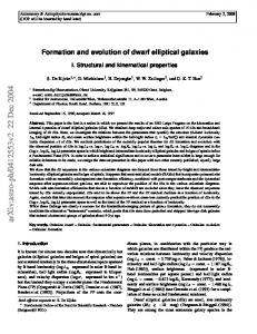
– 29 – Fig. 1.— The limits on the anisotropy radius for the consistency of the one–component γ models as a function of γ. The solid line represents the lower limit as determined by the NC, and the dotted line the upper limit as given by the WSC. For γ = (0, 1, 2, 3) the black dots connected by the dashed line represent the upper limits obtained using the SSC, while the true limits derived from the DFs are shown as black squares. The long–dashed line represents the limit on the anisotropy radius in presence of a dominant central BH. Fig. 2.— The dimensionless DF f1 /fN for the one–component γ = 1 model [solid line, Q(0) = Ψ1 (0) on the abscissae], and in the case of a dominant γ = 0 halo [limµ→∞ µ3/2 f1 /fN , Q(0) = Ψ0 (0) on the abscissae], when β = 0.2 (dotted line) and β = 3 (dashed line). In the upper panel the globally isotropic case is shown, while in the lower panel the anisotropy radius is fixed at ra = 0.26r1 . The −1/2 −3/2 r1 . normalization constant is fN = G−3/2 M1 Fig. 3.— The dimensionless DF f0 /fN for the one–component γ = 0 model [solid line, Q(0) = −1/2 −3/2 Ψ0 (0) on the abscissae, fN = G−3/2 M0 r0 ], and in the case of a dominant γ = 1 halo −1/2 −3/2 r1 ], when β = 0.2 (dotted [limµ→0 µ−1 f0 /fN , Q(0) = Ψ1 (0) on the abscissae, fN = G−3/2 M1 line) and β = 5 (dashed line). In the upper panel the globally isotropic case is shown, while in the lower panel the anisotropy radius is fixed at ra = 0.65r0 . Fig. 4.— The central value of the dimensionless isotropic [solid line, equation (36)] and anisotropic [dotted line, equation (37)] parts of the DF for the halo–dominated γ = 0 model, as a function of β = r0 /r1 , for β ≥ 1. Fig. 5.— The minimum value for the anisotropy radius of both components of (1,0) models in the case of a dominant halo, as a function of β = r0 /r1 . The anisotropy radius is normalized to the scale–length of the specific component. In panel (a) the solid line refers to the γ = 1 component, and the dotted line to the γ = 0 component. The two dashed lines represent the same quantities, when the halo mass is ten times the mass of the specific component. The black dots are the critical values of sa for the one–component models. Panel (b) is the enlargement of the small window at the top–right of panel (a). The dashed line shows the upper limit on sa due to the halo concentration effect.

(a)

(b)