barchan dunes that are used as a benchmark for our numerical model of
bedforms. ... selection and the evolution of a population of dunes over a wide
range of ...
River, Coastal and Estuarine Morphodynamics: RCEM 2005 – Parker & García (eds) © 2006 Taylor & Francis Group, London, ISBN 0 415 39270 5
Modelling of dune patterns by short range interactions Clément Narteau, Eric Lajeunesse, Franc˛ois Métivier & Olivier Rozier Equipe de Géomorphologie, Laboratoire de Dynamique des Systèmes Géologiques, Institut de Physique du Globe de Paris, Paris cedex, France
ABSTRACT: A 3D cellular automation is disclosed that enables modelling the dynamics of bedform. The overall mechanism can be regarded as a Markov chain, a discrete system with a finite number of configurations and probabilities of transition between them. Physical processes such as erosion, deposition and transport are modelled at the elementary scale by nearest neighbour interactions. At larger length scales, topographic structures arise from internal relationships based upon these short range interactions. This article focuses on crescentic barchan dunes that are used as a benchmark for our numerical model of bedforms. Length and time scales of isolated barchan dunes are studied in order to constrain the parameters of the model. Then we discuss pattern selection and the evolution of a population of dunes over a wide range of initial and boundary conditions. We eventually show that our model can be generalized to bedforms through the increase of the sand availability.
1
INTRODUCTION
There is a considerable variation within bedforms as they locally depend on the topography, the sediment load, and the flow. Such variability might be expressed by different relationships between erosion and deposition rates and the fluid velocity field. While empirical relationships estimate these quantities for a given bed under particular conditions, theoretical relationships simplify the turbulence problem to make easier the description of the sediment capacity of the flow. In both cases, it remains extremely difficult to tackle the impact of the size distribution of sediment particles. Despite these limitations, the study of aeolian dunes has significantly filled the gap between observations and models (Bagnold 1941; Pye and Tsoar 1990; Lancaster 1995). Under dry conditions, the transport of sand grains by the wind involves similar physical mechanisms than sediment transport in liquids. However the absence of cohesion, dissolution and sedimentation limits the number of relations between fluid and solid ingredients. Then, in order to investigate couplings between wind and topography, it is sufficient to formalize the wind velocity field with respect to the surface profile as well as the erosion and deposition responses to shear stress (Jackson and Hunt 1975; Hunt et al. 1988; Weng et al. 1991). In this framework, the principle of mass conservation is commonly ensured by a continuity equation for the height profile
where q is defined as a volumic sand flux per unit of time and per unit of length perpendicularly to the wind direction. The capacity of transport takes therefore the form of a saturated sand flux qs , and the only parameters are those which are relevant for the magnitude of qs according to the topography (Kroy et al. 2002a; Andreotti et al. 2002). Schematically, for a strong enough wind, deposition dominates if q approaches qs (i.e ∂x q < 0), else erosion occurs (i.e ∂x q > 0). In all cases, there are different ways the grains can be put into movement. First, they can be dragged, lifted and accelerated by the excess shear stress exerted by the fluid on the surface. This corresponds to saltation. Second, they can be released by impacts of falling grains and crawl on the surface. This corresponds to reptation. These two transport modes are obviously related to one another, essentially because saltation implies an irregular hopping process through the retroaction of transported grains on wind velocity. In this paper, we concentrate on the formation and the evolution of crescentic barchans dunes as a benchmark for a new model of sediment transport. Barchan dunes are isolated structures with horns extending downwind on both sides of an sand pile characterized by a slip face and a windward face (Fig. 1). Saltation and reptation are active on the windward face and the slope angle may vary from 10◦ to 15◦ ; the slip face is not submitted to the dominant wind and its geometry is controlled by avalanches of grains reaching the dune crest. The angle of repose of the sand being approximately of 30◦ , the dune profile is asymmetric in the direction of the wind. Barchans dunes have been observed in different geophysical environments
1035
2 THE MODEL Sediment transport is modelled by a Markov chain, a stochastic process characterized by a finite number of configurations evolving from one another according to a set of actions with different transition rates. 2.1
Figure 1. (a) Comparison between crescentic barchan dunes in air and water, in desert and laboratory experiments respectively (courtesy of Physical Review Letters, Hersen et al. (2002)). (b) Tranverse view of a barchan dune in Morocco (picture taken by B. Andreotti).
on Earth (arid desert, icecap, deep water), on Mars, but also in laboratory experiments (Fig. 1). They are propagating downwind, and independent relationships can be deduced from their dimensions, volumes and velocities. Overall, the aim of this paper is to compare the predictions of our model with these relationships. Following Nishimori and Ouchi (1993a) and Werner (1995), our numerical approach is dedicated to the analysis of emergence mechanisms in geomorphology. An emergence mechanism is met when one phenomenon leads to another, not in a direct cause/effect relationship, but in a manner that involves pattern of interactions between the elements of a system over time. In other words, an emergent macroscopic behavior can not be anticipated from the analysis of the constituent parts of the system alone, but can only result from their capacity to produce complex behaviours as a collective, through their mutual and repeated interactions. Such a complexity is an intrinsic property of cellular automata. Based on a discrete structure and a finite number of states at an elementary scale, cellular automata (CA) are systems that evolve on a network according to local interaction rules. These rules determine how each element responds to information transmitted from other elements along the network connections. Most of the time, these connections are simplified to include only interactions at a microscopic scale between nearest neighbors. CA are useful tools in physics, geophysics and biology to analyze pattern formation because their output match very well what we observe in nature without being dependent on a complete description of small scale processes. Thus, the origin of macroscopic behaviors as well as the emergence mechanism itself may be analyzed from a limited set of parameters. We exploit this property to implement a model conceptual enough to be applied on different types of geomorphological environments from aeolian dunes to river beds.
Length and time scales
A three-dimensional regular lattice models an interface between a turbulent fluid (air or water) and a layer of erodible sediment lying on a solid flat bedrock. This interface is subject to a so-called fluid action constant in magnitude and direction. An elementary cell has the shape of a parallelepiped, with 90◦ angles, a square base of length l and a height h. We focus on sediment flux rather than on individual particle motions and h is therefore equal to ld , the distance for a grain to accelerate up to the average fluid velocity:
where ρs , ρf and d are the grain density, the fluid density and the characteristic length scale of a grain respectively. The choice for such a length scale is motivated by observations in desert area and laboratory experiments (Bagnold 1941; Hersen et al. 2002) as well as by analytical results together with numerical simulations (Kroy et al. 2002b; Andreotti et al. 2002). The aspect ratio η = h/l corresponds to an upper limit of the slope angle θ upward in the direction of the flow (η = tan(θ) < 1). Finally, the characteristic time scale τ is determined from the dimensions of an elementary cell and an arbitrary volumic sediment flux Q (see Eq. 1):
2.2 The discrete dynamic Erosion does not affect the underlying solid bedrock and, at the bottom of the system, a layer of stable cells forms a flat surface where the transport of particles can create a topography. Then, we consider 4 states, 2 solid and 2 fluid. This is the minimum number of states necessary to implement retroaction mechanisms between a topography and a flow (Tab. 1). The two solid states, grains (G) and mobilized grains (M ), allow to implement the action of fluid shear velocity on the surface. The two fluid states, fluid (F) and excess shear stress (S), allow to implement the action of topography on the flow pattern. The indices (i, j, k), i ∈ [1, L], j ∈ [1, L], k ∈ [1, H ] label the Cartesian coordinates and the cell ci,j,k is either
1036
Table 1. 4 different states: 2 solid, 2 fluid. This is the minimum number of states to explore feedback mechanisms between circulation patterns and evolving topography. Action of fluid shear stress on topography
grains (G)
mobilized grains (M ) Action of topography on fluid motions
fluid (F)
Excess shear stress (S)
Figure 2. First neighbors in a regular rectangular parallelepiped mesh and the transition rates associated with a ci,j,k -cell. •
Grains (G): a G-cell represents a volume of sediment of uniform particle size. • Mobilized Grains (M ): a M -cell represents a volume of sediment transported by the fluid. Transportation of grains involves two transport modes related to one another: saltation and reptation. Here we do not differentiate between those modes. • Fluid (F): a F-cell represents a volume of fluid where the velocity is under a threshold of erosion. Furthermore, particles can not be transported and F-cells are agent of deposition. • Excess Shear Stress (S): a S-cell represents a volume of fluid where the shear stress exerted by the flow is above a threshold of erosion. S-cell are agent of erosion and transport by saltation and reptation. NG , NM , NF , NS are the number of G-cells, M -cells, F-cells, S-cells respectively, and
We do not consider long range interaction like other discrete approaches (Nishimori and Ouchi 1993b; Bishop et al. 2002), we only consider interactions between two neighboring cells with a common side (Von Neumann neighborhood, Fig. 2). These doublets
of neighboring cells are noted (ci,j,k , ci±1, j,k ), (ci, j,k , ci, j±1,k ) and (ci, j,k , ci, j,k±1 ). As detailed below, a cell may change states only if it shares an edge with a neighboring cell in a different state. In addition, we make a distinction between the orientation of the doublets according to gravity and the direction of the flow. This choice yields the lowest number of possible configurations and transitions while allowing for modelling of the physical processes involved in the formation of bedforms. The whole process is defined in terms of a Poisson process with stationary transition rates between the various possible states of the doublets of neighboring cells. Given a transition from state u to v, the probability distribution of the waiting time until the next transition is an exponential distribution with rate parameter λvu . Then the probability that a pair of neighboring cells in state u undergoes a transition toward the state v in the infinitesimal time interval dt is λvu dt. The practical way we proceed in the numerical simulations is detailed in appendix. The main point is that at each iteration three random numbers determine the time step, the doublet which undergoes a transition and the transition kind itself. Therefore the model possesses the Markov property as the next configuration (i.e. the future) is independent of the previous configurations (i.e. the past), given the knowledge of the present configuration. This probabilistic approach and the physical processes represented by different set of transitions distinguish our model from classical CA (Narteau et al. 2001). 2.3 The physical processes Each of the physical processes that we will now describe corresponds to a set of transitions. A transition of a given set cannot be considered in isolation because only combined and repeated actions are capable of reproducing these processes. For the same reason, transition rates are determined by reference to characteristic times representative of the given physical processes. 2.3.1 Fluid flow At a given altitude above a flat surface, the velocity field might be considered constant in magnitude and direction, and the velocity profile is known to increase according to a logarithmic function (Landau and Lifshitz 1963). This is not the case above a rough surface, over which a flow might produce an highly turbulent circulation especially when it involves erosion, deposition and transport. Here, we adopt simplifying assumptions to limit the scope of the model on fluid velocity above topography. As the streamlimes approach an obstacle, they converge and the velocity increases; after this obstacle, the streamlines diverge and the velocity decreases. Such observations are put into practical effect through the
1037
Practically, S-cells in contact with G-cells produce M cells upward and in the direction of the flow. These transitions are the only source of transport in the model. Taking the sediment flux Q as a control parameter, the magnitude of the transition rate λs is derived directly from τ (see Eq. 3).
Figure 3. Transition rates of the permutation between a S-cell located in ci, j,k and a F-cell located in ci±1, j,k , ci, j±1,k , ci, j,k±1 .
2.3.3 Transport If the fluid velocity is high, grains already in motion can be transported upward and in the direction of the flow. Such a transportation involves two transitions based on the permutation of M -cells in contact with S-cells:
motions of S-cells in an ocean of F-cell by considering the following transitions:
The magnitude of this sediment transport is proportional to Q and, by convention, the transition rates is taken equal to λs . 2.3.4 Deposition When the fluid velocity is not high enough to maintain particles in suspension, deposition occurs. This deposition of fluid-borne grains is enhanced by topographic obstacles and occurs faster on slopes of existing structures. This process involves the following transitions Each of these transition can be characterized by a vector according to the orientation of the doublet and the magnitude of the transition rate (Fig. 3). The resulting vector, i.e. the sum of the six vectors, determines the direction of the flow as well as the intensity of the turbulent diffusion. λw being an estimate of the turbulent j−1 j+1 diffusion, we take λw = λw = λwk−1 = λk+1 w = λw and λwi+1 > λw > λwi−1 . As a consequence, the flow is going eastward (Fig. 3). On the other hand, the velocity of this flow cannot be determined only by the transition properties, but, as explained below, it can be approached through the proportion of S-cells in the fluid.
where G-cells are created from M -cells if they are not in contact with S-cells. a > 1 and, for the sake of simplicity, we assume that the deposition rate is equal to λs , the erosion rate. 2.3.5 Diffusion Horizontal diffusion disperses the grains and flattens the topography. This process involve the following permutations between G-cells and F-cells:
2.3.2 Erosion Grains are lifted and dragged by the shear stress applied by the moving fluid and set in motions in the direction of the flow. This erosion process, which does not discriminate between saltation and reptation, involves two types of transition:
j−1
j+1
where λd = λdi−1 = λdi+1 = λd = λd a characteristic time for diffusion.
1038
is the inverse of
2.3.6 Gravity Sand grains fall under their own weight and exert pressure on all the other grains. Gravity prevents further motions and leads to deposition.We attribute the following transition to these gravitational processes:
Table 2. ld � Q λs τ λw τ λd τ λg τ a
Parameters of the model and their values. 0.44 m 11.3◦ 100 m2 ·yr −1 6 6 0.06 6000 10
They include downward permutations between G-cells and fluid-states as well as depositions of M -cells located under solid-states. λg is determined from the Stokes velocity and it is generally few orders of magnitude larger than all the other transition rates. 3
NUMERICAL SIMULATIONS
The model involves 20 transitions characterized by a limited number of independent transition rates. Before we present the results of the numerical simulations, different aspects of the model can be addressed when looking at all the transitions together. First, the conservation of mass is ensured by the constant number of solid cells (NG + NM = cte). Second, S-cells are persistent in all transitions (NS = cte) in such a way as to ensure the fluid forcing.As a consequence, we are dealing with an open system which relies on the balance between erosion and deposition to ensure the conservation of momentum at a macroscopic scale. For this reason, the proportion of S-cells in the fluid has to be low, β = NS /NF