Modelling of spatial-temporal changes of the geomagnetic field in Japan. Xiaoli Ji1, Mitsuru Utsugi2, Hiroki Shirai1, Akira Suzuki1, Jinlan He1, Satoshi Fujiwara1 ...
Earth Planets Space, 58, 757–763, 2006
Modelling of spatial-temporal changes of the geomagnetic field in Japan Xiaoli Ji1 , Mitsuru Utsugi2 , Hiroki Shirai1 , Akira Suzuki1 , Jinlan He1 , Satoshi Fujiwara1 , and Yoshihiro Fukuzaki1
2 Institute
1 Geographical Survey Institute, Kitasato-1, Tsukuba, Ibaraki 305-0811, Japan for Geothermal Sciences, Graduate School of Science, Kyoto University, Kawayo, Minami-Aso, Kumamoto 869-1404, Japan
(Received April 28, 2005; Revised August 9, 2005; Accepted August 16, 2005; Online published June 2, 2006)
A geomagnetic regional model is constructed to provide a spatial-temporal variation of three orthogonal components (X, Y, Z ) in Japan. In order to obtain a high temporal and spatial resolution, Natural Orthogonal Components (NOC) analysis and Spherical Cap Harmonic (SCH) analysis were employed to produce a spatialtemporal model based on the observed data from geomagnetic observatories and continuous geomagnetic stations. Using this model, we calculated the secular variation between 1999 and 2004 in Japan. The root mean square (RMS) scatter of the model is less than 3 nT, which indicates a good agreement between calculated and input data. Key words: Geomagnetic regional model, spatial-temporal model, secular variation, Natural Orthogonal Components, Spherical Cap Harmonic.
1.
Introduction
The main geomagnetic field changes both spatially and temporally. In order to investigate the spatial distribution of the main field in Japan, the Geographical Survey Institute (GSI) carried out the measurements at first- and secondorder geomagnetic stations. Three components (horizontal intensity (H ), declination (D), vertical intensity (Z )) and total intensity (F) are measured at these stations and the obtained data are used to produce magnetic charts of Japan which are published every ten years. The latest charts, epoch 2000.0, are now available (Shirai et al., 2002). The magnetic charts provide accurate geomagnetic field values for Japan and are widely used as a reference for the study of local geomagnetic anomalies in this region. However, they give no detailed information about the secular variation since the charts are produced every ten years (tenyear resolution) only. On the other hand, main field and secular variation can be obtained with spatial-temporal models such as the International Geomagnetic Reference Field (IGRF). However, IGRF models the main field to a minimum wavelength of 1500 km and the secular variation to 2000 km. Therefore, it is difficult for IGRF to yield a detailed description of the geomagnetic field and its change over Japan. In order to obtain a precise model, we develop a regional secular variation model. The accuracy of the model depends on the analytical method and the quality of data. In this study, Natural Orthogonal Components (NOC) and Spherical Cap Harmonic (SCH) techniques are chosen to construct a model based on the observed data from 5 geomagnetic observatories and 9 continuous geomagnetic stations. The data from the firstand second-order geomagnetic stations, where the measurec The Society of Geomagnetism and Earth, Planetary and Space SciCopyright � ences (SGEPSS); The Seismological Society of Japan; The Volcanological Society of Japan; The Geodetic Society of Japan; The Japanese Society for Planetary Sciences; TERRAPUB.
ments are not performed continuously, are not selected because the NOC technique requires continuous data series over the whole time interval. Although the total amount of data used for the modelling is not large, such data has been successfully used to construct a spatial-temporal model of the geomagnetic field in Japan (Fujiwara et al., 2001). We consider these data sufficient to establish a regional model for the study of the secular variation. The main aim of this work is to describe the construction and the evaluation of the model. The details of the modelling methods and data will be introduced first.
2.
Modelling Method
To obtain a spatial-temporal model with high temporal and spatial resolution, we chose NOC (Langel, 1987; Burdelnaya et al., 1999) and SCH techniques (Haines, 1985). The principles of these techniques are described below. Since the main field changes both spatially and temporally, the time series of a field component at location p, M p(t), can be expressed as M p (t) =
L �
X p,l · Tl (t) + δ p (t),
(1)
l=1
where l represents the number of certain combinations of temporal function Tl (t) and spatial function X p,l , δ p (t) is random error. Because the observed field in Japan exhibits similar temporal behavior, the solution of Eq. (1) can be derived by NOC analysis which provides a mean of reducing the number of principal temporal functions (T1 (t), T2 (t), . . . , TL (t)). These temporal functions reflect common changes of the field and satisfy the following orthogonality conditions. � � �= 0 (k = l) Tk (ti ) · Tl (ti ) (2) = 0 (k �= l), i
757
758
X. JI et al.: MODELLING OF THE GEOMAGNETIC FIELD IN JAPAN
leads to the construction of an orthogonal, complete set of basis functions. Haines (1989) advocated the mixing up of MMB the two sets, although they are not orthogonal to each other, AKA to achieve uniform convergence. The coefficients gkm and h m k are determined by the least YOK squares method. The orthogonal components (X, Y, Z ) of MIZ the observed field in geodetic coordinate are transformed to HAR SIK a cap coordinate and are derived by computing the approHAG KAK 35 oN priate spatial derivatives of the potential V with coefficients YOS KNZ gkm and h m k . TTK To construct the secular variation model, our data conKUJ sisted of the field variation with respect to a reference epoch KNY for both the NOC and SCH analyses. The epoch of 2000.0 was chosen to be the reference year in this study. In the spatial analysis, X , Y and Z , which were the changes OKI in the three components at epoch t relative to the values at 25 oN 125 oE epoch 2000.0, were derived from the corresponding poteno 145 E 135 oE tial change V using Eqs. (1) in An (2003).
F, D and H denoting the changes in total intensity, Fig. 1. Location of the magnetic observatories (solid triangle) and contin- declination and horizontal intensity at epoch t relative to uous geomagnetic stations (solid circle) used in the regional model. epoch 2000.0, respectively, were then calculated from X ,
Y and Z , assuming that the changes of the field were within the range of the first-order linear approximation. Tl (t) are arranged in decreasing order of power contain. When the most powerful temporal functions are selected, 3. Description of the Data Set the observed field M p (t) can be fitted with small residuals. The geomagnetic data were provided by GSI and the Since M p (t) is expressed in nT, we relate this unit to the Japan Meteorological Agency (JMA). The distribution of spatial function X p,l . the sites is shown in Fig. 1. There are two types of sites: 5 NOC analysis allows us to calculate the field components geomagnetic observatories at Memambetsu (MMB), Mizuonly at location p. In order to compute the field at an arbi- sawa (MIZ), Kakioka (KAK), Kanozan (KNZ) and Kanoya trary position in the region, a spatial model is required. In (KNY), and 9 continuous geomagnetic stations (continuthis study, the SCH technique was chosen. The SCH mod- ous stations) at Akaigawa (AKA), Yokohama (YOK), Haraelling is devoted to potential and field representation in a machi (HAR), Shika (SIK), Hagiwara (HAG), Yoshiwa spherical cap. Although the method poses many difficulties (YOS), Totsukawa (TTK), Kuju (KUJ) and Okinawa (OKI). (Hwang and Chen, 1997; Thebault et al., 2004), it has been At the continuous stations, H, D, Z and F are measured with widely employed in deriving regional geomagnetic models, fluxgate and proton magnetometers. They are operated fully for example, for Canada, Africa and China regions (Haines, automatically and the data is transmitted to GSI through the 1985; Kotze, 2003; An, 2003). public telephone line. The fluxgate magnetometer data is In a spherical cap area, the potential of the internal field sampled every minute and absolute observation is carried is expanded as follows: out once a year for the baseline determination. Although the 45 oN
K max � k �
a · (a/r )n k (m)+1 · (gkm · cos mφ + h m k · sin mφ)
k=0 m=0 · Pnmk (m) (cos θ ),
(3)
where a is the mean radius of the earth, (r , θ, φ) are the geocentric spherical coordinates of radius, colatitude and longitude, respectively, with respect to the axis of the cone; gkm m and h m k are the Gauss coefficients. Pn k (m) is the associated Legendre function with m and nonintegral degree n k (m). n k (m) is the root of the following equations d Pnmk (m) (cos θ0 )/dθ = 0 (k − m = even) or Pnmk (m) (cos θ0 ) = 0 (k − m = odd) ,
29830
(4)
X (nT)
V =
29790
29750 1999
2001
2003
2005
where θ0 is the aperture of the spherical cap. These equaYear tions correspond to one of the boundary condition of two Sturm-Liouville problems. The second boundary condition, Fig. 2. Temporal variation of three-month means and fitting between 1999 solution finite at θ = 0, ruling out the Legendre functions and 2004 for the X component at Kakioka (KAK). of the second kind. Each of the Sturm-Liouville problems
X. JI et al.: MODELLING OF THE GEOMAGNETIC FIELD IN JAPAN
30
26520
Table 1. Multivariate regression results for the X component at Akaigawa (AKA).
0
Parameter
Estimated values
P-value
M0
26484 0.725 0.216 1.074