conductive and capacitive coupling. When a power transmission line runs in parallel with a pipeline for a considerable length, induced AC voltages may appear ...
Australasian Universities Power Engineering Conference (AUPEC 2004) 26-29 September 2004, Brisbane, Australia
MODELLING OF THE INTERACTION BETWEEN GAS PIPELINES AND POWER TRANSMISSION LINES IN SHARED CORRIDORS D.Markovic, V.Smith, S.Perera, S.Elphick School of Electrical, Computer and Telecommunications Engineering University of Wollongong, NSW 2522 Australia Abstract Sharing of common corridors by gas pipelines and overhead power transmission lines is becoming quite common. Voltages can be induced on gas pipelines from power transmission lines in the sections where they share the corridor. This paper reports on a recently completed study on the interaction between gas pipelines and power transmission lines in a utility common corridor in New South Wales, Australia. A previously developed computer program was used to perform a detailed analysis of the induced voltages and pipeline potentials during steady state and fault conditions. Mitigation measures are proposed to ensure compliance with standards that regulate this area. 1.
potential difference. This potential may cause coating damage or if the conductive fault current is sufficiently large, a direct arc between a tower leg and a buried pipeline may be initiated resulting in a pipeline puncture [1, 2].
INTRODUCTION
While there are significant benefits in sharing a corridor between pipelines and power transmission lines, e.g. joint land use, there are also many concerns. The main ones are: • Safety considerations for operation and maintenance personnel on pipelines • Direct effects on the pipeline, e.g. corrosion, coating damage or even puncture • Effects on the electrical or electronic devices used for cathodic protection, metering, monitoring and other type of equipment associated with the pipeline
Many studies have been produced dealing with induced voltages, but only few have field measurement results that can be compared with the computed results [3-5]. 2.
OBJECTIVE
The objective of this study is to improve understanding of several computer modelling issues regarding the length of the pipeline model, and to confirm the accuracy of steady state induced AC voltage prediction methods by comparing results from the software analysis with measured data. A quantitative parametric analysis of induced AC voltages on a 42 km long section of gas pipeline in New South Wales was undertaken. This analysis aimed to identify any important problems resulting from induced AC voltages on the pipeline and to suggest an additional mitigation strategy to those currently existing on the pipeline.
Electrical energy can be transferred from power transmission lines to pipelines through inductive, conductive and capacitive coupling. When a power transmission line runs in parallel with a pipeline for a considerable length, induced AC voltages may appear on the pipeline. The magnetic field of a power transmission line is mostly dependent on the currents in its conductors, which in turn is the main factor in determining the induced voltage on the pipeline. Some of the other factors that can increase induced AC voltages on the pipeline are length of exposure between the power transmission line and the pipeline, phase sequence of conductors, distance between the power transmission line and the pipeline and soil resistivity. Inductive coupling is the only coupling that occurs during the normal load condition, and it rarely imposes excessive stress on the pipeline.
3.
COMPUTER MODELLING
Shared corridors between power transmission lines and pipelines are becoming more complex. Inside the corridor, pipelines and power lines usually never run exactly parallel to each other. There are often frequent changes of the angle between them, changes of the distance between them, or the pipeline changes the side which it runs along the power transmission line. Often data about the physical position of the pipeline relative to the power transmission line is not available or is incomplete. The longer the examined corridor, the more complex the handling of all these minor
Conductive coupling occurs in the case of a single phase to earth fault on the power transmission line. The fault current will flow through a tower into the earth. The potential of the ground will rise and the coating of the pipeline will be subjected to a high
1
commercially available programs. The major limitation is that multi layered soil can not be modelled. The software treats soil resistance as being vertically uniform. This can introduce an error of up to the magnitude of the calculated value of the pipeline potential in a fault study.
changes becomes. For the above reasons it is often necessary to resort to approximations. The common corridor can be divided into several simple sections, each of which represents a part of a real common corridor with similar features. For instance if a pipeline runs along the power transmission line at an angle of 5 degrees, the corridor can be modelled as if the pipeline and power line are parallel.
4.2
The software uses the following procedure for calculation of induced voltages on a pipeline [6]: 1. From the interaction geometry determine the appropriate distances and locations of the active and passive conductors 2. Using Carson’s equation or its alternative determine the LEF (longitudinal electric field) driving the pipeline along its complete length. 3. From the pipeline electrical and physical parameters determine its propagation constant and characteristic impedance. 4. Develop a pipeline circuit model and solve for the induced voltage and current levels.
Fault analysis requires more precision in dividing the shared corridor into sections than steady state analysis. The fault current goes into the earth through a tower to the soil, and pipeline potentials will be very dependent on the tower position in the computer model. The computer model assumes that each modelled section ends with a tower, so extra consideration should be given when deciding how long each section of a model will be. Proper division of a power transmission line and pipeline common corridor into sections requires considerable modelling experience. 4.
SOFTWARE
4.1
Software Description
In addition to inductive coupling, resistive (conductive) coupling through the earth must be considered while determining fault coupling levels. The methodology for this was taken from Sobral [7].
Calculations in this study have been performed using a software package that came with a report by Dabkowski [6]. This software package was prepared for PRC International at the AGA (American Gas Association) with a goal of creating an extremely user friendly interface that will allow member companies to undertake their own inductively coupled interference studies. It is not a commercial program and it has certain limitations in comparison with pipeline power transmission line
Induced Voltage Calculations
5.
CASE STUDY
The analysis and field measurements in this project were performed on an existing pipeline and power transmission line shared corridor in New South Wales, Australia and is described below.
Line 2 (132 kV)
Line 1 (132 kV) Line 5 (66 kV) Line 3 (66 kV)
Line 6 (132 kV)
Line 4 (132 kV) 170
180
186
194
insulating joint 204
Distance in km
Fig. 1 Physical layout (not to scale) of the shared corridor
2
208
212
resistivities were obtained by interpolating known soil resistivities in the neighbouring areas.
power transmission line pipeline Line 5 (66 kV)
5.3
All five power transmission lines that run through the common corridor have horizontal wooden towers. They consist of one three phase electrical circuit and two shield wires. Line 1 in Figure 1 is transposed several times over its entire length. The steady state calculations were made with the assumption that the load currents are balanced. The steady state induced voltages are sensitive to current unbalance. The fault current by itself is an unbalanced case (phase to earth fault) and the load current unbalances are negligible during the fault (if they exist). The current logs for Line 1 show that the minimum current was 265 A and the maximum was 325 A. Calculations were done with 300 A as that was the approximate loading at the time of the measurements. Line 6 has a maximum designed rating of 440 A, and that current, even though giving conservative results, was used in the study. The current in Line 4 was 440 A and the current in Line 2 was 200 A. Currents in both 66 kV Lines, 3 and 6 were 100 A. The currents in Lines 5 and 4, and the currents in Lines 3 and 6 were the same because of a limitation of the software to accept more than five power transmission lines in a single study. There are six lines in the shared corridor and two lines were needed to model conductor transposition on Line 1.
Line 6 (132 kV) insulating joint
208
212 Distance in km
Fig. 2 Section 208-212 5.1
Shared Corridor
The pipeline under study (Fig.1) is 212 km long and kilometre markers are used throughout the study to mark distance along the pipeline. Insulating joints are used to electrically separate sections of the pipeline from terminal facilities and pumping systems. In the case of development of contact with other structures or the failure of cathodic protection units these problems are confined within a single section. In our case study insulating joints are located at the end of the pipeline at point 212 and at point 120. The corridor, where the pipeline runs parallel to a number of power transmission lines, exist between points 170 and 212 and only this 42 km segment will be part of this study. In analysing this segment of the pipeline, three sections were identified as being in a high risk zone for induced AC voltages from nearby power transmission lines. Those sections were 170-186, 194204 and 208-212. In the section 170-186 the pipeline shares the corridor with a 132 kV power transmission line (Line 1). The next section, 194-204, is the most complex since four different power transmission lines run in parallel with the pipeline. Three of the power lines are 132 kV (Lines 1, 2 and 4) and the fourth one is 66 kV (Line 3). The section 208-212 has two power transmission lines running in parallel with the pipeline, one at 132 kV (Line 6) and the other at 66 kV (Line 5). This section is shown in Fig.2. 5.2
Power transmission line
5.4
Short and long pipeline models
The main objective of this study was to develop computer models of the shared corridor that can accurately predict induced AC voltages on the pipeline. Secondary to this was an aim to determine whether or not accurate voltage predictions at a certain point on the pipeline can be obtained by modelling just a small critical section around the point or if it is necessary to model all other existing critical sections in the proximity of that point, which is a very complex task. To fulfil these objectives two computer models have been developed.
Pipeline and soil resistivity
The first model (long model) includes the entire 42 km section as it appears in Fig. 1. The second model (short model) only includes the critical part of the pipeline between 207 and 212 as shown in Fig. 2. Results from both models are compared with field measurements and with each other.
Data was obtained from the gas utility that owns the pipeline under study. The pipeline is steel with 168.3 mm outer diameter and 4.8 mm wall thickness. Applied coating on the pipeline is high density polyethylene known as yellow jacket. 32 testing points (where voltages and currents can be measured) exist along the 42 km length of the pipeline. Structure of the ground in the studied section is not constant and soil resistivity of the top layer is in the range of 5500 to 37000 ohm-cm. Multilayer soil resistivities for several points of the corridor were obtained from a Pipeline Authority report [8], but for many other sections there was no available data. For the areas of shared corridor where there was no data available, soil
6.
RESULTS
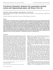
6.1 Comparison of calculated steady state voltages and field measurements The calculated steady state AC voltages on the pipeline in the shared corridor were compared with the induced AC voltages (measured with digital voltmeter and a reference cell at the test points in the field) and
3
20
Induced Voltage (V)
Measured Calculated
15
10
5 Distance km
17 0. 17 5 2. 17 3 3. 17 6 5. 17 5 6. 17 5 8. 18 1 0. 1 18 2. 18 2 3. 18 9 5. 18 3 6. 18 9 8. 19 8 0. 19 5 2. 3 19 4. 19 2 5. 19 8 7. 19 5 9. 20 5 0. 8 20 20 2 3. 20 5 3. 6 20 4. 20 2 5. 20 8 7. 20 4 8. 9 20 9 20 9. 9 21 2
0
Fig. 3 Comparison between calculated and measured induced voltages on the pipeline parallel) can not be considered correct if there are other similar critical sections further along the pipeline. Calculations completed together with these additional sections can sometimes introduce higher calculated induced voltages in the viewed section. Analysis of just one critical section of a common corridor, disregarding the other common parts of the corridor further along the pipeline should only be attempted when data and physical features of the other parts of the corridor are not known. In that case results should be taken only as an estimate.
the results are shown in Fig. 3. One of the limiting factors in this comparison between the calculated values and the measured values is the time that it takes to complete measurement on all of the test points along the pipeline. This may require one or two days of field measurements. During that time currents in power transmission lines change according to their daily loading cycle, which cause changes in induced AC voltages on the pipeline. This fact can cause some mismatching during comparison of all measured points at the same time. Modelling of the pipeline was done with 4Ω earthing at points 170 and 212 to match the actual earthing status of the pipeline.
Further analysis observed the influence of the combination of the phase sequence of the two power transmission lines in the common corridor on induced voltages on the pipeline. Comparisons between the short and long models were made again (Fig.4, where RWB stands for marking phase sequence: red, white and blue). According to theory the highest induced voltages occurred when the phase sequences in both power transmission lines were the same (three most right bars at point 208 and 212 in Fig. 4). But when the whole 42 km of common corridor was taken into account in the modelling, the highest induced voltage on the pipeline at point 212 was when phase sequences in the power transmission lines were different (three most left bars at point 212 in Fig. 4).
From Fig. 3 it can be seen that the peak value measured at point 180.1 aligns well with the simulated result. If we analyse the graph we can conclude that the matching of measured and calculated values is better in the first half of the corridor. That area is simpler, consisting of one pipeline and one power transmission line. Once we come across more complexity in the second half, the departure of calculated values from measured ones become more obvious. But the important aspect is that peak induced AC voltages and their position along the pipeline were predicted reasonably. These values were compared with the relevant Standard [9] and mitigation measures were designed according to the position of the induced peak voltage along the pipeline (see Section 7).
20 18 16 Induced Voltage (V)
6.2 Comparison between short and long models The calculated steady state induced AC voltages on pipeline at points 208 and 212 were obtained using the long (Fig.1) and the short (Fig 2) models. The voltages in the first case were considerably higher than in the second case. This suggests that the steady state results obtained within one critical section (short model, where the pipeline and power transmission line run in
14 12
RWB - RWB RWB - WBR RWB - BRW RWB - RWB RWB - WBR RWB - BRW
10 8 6 4 2 0 170
176.5
178.1
180.1 203.5 Distnce km
204.2
208
Fig. 4 Effect of phase sequence
4
212
This again suggests that existence of additional critical sections further along the pipeline can have considerable influence on the viewed section. It should be noted that the power transmission line currents used in this part of the study were default values given by the computer program. Actual currents are higher, and the induced currents on the pipeline in this case are slightly less than measured values. 6.3
pipeline and the second and the fourth come from modelling only the last 4 km (short model) of the pipeline. A similar comparison was then repeated for the case where 4 ohms grounding was placed at the end of pipeline at point 212. Again the first and the third bar come from modelling 42 km (long model) of the pipeline and the second and the fourth bar come from modelling only the last 4km (short model) of the pipeline. This time the conclusion that higher pipeline potentials are obtained when 42 km of the pipeline is modelled can not be drawn. It appears to be correct for several points along the critical section 208-212 but as the fault is modelled closer to the end of the pipeline this is no longer the case. As expected the pipeline potentials are higher in the case when the pipeline was modelled non earthed. The values in Fig. 6 (when the pipeline was earthed) are still higher than the values allowed by the Standard [9]. For this type of pipeline (classified as pipeline with limited public access), the allowed pipeline potential during the fault is 1000 V. The pipeline was built and the original design was made when a previous version of the Standard [9] was applicable. According to the previous version of the Standard, during a fault on the power transmission line, a pipeline potential of 1500 V was allowed. This is a possible explanation as to why the fault levels are higher than allowed by the current Standard.
Pipeline potential due to power line faults
During a fault on the power transmission line on top of the inductive component of the induced AC voltage there is an additional conductive component. It has been shown in [7] that both the inductive and the conductive component could be classified by the strength of the longitudinal electric field. Regarding the pipeline potential both of these components are of the same phase and they are additive. The computer program used in the study recognizes this fact and the output of the program is the pipeline potential originating from both the inductive and the conductive component. Since this pipeline potential is location dependent, obtaining representative fault analysis of the pipeline requires consideration of the fault at many towers. Maximum Fault Voltage (V)
3500 3000 2500
42 km no IJ 4 km no IJ 42 km with IJ 4 km with IJ
2000
The software used in the study has a limitation with calculating the fault state pipeline potential because it can only treat soil resistivities as uniform. In the worst case inability to model multi layered soils can cause an error of up to the magnitude of the calculated fault state pipeline potential.
1500 1000 500 0 209.9
210.4
210.7 211 211.4 Fault at Distance (km)
211.7
212
Fig. 5 Non earthed pipeline potential during fault
2500
Maximum Fault Voltage (V)
The fault analysis was performed in a similar fashion as the steady state analysis. The fault current level of 11000 A was taken from report [8] and it comes from the power utility. The critical section between points 208 and 212 was modelled separately from the rest of the pipeline (short model). Then the entire section between points 170 and 212 was modelled in one file (long model) and the results were analysed. The comparisons were made in two cases: when the critical section was not earthed (Fig.5) and when the critical section was earthed (Fig.6). The latter is the case on the actual pipeline. For each case the pipeline was modelled terminating with the IJ (insulating joint) and not terminating with the IJ. As in the case with the steady state analysis, the values of the pipeline potential during the fault were higher in the case when whole 42 km (long model) of the pipeline was modelled than they were in the case when only 4 km (short model) critical section was modelled. In Fig. 5 the first and the third bar (looking from left to right) come from modelling 42 km (long model) of the
42 km no IJ 4 km no IJ 42 km with IJ 4 km with IJ
2000
1500
1000
500
0 209.9
210.4
210.7 211 211.4 Fault at Distance (km)
211.7
212
Fig. 6 Earthed (4Ω) pipeline potential during fault In any case the values obtained indicate that the potentials on the pipeline during faults are higher than allowed by the Standard [9]. Even if program limitations are taken into account, the calculated pipeline potentials during a fault are still too high. Therefore, it is recommended that the pipeline owners conduct a more detailed study featuring multilayered soil resistivities. This type of a study can finally reveal whether there is a need for additional fault state mitigation or not.
5
7.
corridor. It was shown that in the case of very complex shared corridors, steady state and fault state modelling of just one critical part of the pipeline without taking into account other critical parts along the pipeline would yield induced voltages of a lower magnitude than those obtained when all critical sections were analysed together. It was also shown that the worst case induced voltage for the same phase sequences on two power transmission lines in separately analysed short shared corridor sections, might not be the worst case when other critical sections along the pipeline are taken into account. The accuracy of computer modelling was confirmed by comparing the calculated steady state AC induced voltages with the field measurements. These comparisons showed good correlation.
PIPELINE POTENTIAL MITIGATION
Methods for mitigating the pipeline potential in the design stage are: avoiding longer parallel running of the pipeline and the power transmission lines, increasing the distance between the pipeline and the power transmission line as much as possible or the installation of shield wires on the power transmission line if they do not already exist. Once the pipeline is built, different approaches to pipeline potential mitigation apply. The simplest measure is a plain ground bed at a single location which will earth the pipeline. This method is usually convenient in the case when there is a single separated induced voltage peak. Where several induced voltage peaks are located close to each other, a single ground bed will not be sufficient. In this case voltage peaks can be mitigated with distributed ground anodes, cancellation or gradient wires. Distributed ground anodes can be vertical or horizontal and their number and the position on the pipeline where they need to be applied are determined by calculations. Alternatively, a cancellation wire may be installed. A cancellation wire is a wire placed along the pipeline such that its coupling with the pipeline cancels the induced voltages. It is not very popular today because it can introduce high potentials at its ends. The most popular and most effective way of mitigating induced voltages on pipelines is a gradient wire. A gradient wire is a wire that is placed in the ground next to the pipeline and it is connected to the pipeline at certain intervals.
9.
[1] Y.Li, F.Dawalibi, “Electromagnetic Interference Caused by a Power System Network on a Neighbouring Pipeline” International Symposium on Electromagnetic compatibility, Beijing, May 21-23 1997, pp 215-218 [2] F.Dawalibi, A.Pinho “Computerized Analysis of Power Systems and Pipelines Proximity Effects” IEEE Transactions on Power Delivery Vol PWRD-1 No.2, April 1986 pp40-48 [3] A.Taflove, J.Dabkowski “Prediction Method for Buried Pipeline Voltages due to 60 Hz AC inductive coupling Part I – Analysis” IEEE Trans. On Power Apparatus and Systems Vol. PAS-98, No.3, May/June 1979, pp 780-787 [4] A.Taflove, J.Dabkowski “Prediction Method for Buried Pipeline Voltages due to 60 Hz AC inductive coupling Part I – Field Test Verification” IEEE Trans. On Power Apparatus and Systems Vol. PAS-98, No.3, May/June 1979, pp 788-794 [5] A.Taflove, J.Dabkowski “Mutual Design Considerations for Overhead AC Transmission Lines and Gas Transmission Pipelines” Final Report EPRI EL-904, AGA Cat No. L51278, IIT Research Institute, Chicago, IL Sept 1978 [6] J.Dabkowski “AC Predictive and Mitigation Techniques” Final Report PR-200-9414, Crystal Lake, IL, Oct 1998 [7] S.T.Sobral “Interferences Between Faulted Power Circuits and Communication Circuits of Pipelines – Simplification Using the Decoupled Method” IEEE Trans. On Power Delivery, Vol.9, No.3, July 1994, pp1593-1599 [8] The Pipeline Authority “Moomba to Sydney Natural Gas Pipeline – Final Design Report for Induced Voltages” Williams Brothers – CMPS Engineers, 1986 [9] AS/NZS 4853:2000 “Electrical hazards on metallic pipelines”.
In the case of steady state analysis of the pipeline in this study, there is only one separate single voltage peak (20 V at point 180) that exceeds the value allowed by the Standard [9] (15V). Modelling shows that this voltage can be mitigated by applying a 4 ohm single ground bed at point 180. However, this ground bed created a so called “balloon effect”. After mitigating the voltage peak at point 180, another induced voltage peak at point 190 was introduced. Further modelling showed that an additional single ground bed with resistance of 10 ohms applied at point 190, successfully mitigated both voltage peaks The above proposed steady state mitigation must be compliant with the fault state mitigation requirements that have not been investigated. Once the precise fault state analysis is completed, the final mitigation measures can be proposed. These measures must satisfy both the steady state and fault state mitigation requirements. 8.
REFERENCES
CONCLUSIONS
Several aspects of computer modelling of gas pipelines for induced voltage were analysed using an existing pipeline and power transmission line shared
6