Passenger Demand using Computer-based Stated Preference Surveys, ...... error component of the utility can also be considered independent of ..... (Hague Consulting Group 1992) are generally implied for estimating logit models, mostly due ...
MODELLING PASSENGER MODE CHOICE BEHAVIOUR USING COMPUTER AIDED STATED PREFERENCE DATA
Omer Khan
BE (Mathematical Modelling)
School of Urban Development Queensland University of Technology Doctors of Philosophy (IF49) July, 2007
Abstract
Redland Shire Council (RSC) has recently completed the preparation of Integrated Local Transport Plan (ILTP) and started its implementation and monitoring program. One of the major thrusts of the ILTP is to reduce the car dependency in the Shire and increase the shares of sustainable environmental-friendly travelling modes, such as walking, cycling and public transport.
To achieve these objectives, a mathematical model is needed that is capable of modelling and forecasting the travelling mode choice behaviour in the multi modal environment of Redland Shire. Further, the model can be employed in testing the elasticity of various level-of-service attributes, under a virtual travel environment, as proposed in the ILTP, and estimating the demand for the new travelling alternatives to private car, namely the bus on busway, walking on walkway and cycling on cycleway.
The research estimated various nested logit models for different trip lengths and trip purposes, using the data from a stated preference (SP) survey conducted in the Shire. A unique computer assisted personal interviewing (CAPI) instrument was designed, using both the motorised (bus on busway) and non-motorised travelling modes (walking on walkway and cycling on cycleway) in the SP choice set. Additionally, a unique set of access modes for bus on busway was also generated, containing hypothetical modes, such as secure park and ride facilities and kiss and ride drop-off zones at the busway stations, walkway and cycleway facilities to access the busway stations and a frequent and integrated feeder bus network within the Shire. Hence, this study created a totally new virtual travel environment for the population of Redland Shire, in order to record their perceived observations under these scenarios and develop the mode choice models.
From the final model estimation results, it was found that the travel behaviour forecasted for regional trip-makers is considerably different from that of local tripmakers. The regional travellers for work, for instance, were found not to perceive the
i
non-motorised modes as valid alternatives to car, possibly due to longer trip lengths. The value of time (VoT) determined for local work trip-makers (16.50 A$/hr) was also found to be higher than that of regional work trip-makers (11.70 A$/hr).
From the survey analysis, a big part of the targeted population was found to be car captives, who are not likely to switch from cars to public transport; even if a more efficient transit infrastructure is implemented. In the past, the models have been generally calibrated using the mode choice survey data only, while that of the captive users were ignored. This yields a knowledge gap in capturing the complete travel behaviour of a region, since the question of what particular biases can be involved with each model estimation parameter by the captives remain unresolved. In this research, various statistical analyses were performed on the car captive users' data by categorising them into various trip characteristics and household parameters, in order to infer the relative influence of the car captive population on the travel behaviour of the study area.
The outcomes of the research can assist the policy makers in solving the strategic issues of transit planning, including the future development of a busway corridor, with an efficient transit access mode network. The research findings can also be utilised in evaluating the feasibility of developing walkways and cycleways in the Shire, along with appraising the relative influence of car captive users on the travel behaviour forecasts for the study area.
-----------------------------------------------------------------------------------------------------Keywords:
mode choice modelling; stated preference survey; CAPI; captive analysis; busway; walkway; cycleway; access modes. ii
Statement of Original Authorship The work contained in this thesis has not been previously submitted to meet requirements for an award at this or any other higher education institution. To the best of my knowledge and belief, the thesis contains no material previously published or written by another person except where due reference is made.
Omer Khan
Date:
/ /
iii
Acknowledgements
I wish to express profound gratitude to my principal supervisor Prof. Luis Ferreira and my associate supervisor Dr. Jonathan Bunker for their thoughtful guidance and constructive support in conducting this research. I also wish to thank Dr. Partha Parajuli (Transport Advisor, Redland Shire Council) for his professional advice during the preliminary and implementation phases of the study. Moreover, I would like to acknowledge the Faculty of Built Environment and Engineering, QUT and Redland Shire Council for providing financial support during my candidature.
I would like to express special appreciation to Mrs. Clara Tetther, Mr. Bradley Jackson and Mr. Nasir Ahmad for conducting the travel surveys, as part of this study, and for their assistance in the sample generation process. Finally, I would like to thank my family, fellow researchers and friends for their consistent encouragement during the research.
iv
Dedication
I wish to dedicate this PhD thesis to my grand-mother, Saeeda Ansari, my father, Ishtiaq Ahmed Khan, and my mother, Shubnam Ishtiaq, for their unlimited prayers, love and support, and to my brother, Osama, and two sisters, Nadia and Hinozia, for their consistent appreciation and moral support, and to my two beautiful nieces, Aliza and Eshal.
v
List of Abbreviations
•
ILTP
Integrated Local Transport Plan
•
IRTP
Integrated Regional Transport Plan
•
RSTS
Redland Shire Transportation Study
•
SP
Stated Preference
•
RP
Revealed Preference
•
VoT
Value of Time
•
O-D Matrix
Origin-Destination Matrix
•
IIA
Independence of Irrelevant Alternatives
•
CAPI
Computer Assisted Personal Interviewing
•
PAPI
Paper-and-Pencil based Interviewing
vi
Publications from this Research
•
Khan, O., Ferreira, L., Bunker, J. and Parajuli, P. (2007). High speed bus-onbusway market projections: stated preference survey design and mode choice modelling, Transportation Research Record, (In Press).
•
Khan, O., Ferreira, L., Bunker, J. and Parajuli, P. (2007). Modelling Multimodal Passenger
Demand
using
Computer-based
Stated
Preference
Surveys,
Australasian Transport Research Forum (ATRF) 2007, (Paper submitted). •
Khan, O., Ferreira, L., Bunker, J. and Parajuli, P. (2005). Design of a computer based survey instrument for modelling multimodal passenger demand. 27th Conference of the Australian Institutes of Transport Research, Brisbane, Australia.
•
Khan, O., Ferreira, L. and Bunker, J. (2004). Modelling multimodal passenger choices with stated preference data. 26th Conference of the Australian Institutes of Transport Research, Melbourne, Australia.
•
Conducted a session on "Mode Choice Modelling" in a 3-day short course on “Modelling in Transport Planning”, held in March, 2007, in Brisbane, Australia.
vii
Table of Contents
PART I
INTRODUCTION AND LITERATURE REVIEW
Chapter 1
Introduction
Chapter 2
Chapter 3
1
1.1. Background
1
1.2. Hypotheses
4
1.3. Research Questions
4
1.4. Research Aims and Objectives
5
1.5. Contribution to New Knowledge
5
1.6. Significance of the Research
7
1.7. Structure of the Thesis
7
Mode Choice Modelling
11
2.1. Introduction
11
2.2. Four-Step Model
14
2.3. Modal Split Models
18
2.4. Model Estimation Techniques
31
2.5. Summary
33
Stated Preference Travel Surveys
34
3.1. Introduction
34
3.2. Physical Forms of Survey Instruments
36
3.3. Pilot Survey
40
3.4. Sample Generation Methods
41
3.5. Sampling Errors and Biases
48
3.6. Summary
50
PART II
STUDY AREA AND DATA COLLECTIONS
Chapter 4
Selection and Characteristics of the Study Area
51
4.1. Introduction
51
4.2. Study Area Profile
52
4.3. Socio-Demographic Characteristics
59
viii
4.4. Summary Chapter 5
Chapter 6
Stated Preference Survey Instrument Design
71
5.1. Introduction
71
5.2. Survey Instrument Design Methodology
72
5.3. Demonstration of CAPI Mode Choice Game
77
5.4. Features of WinMint
78
5.5. Pilot Survey Implementation
78
5.6. Summary
79
Data Collection and Analysis
82
6.1. Introduction
82
6.2. Sample Generation
83
6.3. Survey Implementation Strategy
84
6.4. Sample Characteristics
86
6.5. Exploratory Data Analysis
90
6.6. Summary
96
PART III
MODELLING RESULTS AND CONCLUSIONS
Chapter 7
Mode Choice Modelling for Regional Trips 7.1. Introduction
Chapter 8
70
99 99
7.2. Attributes Used in the Models
101
7.3. Mode Choice Model for Work Trips
105
7.4. Mode Choice Model for Other Trips
127
7.5. Summary
135
Mode Choice Modelling for Local Trips
138
8.1. Introduction
138
8.2. Mode Choice Model for Work Trips
139
8.3. Mode Choice Model for Shopping Trips
148
8.4. Mode Choice Model for Education Trips
155
8.5. Mode Choice Model for Other Trips
162
8.6. Summary
168
ix
Chapter 9
Chapter 10
Appendix 1 Appendix 2 Appendix 3 Appendix 4 Appendix 5 Appendix 6 Appendix 7 Appendix 8 Appendix 9 Appendix 10 Appendix 11 Appendix 12 Appendix 13 Appendix 14 Appendix 15
Statistical Analysis of Captive Data
170
9.1. Introduction
170
9.2. Data Analysis of Survey Sample
172
9.3. Classification of Car Captive Users for Work
181
9.4. Access Modes Distribution for PT Captive Users
182
9.5. Summary
183
Conclusions
185
10.1. Research Summary
185
10.2. Research Findings
193
10.3. Industrial Application of Results
196
10.4. Future Research Directions
197
References
199
WinMint 3.2F Programming Code of Stated Preference Survey Instrument Modal Splits for Survey Sample Traveller Type Splits in the Survey Sample Perceived Travel Choices of the Survey Sample Absolute Frequencies of Level-of-Service Attributes Correlation Tables Forecasted Mode Shares Modelling Results for Simple Binary Logit Model and Nested Binary Logit Model for Regional Other Trips Elasticities of Level-of-Service Attributes of Various Mode Choice Models Modelling Results for Simple Multinomial Logit Model for Local Work Trips Modelling Results for Simple Multinomial Logit Model for Local Shopping Trips Modelling Results for Simple Multinomial Logit Model for Local Other Trips Statistical Data of Survey Sample Work Destination Areas Access Mode Distribution for PT captive users for all Trip Purposes
208 245 248 252 256 270 280 291 293 315 316 317 318 320 321
x
List of Figures Figure 1.1
Current Mode Shares for Journey to Work (2001 Census)
3
and Proposed Mode Shares (ILTP) for Redland Shire Figure 1.2
Research Methodology
9
Figure 2.1
Role of Transport Modelling in Policymaking
12
Figure 2.2
Structure of Four-Step Model
13
Figure 2.3
Example of a Simple Binary Logit Model
22
Figure 2.4
Example of a Nested Binary Logit Model
24
Figure 2.5
Example of a Simple Multinomial Logit Model
25
Figure 2.6
Example of a Nested Multinomial Logit Model
26
Figure 2.7
Classifications of Mode Choice Models
29
Figure 3.1
CAPI Data Collection Process
37
Figure 3.2
Example of Multi-stage Sampling Process
44
Figure 4.1
Map of Redland Shire
53
Figure 4.2
Percentage Usage of Travelling Modes in the Study Area
56
Figure 4.3
Study Area Characteristics with respect to Household Size
60
Figure 4.4
Age Trends in Redland Shire from 1986 – 2001
62
Figure 4.5
Study Area Characteristics with respect to Age Group
63
Figure 4.6
Study Area Characteristics with respect to Modal Split for
64
Work Trips Figure 4.7
Study Area Characteristics with respect to Modal Split for
66
Work Trips and Age Groups Figure 4.8
Study Area Characteristics with respect to Education
67
Enrolment Figure 4.9
Study Area Characteristics with respect to Car Ownership
68
Level Figure 4.10
Study Area Characteristics with respect to Household Size
69
and Car Ownership Level Figure 5.1
Block Diagram of the SP Survey Instrument Design
73
Methodology Figure 5.2
RP Module presenting Hypothetical Travelling Modes to the
76
Respondents
xi
Figure 5.3
SP Mode Choice Game for Choice Users
77
Figure 6.1
The Survey Implementation Strategy
85
Figure 6.2
Population Split Comparisons between the Survey Sample
87
and 2001 Census Data Figure 6.3
Modal Split Comparisons between the Survey Sample and
88
2001 Census Data for Journey to Work Figure 6.4
Percentage Split of the Survey Sample with respect to
89
Traveller Type for Suburbs of the Study Area for All Trip Purposes Figure 6.5
Perceived Travel Choices of the Survey Sample for all Trip
91
Purposes Figure 6.6
Frequency Chart of In-vehicle Travel Time of Car for
93
Regional Work Trips Figure 6.7
Frequency Chart of Out-of-pocket Travel Cost of Car for
93
Regional Work Trips Figure 6.8
Total Surveying Time for Choice Users
95
Figure 6.9
Total Surveying Time for Captive Users
95
Figure 7.1
Percentage Split of Mode Choice Users for Regional Work
105
Trips Figure 7.2
Percentage Split of Mode Choice Users for Regional Work
107
Trips (with Access Modes to Bus on Busway) Figure 7.3
Simple Binary Logit Model for Regional Work Trips
108
Figure 7.4
Simple Multinomial Logit Model for Regional Work Trips
109
Figure 7.5
Nested Binary Logit Model for Regional Work Trips
110
Figure 7.6
Forecasted Aggregated Mode Shares for Regional Work
120
Trips Figure 7.7
Sensitivity of In-vehicle Travel Time of Bus on Busway
123
for Regional Work Trips Figure 7.8
Sensitivity of Travel Fare of Bus on Busway for Regional
124
Work Trips Figure 7.9
Sensitivity of Access Distance for Bus on Busway
125
for Regional Work Trips
xii
Figure 7.10
Percentage Split of Mode Choice Users for Regional Other
127
Trips (with Access Modes to Bus on Busway) Figure 7.11
Nested Binary Logit Model for Regional Other Trips
129
Figure 7.12
Forecasted Aggregated Mode Shares for Regional Other
133
Trips Figure 7.13
Sensitivity of In-vehicle Travel Time of Bus on Busway for
134
Regional Other Trips Figure 8.1
Percentage Split of Mode Choice Users for Local Work
140
Trips Figure 8.2
Nested Multinomial Logit Model for Local Work Trips
141
Figure 8.3
Sensitivity of Travel Distance for Local Work Trips
147
Figure 8.4
Percentage Split of Mode Choice Users for Local Shopping
148
Trips Figure 8.5
Nested Multinomial Logit Model for Local Shopping Trips
149
Figure 8.6
Sensitivity of Travel Distance for Local Shopping Trips
154
Figure 8.7
Percentage Split of Mode Choice Users for Local Education
156
Trips Figure 8.8
Simple Multinomial Logit Model for Local Education Trips
157
Figure 8.9
Sensitivity of Travel Fare of Bus on Busway for Local
160
Education Trips Figure 8.10
Percentage Split of Mode Choice Users for Local Other
162
Trips Figure 8.11
Nested Multinomial Logit Model for Local Other Trips
163
Figure 8.12
Sensitivity of Trip Length for Local Other Trips
167
Figure 9.1
Household Vehicle Ownership Level in Redlands and
172
Brisbane City Figure 9.2
Sample Split according to Traveller Type
173
Figure 9.3
Sample Split according to Traveller Type and Trip Purpose
174
Figure 9.4
Sample Split according to Traveller Type with respect to
176
Trip Length and Trip Purpose Figure 9.5
Sample Split according to Traveller Type with respect to
177
Household Size
xiii
Figure 9.6
Sample Split according to Traveller Type with respect to
178
Age Groups Figure 9.7
Sample Split according to Traveller Type with respect to
180
Work Destinations Figure 9.8
Types of Car Captive Users for Work Trips
182
Figure 9.9
Access Mode Distribution for PT Captive Users for all Trips
183
xiv
List of Tables Table 2.1
Comparison of Common Mode Choice Models
30
Table 3.1
Comparison of Sample Generation Methods
47
Table 4.1
Population Trends of the Study Area
55
Table 4.2
Population Characteristics of the Study Area
55
Table 4.3
2011 Modal Split Targets for Redland Shire
57
Table 4.4
Average Household Size of the Study Area
59
Table 4.5
Dwelling Occupancy Composition of Redland Shire by
61
Household and Family Type Table 4.6
Average Number of Vehicles per Household in Redlands and
68
Brisbane City Table 5.1
Sample Split of Pilot Survey Respondents on the basis of
79
Traveller Type Table 7.1
Number of SP Observations attained for each Regional Trip
100
Purpose Table 7.2
Attributes associated to each Travelling Mode for Regional
102
Trips Table 7.3
Model Estimation Results for Simple Binary Logit Model for
112
Regional Work Trips Table 7.4
Model Estimation Results for Simple Multinomial Logit Model
114
for Regional Work Trips Table 7.5
Model Estimation Results for Nested Binary Logit Model for
116
Regional Work Trips Table 7.6
Comparison of Values of Times from BSTM and Modelling
117
Results for Regional Work Trips Table 7.7
Fixed Values of Attributes for determining Sensitivity of In-
123
vehicle Travel Time for Bus on Busway for Regional Work Trips
xv
Table 7.8
Model Estimation Results for Nested Binary Logit Model for
131
Regional Other Trips Table 7.9
Fixed Values of Attributes for determining Sensitivity of In-
134
vehicle Travel Time for Bus on Busway for Regional Other Trips Table 8.1
Number of SP Observations attained for each Local Trip
138
Purpose Table 8.2
Model Estimation Results for Nested Multinomial Logit Model
143
for Local Work Trips Table 8.3
Comparison of Values of Times from BSTM and Modelling
145
Results for Regional Local Trips Table 8.4
Model Estimation Results for Nested Multinomial Logit Model
152
for Local Shopping Trips Table 8.5
Model Estimation Results for Simple Multinomial Logit Model
158
for Local Education Trips Table 8.6
Fixed Values of Attributes for determining Sensitivity of Travel
161
Fare for Bus on Busway for Local Education Trips Table 8.7
Model Estimation Results for Nested Multinomial Logit Model
165
for Local Other Trips Table 8.8
Fixed Values of Attributes for determining Sensitivity of Trip
167
length for Local Other Trips Table 8.9
Comparison of Values of Time (VoTs) for Different Trip
169
Purposes
xvi
1
Introduction
1.1.
BACKGROUND The choice of a transport mode is probably one of the most important classic models in transport planning. This is because of the key role played by public transport in policy making. (Ortuzar and Willumsen 1994)
Transport modelling is used as an effective tool to manage sustainable development in most developed countries. Considerable investments have been made in transport planning and policymaking in order to observe the travel behaviour and forecast the future demand of travel. This forecasting needs to incorporate the designing of transport systems, by making use of the global infrastructure and understanding the travel behaviour of the residents of the study area, and develop a system that can accommodate the travel demands for future. The South East Queensland (SEQ) region of Australia covers around 1 % of Queensland’s total area only, yet contains almost two-thirds of the state’s entire population. It is one of Australia’s fastest growing regions with a population growth predicted as 14 % between 2002 and 2007. Car use in the region is also high by world standards, with approximately three quarters of all personal trips undertaken by car (Socialdata Australia Ltd. 2005). The rising urban sprawl in the region inflates the demand for better public transport infrastructure and services. Keeping this in mind, many local councils of the region have started implementing the Integrated Local Transport Plan (ILTP) that primarily focuses on the creation of an ecologically sustainable transportation system. Redlands is a Shire of South East Queensland, with an estimated population of 130,229 (Australian Bureau of Statistics 2007d) and a high annual population growth rate of around 3 %, compared to 2.4 % for the city of Brisbane. One of the major
1
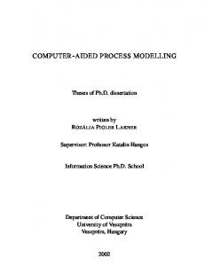
thrusts of ILTP is to reduce the car dependency and increase the share of sustainable travel modes such as walking, cycling and public transport (Queensland Government 2000), as shown in Figure 1.1. However, in order to bring other forms of transport in the level capable of competing with car, it is necessary to substantially improve the transport infrastructure and facilities related to these modes. Before starting the implementation to achieve these objectives, one would certainly like to be sure under what conditions (level of infrastructure, facilities, cost, level of comfort, etc), an individual would like to switch from car to an alternative travelling mode. Therefore, certain potential measures need to be identified that can be put into practice in order to attract a substantial number of car users to adopt public transport to fulfil their travelling needs. The main purpose of this research was to develop mode choice models which can reflect the current travel behaviour of the residents of Redland Shire and forecast the mode shares under different travel scenarios. These travel scenarios could be real or virtual, depending on the data provided by the respondent. For this purpose, a unique computer based travel survey instrument was designed to assess the respondents’ current and future travel behaviours, and further categorised them on the basis of traveller type, i.e. captive (those who perceive to keep using their current mode) or choice users (those who perceive to have a choice). The model specifications developed for the study, for various trip lengths and trip purposes, considered all the commonly used travelling modes in the study area (including access modes for line haul public transport). Several level-of-service attributes of the modes and household parameters, that were surmised to influence the travel behaviour of the targeted population, were tested in order to generate appropriate model specifications for each trip purpose. Various logit models were estimated on the mode choice data, in order to forecast the travel behaviour of the population of the study area, if the hypothetical travel environment, presented in the surveys, can be implemented in practice.
2
90% 80%
78% 69%
70% 60% 50% 40% 30% 20%
15% 6% 8%
10%
10%
6% 8%
0% Car
PT
Walking
Cycling
Current Mode Shares ILTP Target - 2011 Figure 1.1
Current Mode Shares for Journey to Work (2001 Census) and Proposed Mode Shares (ILTP) for Redland Shire
3
1.2. •
HYPOTHESES Disaggregate passenger mode choice models can be developed for various trip lengths and trip purposes, in a multi-modal environment to forecast the travel behaviour using the data obtained through stated preference (SP) surveys.
•
The computer aided survey instrument provides a valid way of understanding residents’ current and future travel behaviour.
•
The modelling process, used in the study, enables the policymakers to test various real and hypothetical travel scenarios.
1.3.
RESEARCH QUESTIONS
The research questions and sub-questions set up for this study are listed as follows, 1. How the values of estimated model parameters vary with the change in the following trip characteristics, ¾ trip purpose i. work; ii. shopping; iii. education; and iv. other. ¾ trip length i. regional (trips near the Brisbane CBD corridor); and ii. local (trips within the Shire). 2. How can a Computer Assisted Personal Interviewing (CAPI) instrument improve the efficiency of the survey design and result in a better response rate from the sample?
4
3. How can the data of the car captive respondents be utilised in analysing the study area’s travel behaviour?
1.4. •
RESEARCH AIMS AND OBJECTIVES To test the feasibility of developing disaggregate passenger mode choice models in a multi-modal environment of the study area, for different trip lengths and trip purposes;
•
To design a computer based stated preference (SP) survey instrument presenting the respondents with real and hypothetical travel scenarios in order to determine the importance they associate with each attribute of the travelling mode used in the model specification;
•
To generate a survey sample, with an apposite size, that can be representative of the whole population of the study area;
•
To determine the sensitivity of various modal parameters, in order to identify their relative influence on the travel behaviour;
•
To forecast the travel behaviour of population of the Shire for unique trip lengths and trip purposes; and
•
To statistically analyse the data obtained from captive users and determine their relative influence on the future travel behaviour.
1.5.
CONTRIBUTION TO NEW KNOWLEDGE
Modelling a Virtual Multimodal Travel Environment Previous stated preference (SP) mode choice studies have generally forecasted the travel behaviour of the targeted population in the presence of a hypothetical motorised alternative for car, such as a high-speed train or a bus on busway (Gunn et al. 1992, Yao et al. 2002). This study focuses on using both motorised (bus on busway) and non-motorised travelling modes (walking on walkway and cycling on cycleway) as alternatives to car. Additionally, a unique choice set of access modes for bus on busway was also generated, containing five hypothetical modes such as
5
secure park and ride facilities and kiss and ride drop-off zones at the busway stations, walkway and cycleway facilities to access the busway stations and a frequent and integrated feeder bus network within the Shire. Therefore, this research modelled a totally new virtual multimodal travel environment for the population of Redland Shire, in order to record their perceived observations under these scenarios and develop the mode choice models. Statistical Analysis of Mode Captive Data Generally, the travel behaviour of members of an affluent society is highly influenced by car (Australian Bureau of Statistics 2002). A big part of the targeted population is generally car captive users, who are not likely to switch from cars to public transport; even if a more efficient transit infrastructure is implemented. In the past, the models have been generally calibrated using the mode choice survey data, while that of the captive users were ignored. This yields a knowledge gap in capturing the complete travel behaviour of a region, since the question of what particular biases can be involved with each model estimation parameter by the captives remain unresolved. Therefore, in this study, various statistical analyses were carried out on the mode captive users’ data by categorising the survey sample, on the basis of different trip characteristics (trip purposes and trip lengths), household characteristics (household size, car ownership level, age-groups, etc) and work trip destinations, in order to determine their relative influence on the travel behaviour forecasts. Additionally, the mode captive users for work trips were further classified according to two types of trip-makers; one of who strictly have to use car as part of their work requirement, and those who currently do not perceive to have choice when presented with mode choice scenarios in the SP survey. It is probable that the latter set of respondents may shift from car to an attractive alternative mode, if the travel environment can be practically implemented. Variation in Travel Behaviour Forecasts for Different Trip Types Despite the development of various passenger mode choice models to forecast the travel behaviour in the past, little has been done to jointly analyse the sensitivity of the travel behaviour of the population with characteristics of the trips undertaken. In order to forecast the modal splits of a study area with a higher degree of accuracy, mode choice modelling needs to be done using these characteristics, by categorising 6
the model specification into different trip lengths and trip purposes. In this study, unique logit models were developed for four trip purposes (work, shopping, education and other trips), and with two trip lengths (trips destined on the Brisbane CBD corridor, known as regional trips, and those undertaken within the Shire, known as local trips). The modelling results for work trips, for instance, showed that the travel behaviour forecasted for regional trip-makers is considerably different from that of local tripmakers. The regional work trip-makers were found not to perceive the non-motorised modes as valid alternatives to car, possibly due to longer trip lengths. The value of time (VoT) determined for local work trip-makers (16.50 A$/hr) was also found to be higher than that of regional work trip-makers (11.70 A$/hr), establishing that mode choice modelling should not only be categorised according to the trip purposes, like in previous studies, but also according to the trip lengths.
1.6. •
SIGNIFICANCE OF THE RESEARCH The research assists in developing a comprehensive understanding of the travel behaviour of the residents of the study area;
•
The research analyses the travel profile of the population in detail, by splitting it into the two traveller types of captive and choice users and statistically examining the influence of various level-of-service attributes and household parameters in the mode choice for different trip purposes; and
•
The research tests the feasibility of developing separate busways, with an integrated network of access modes, and a network of walkways and cycleways.
1.7.
STRUCTURE OF THE THESIS
The methodology for this research was developed using the state-of-the-art travel demand modelling approach, as graphically shown in Figure 1.2. The thesis is also structured following the same order, as shown in the figure.
7
Chapter 1 starts with defining the background knowledge of the research, along with establishing the hypotheses and the research problem. Further, the aims and objectives of the research, and the questions the research aims to answer are also mentioned. The research questions further gave rise to the need for conducting a state-of-the-art literature review on mode choice modelling and stated preference surveys. The main findings from the literature review are respectively shown in Chapters 2 and 3. In Chapter 2, it was established that the logit models are the most commonly used travel demand models, due to their simple formulation and estimation techniques. Therefore, various logit models were developed to estimate the mode choice data and forecast the travel behaviour, for various trip purposes and trip lengths, as shown in Chapters 7 and 8. In Chapter 3, computer assisted personal interviewing (CAPI) was found to be the most commonly used surveying technique, among the transport planners, due to its attractive graphical design and high response rate. Moreover, WinMint 3.2F, a standard CAPI instrument designing software, was selected for designing the survey for this study. Various sample generation methods were also studied in order to find the most appropriate survey sample for the study area, resulting in the selection of the method of stratified random sampling due to its simple theoretical framework and the capability to accurately generate a representative sample for a study area, as compared to other sampling techniques. The southern region of Redland Shire was selected as the study area for this research. Chapter 4 presents various demographics and statistical profiles of the study area in detail, along with demonstrating the key reasons for choosing this region for the research. The design of the stated preference (SP) survey instrument developed for this study is presented in Chapter 5, along with a simple demonstration of how a CAPI mode choice game is presented to the respondents. The findings from the pilot survey, conducted in the study area with a small sample size, are also presented indicating towards the possible editions in the survey instrument design. Chapter 6 further illustrates the implementation strategy adopted for conducting the main surveys in the region and the statistical analyses performed on the survey sample and the data. 8
Research Problem
Research Aims & Objectives
Mode Choice Modelling
Stated Preference Surveys
-
-
Profile Demographics
Model Development Model Specification
Literature Review
Study Area Selection
SP Survey Instrument Design
Pilot Surveys
Main Survey Implementation
Mode Choice Modelling
Captive Analyses
Thesis Writing Figure 1.2
Research Methodology
9
The travel characteristics of the survey sample were compared with the current travel properties of the residents of the study area, taken from the 2001 Census results, shown in Australian Bureau of Statistics (2007b) in order to ensure that the sample is representative of the entire study area. After conducting the SP surveys, the data obtained was categorised according to the traveller type, i.e. the respondents perceiving to have a choice for car, known as choice users, and those who do not, commonly referred to as car captive users. The mode choice data was then, used to estimate various logit models, presented in Chapters 7 and 8, for regional and local trips respectively. The model specifications developed for all the models, i.e. work, shopping, education and other trips, are presented in Chapters 7 and 8 for regional and local trips respectively, along with the estimated coefficients and their sensitivities influencing the travel behaviour forecasts for the study area. Chapter 9 shows various statistical analyses carried out on the survey data by splitting it into the three traveller types of choice, car captive and PT captive users, and categorising them according to several travel characteristics and household parameters. The main findings of the whole research are summarised in Chapter 10, evaluating the results in contrast with the research aims and objectives, as set out in Chapter 1. A direction for future research is also presented, identifying the implementation of the results of this study in a four-step modelling framework. Finally, the references cited through out the thesis are listed.
10
2
Mode Choice Modelling
2.1.
INTRODUCTION Modelling is an important part of most decision-making processes … It is concerned with the methods, be they quantitative or qualitative, which allows us to study the relationships that underlie decision-making. (Hensher and Button 2000)
Transportation is vital for sustaining economic development. Considerable investments have been made in transportation planning and policymaking in order to forecast the future demand of travel. This forecasting needs to incorporate the designing of transportation systems, by making use of the existing infrastructure and the travel behaviour of the residents of the study area. These designing and forecasting techniques for strategic transport planning can be mathematically enumerated and grouped together as transport modelling. Transport modelling plays a key role in the complex system of transport planning and policymaking that can be examined from Figure 2.1.
11
PROBLEM DEFINITION Data Collection System Resources
Objectives
TRANSPORT MODELS Alternatives
Criteria
Consequences Evaluation Selection
Constraints
Figure 2.1
Implementation
Monitoring
Role of Transport Modelling in Policymaking (Modified from Richardson (2003) )
The fundamentals of transport modelling were developed in the United States during the 1950s, and were then imported into the UK in the early 1960s. Thereafter, the following 20 years saw important theoretical developments in the field of transport modelling leading to further work in specific sub-areas. A contemporary dimension was the development of transport mode choice models representing the behaviour of travellers of the study area. Since then, the interest in this field, as well as the growing complexity has led to further development of various travel demand models. However, most of these models trace their origin back to the classical transport demand model, the four-step model (FSM), because of its overarching framework and logical appeal. The basic structure of the model is illustrated in Figure 2.2.
12
Trip Generation
Trip Distribution
Modal Split
Trip Assignment
Evaluation
Figure 2.2
Structure of Four-Step Model
(Modified from McNally (2000) )
This chapter presents a state-of-the-art literature review on passenger mode choice modelling, with particular focus on logit modelling specifications and estimation techniques. The literature review was carried out keeping in mind the development of various mode choice models to forecast the travel behaviour of Redlands, the study area selected for the research, in the travel environment of the Integrated Local Transport Plan (ILTP), as proposed in Redland Shire Council (2002). The models developed contained various modal parameters and household attributes, which were perceived to influence the travel behaviour of the study area, based on previous mode choice modelling studies and the travel scenarios proposed in the ILTP. The literature reviewed in Section 2.2 includes work related to the broader topics of public transport demand modelling, particularly in context of the four-step model with each stage discussed in detail. Sections 2.3 and 2.4 illustrate the theoretical framework and estimation techniques of various modal split models, along with selecting a particular discrete choice model in order to forecast the travel behaviour for this study. Finally, Section 2.5 summarises the main findings from the literature review revealing the research framework, designed to forecast the travel behaviour of the study area.
13
2.2.
FOUR-STEP MODEL
The four-step model has been extensively used in transport demand modelling because of its indispensable rationale as being an overarching design framework. The approach starts by considering the study area as a network of various zones partitioned in order to attain an unbiased data sample from the population. The data is used to estimate a model of the total trips generated and attracted by each zone (trip generation), allocation of these trips to different destinations (trip distribution), modelling the choice of mode (modal split) and allocating the trips by each mode to their corresponding networks (trip assignment). Hence, the model depicted in Figure 2.2 consists of four elementary stages, where each stage addresses an intuitively reasonable query: how many travel movements will be made, where will they go, by what mode will the travel be carried out, and what route will be taken? 2.2.1. Trip Generation The trip generation stage of the classical transport model aims at predicting the total number of trips generated by and attracted to each zone of the study area. Since, it essentially defines the total travel in the study area, it is after trip generation analysis that the transportation planner comes up with the vital figures about the total number of trips generated and attracted by each zone, purposes of these trips, and the travelling modes generally used for these trips. Ortuzar and Willumsen (2001) have demonstrated common trip generation patterns on the basis of following standard trip purposes, •
Work trips;
•
Educational trips;
•
Shopping trips; and
•
Other trips (social, recreational, medical, bureaucratic trips etc.).
14
The most commonly used analytical technique to develop the trip generation patterns of a study area is multiple linear regression. In this technique, the dependent output variable is assumed to have a linear dependence on the independent input variables, which may or may not influence the trip generation, as shown in Equation 2.1. Y = β0 + β1X1 + β2X2 + …. + BkXk + E
(2.1)
where, β0,1,…,k
are coefficients of regression;
X1,2,…k
are independent input variables;
Y
is the dependent output variable; and
E
is the error in estimating the output variable.
The definitions of the input and output variables vary with the type of linear regression approach used in the research. Generally, two types of regression techniques are applied in multi-modal transportation planning namely, •
Zonal-based Multiple Linear Regression; and
•
Household-based Multiple Linear Regression.
The main difference between the two techniques is that the former is used to generate the travel patterns on zonal basis, while the latter does it at an household level. Therefore, for zonal-based regression, Y is generally taken as the number of trips generated for and attracted by each zone in the study area, while various independent variables can be considered and tested for estimation purposes such as, •
employment density of a zone1 (for work trips);
•
school / university enrolment of a zone (for education trips); and
•
shopping areas in a zone (for shopping, work, other trips).
1
The employment density of a zone can be further on the basis of the number of white-collar and blue-collar workers, if desired.
15
Similarly, household-based regression tends to utilise various parameters associated with a household, in order to estimate the regression coefficients, such as, •
household size;
•
number of vehicles in a household;
•
number of adults in a household; and
•
number of workers and students in a household.
Standard literature on statistical techniques and analysis of multiple linear regression can be found in Cohen et al. (2003). 2.2.2. Trip Distribution The trip distribution stage of the four-step tends to provide a standard pattern of trip making by recombining the trip ends with the origins. The trip distribution model is essentially a destination choice model and generates a trip table, for each trip purpose utilised in the model as a function of activity-system attributes and network attributes. This trip table, also commonly known as Origin-Destination Matrix (O-D Matrix), provides a comprehensive illustration of the number of trips generated between different zones of the study area. A number of efforts have been made by transport researchers for developing efficient and adaptive algorithms in order to optimise the O-D Matrix for achieving realistic results. Nielsen (1994) presented two new methods for trip matrix estimation; namely Single Path Matrix Estimation (SPME) and Multiple Path Matrix Estimation (MPME), and demonstrated that the traffic models can be easily and cheaply estimated using them. Three different approaches to O-D Matrix estimation were reviewed and compared, in the context of transport planning, by Abrahamsson (1996) who attempted to use the trip assignment parameters to calibrate the O-D matrix of the study area. Later, Abrahamsson (1998) illustrated an O-D matrix for Stockholm, Sweden that can reproduce the traffic counts, in terms of the number of trips generated and attracted, using the previous distribution approaches improving the accuracy of forecasting of O-D Matrices. Various computationally efficient algorithms for estimating the trip distribution matrices were developed by Safwat and
16
Magnanti (2003) by using a simultaneous approach to develop a four-step model rather than the conventional sequential method. Further, Ber-Gera and Boyce (2003) developed a trip origin based algorithm for transportation forecasting models that combine travel demand and network assignment variables in order to improve the existing O-D flow models. Sherali et al. (2003) developed a non-linear approach to estimate the O-D trip matrices by implicitly determining the path decomposition of a network flow using a sequential linear programming approach. The challenge for researchers in this area, in the immediate future, continues to be the development of a standard optimised algorithm for forecasting accurate and realistic trip distributions. 2.2.3. Modal Split The choice of transport mode is probably one of the most important classic models in transport planning. This is because of the key role played by public transport in policy making. (Ortuzar and Willumsen 2001) The issue of selecting the most appropriate travelling mode has always been a critical issue in travel behavioural modelling, since it tells an individual about the most efficient travelling mode available. Therefore, it is vital to develop and use models that are receptive to those attributes of travel that influence a certain individual’s choice of mode. The quantification of this interaction in terms of mathematical relationships is known as modal split and the travel demand models are referred to as modal split or mode choice models. Hence, the modal split assists a transport planner to assess the impact of each urban element on mode choice and permits testing and evaluation of various transportation schemes. For the model to be representative of the behaviour of the population of the study area, it is essential that survey implementation should be carried out in the study area to record travel data to be used for model calibration, rather than using the data from previous case studies (Richardson 2003). It raises a critical issue of appropriately designing a survey instrument that can record the required travel information of each respondent in the study area, as discussed in Chapter 3. 17
Various discrete mode choice models, generally used for travel behaviour forecasting, are presented in Section 2.3 discussing and comparing their specific features in detail. 2.2.4. Trip Assignment Trip assignment is the last stage of the four-step model, dealing with the allocation of a given set of trip interchanges to a specific transport network. Its main objective is to estimate the traffic volumes and the corresponding travel times or costs on each link of the transportation system by the help of inter-zonal or intra-zonal trip movements (determined by trip generation and distribution) and the travel behaviour of the individuals (determined by modal split). Patriksson (1994) has presented a list of useful purposes of trip assignment in context with transport planning namely, •
assessing the deficiencies in the existing transportation system of the study area;
•
evaluating the effects of limited improvements and extensions to the existing transportation systems;
•
developing construction priorities for the existing transportation system of the study area; and
•
2.3.
testing alternative transportation system proposals.
MODAL SPLIT MODELS
2.3.1. Theoretical Framework A behavioural model is defined as one which represents the decisions that consumers make when confronted with alternative choices. These decisions are made on the basis of the terms upon which the different travel modes are offered, i.e. the travel times, costs, and other level-of-service attributes of the competing alternative travelling modes. The models that tend to represent the travel behaviour of the individuals when provided with a discrete set of travelling alternatives are commonly known as discrete choice models.
18
An individual is visualised as selecting a mode which maximises his or her utility (Ben-Akiva and Lerman 1985). The utility of a travelling mode is defined as an attraction associated to by an individual for a specific trip. Therefore, the individual is visualised to select the mode having the maximum attraction, due to various attributes such as in-vehicle travel time, access time to the transit point, waiting time for the mode to arrive at the access point, interchange time, travelling fares, parking fees etc. This hypothesis is known as utility maximisation and all the travel demand models, presented in this section, are based on this theory. As a matter of computational convenience, the utility is generally represented as a linear function of the attributes of the journey weighted by the coefficients which attempt to represent their relative importance as perceived by the traveller. A possible mathematical representation of a utility function of a mode m is shown in Equation 2.2 as, Umi = θ1xmi1 + θ2xmi2 + …… + θkxmik
(2.2)
where, Umi
is the net utility function for mode m for individual i;
xmi1, …, xmik are k number of attributes of mode m for individual i; and θ1, …, θk
are k number of coefficients (or weights attached to each attribute) which need to be inferred from the survey data.
The choice behaviour can be modelled using the random utility model which treats the utility as a random variable, i.e. comprising of two distinctly separable components: a measurable conditioning component and an error component. Therefore, Umi = Vmi + Emi
(2.3)
where, Vmi
is the systematic component (observed) of utility of mode m for individual i; and
Emi
is the error component (unobserved) of utility of mode m for individual i. 19
For equation 2.3 to be correct, certain homogeneity is needed within the population under study. In principle, it is required that all the individuals share a universal set of alternatives and face the same constraints. Furthermore, in practical modelling work, the difference between the socioeconomic characteristics of similar groups of individuals is usually ignored (Ortuzar and Willumsen 2001). Although this approach makes the whole process simple overall, there is still a possibility of occurrence of severe differences among various groups of people. This can be handled by segmenting the entire set of individuals into separate utility functions for each group of more similar individuals so that individual characteristics could be omitted from the utility function. By ignoring the attributes of the decision maker, the systematic component of the utility can be treated as a function of attributes of available modes only. Therefore, a single utility function can be visualised to exist for all individuals. Similarly, the error component of the utility can also be considered independent of socioeconomic characteristics for the same reason. Assuming that the error component has zero mean and an extreme value distribution (Kilburn and Klerman 1999), the net utility function can be given as: Um = Vm + E m
(2.4)
Thus, if there are M number of total travelling modes available, the probability of an individual selecting mode m, such that m Є M, is based on its associated utility function Um, such that, Um ≥ Ui
(2.5)
where, Um
represents utility of travelling alternative m; and
Ui
represents utility of any travelling alternative in the set of available travelling modes.
Summarising the theory of utility maximisation presented in Equation 2.5, every alternative associates a certain utility with itself determined by its various attributes and an individual is supposed to select the alternative possessing the highest utility. 20
However, it is impractical to assume that the effects of all the variables in an individual’s decision regarding the selection of a travel mode are perfectly understood. The beauty of a random utility model is that it possesses the power to estimate the effects of the observed variables without fully concerning that of the unobserved ones incorporating all of them into the error component of the model, as shown in Equation 2.4. 2.3.2. Logit Models Logit models are the most commonly used modal split models in the area of transportation planning, since they possess the ability to model complex travel behaviours of any population with simple mathematical techniques. The mathematical framework of logit models is based on the theory of utility maximisation and is discussed in detail in Ben-Akiva and Lerman (Ben-Akiva and Lerman 1985). Briefly presenting the framework, the probability of an individual i selecting a mode n, out of M number of total available modes, is given as,
exp(Vin) Pin = ∑ exp(Vim) mεM
(2.6)
where, Vin
is the utility function of mode n for individual i;
Vim
is the utility function of any mode m in the choice set for an individual i;
Pin
is the probability of individual i selecting mode n; and
M
is the total number of available travelling modes in the choice set for individual i.
All logit models are specified on the basis of Equation 2.2 and are applied according to Equation 2.6. The theoretical framework of logit models is based on three main assumptions regarding the error term Em, as shown in Equation 2.4. The assumptions are listed as follows, •
Em is Gumbel distributed;
•
Em is independently distributed; and
•
Em is identically distributed.
21
All these three assumptions serve as the main postulates of the structure of logit models. The first assumption of the random component being Gumbel distributed indicates that all the utilities associated with the travelling modes should be considered as a linear sum of attributes and have the same scale parameter (BenAkiva and Lerman 1985). The last two assumptions are normally grouped together to be referred to as a property of Independence of Irrelevant Alternatives (IIA property), simply meaning that all the travel modes used in modelling the travel behaviour are independent of each other. Logit models are generally classified into two main categories namely binary and multinomial logit models. Binary choice models are capable of modelling with two discrete choices only, i.e. the individual having only two possible alternatives for selection, where as the multinomial logit models imply a larger set of alternatives. 2.3.2.1.
Binary Logit Models
The mathematical framework of a binary logit model is a simplified representation of Equation 2.6 with the total number of available alternatives limited to two, i.e. M = 2. An example of a binary logit model is shown in Figure 2.3 where the choice set contains car and public transport as two competing alternatives.
Choice
Car
Figure 2.3
Public Transport
Example of a Simple Binary Logit Model
22
Simplifying Equation 2.6, the probability of individual i selecting the mode m out of two available travelling modes m and n is given as,
Pim =
exp(Vim ) exp(Vim ) + exp(Vin )
(2.7)
Pim =
1 1 + exp(Vin − Vim)
(2.8)
Pin = 1 – Pim
(2.9)
or,
and,
where, Vim
is the utility function associated to alternative m for individual i;
Vin
is the utility function associated to alternative n for individual i;
Pim
is the probability that alternative m will be selected by individual i; and
Pin
is the probability that alternative n will be selected by individual i.
The main limitation of the binary logit model, shown above, is that it is supposed to be only applied if the travelling alternatives in the choice set are independent of each other. However, when there are groups of more similar or correlated modes, the assumption of having an independent and identical error term across all the modes does not always remain valid. In these cases, a nested logit model can be used that relaxes the constraints of the simple logit models by allowing correlation between the utilities of the alternatives in common groups. The structure of a nested logit model is characterised by grouping all the subsets of correlated alternatives in hierarchies or nests. Each nest, in turn, is represented by a composite alternative which competes with the others available to the individual. An example of a nested logit model, an extension of Figure 2.3, is presented in Figure 2.4 by nesting the two elementary and identical modes of bus and train into the composite mode of public transport.
23
Choice
Public Transport
Car
Bus
Figure 2.4
Train
Example of a Nested Binary Logit Model
The theoretical framework of the nested logit model is based on the same assumptions as the multinomial logit model, except that the correlation of error terms is assumed to exist among various modes. Due to the tree structure of these models, Equation 2.6 is reassessed and is mentioned in Daly (1987), for trees having two levels, as, Pij = Pi . Pj|i
Pj|i =
exp(Vj|i )
∑ exp(Vk|i)
(2.10)
(2.11)
k∈C( i )
Pi =
exp(Vi )
∑ exp(Vt )
(2.12)
t∈R
24
Vj|i = Xj|i
(2.13)
Vi = Xi + hi ln
∑ exp(Vk|i)
(2.14)
k∈C( i )
where, C(i)
is a set of lower-level alternatives that each form part of the higher-level alternative i;
R
is the set of higher-level alternatives;
Xj|i
is the measured attractiveness of alternative j conditional on i;
Xi
is the measured attractiveness of alternative i; and
hi
is the scale parameter.
2.3.2.2.
Multinomial Logit Models
Similar to binary logit models, the multinomial logit models are also categorised into simple and nested multinomial logit models, based on the characteristics of the available travelling alternatives in the choice set. The examples of simple and nested multinomial logit models are presented in Figures 2.5 and 2.6 respectively.
Choice
Car
Figure 2.5
Cycle
Walk
Bus
Example of a Simple Multinomial Logit Model
25
Choice
Car
Car as Driver
Cycle
Walk
Car as Passenger
Figure 2.6
Bus
Walk
Car
Example of a Nested Multinomial Logit Model
The multinomial logit models use the same mathematical framework as shown in Equations 2.2 to 2.14 and are generally estimated using maximum likelihood method, discussed in Section 2.4.1. 2.3.3. Probit Models Certain situations can occur where the utilities of some alternatives are correlated in a complex way or possess different variances. In these cases, the multinomial logit models can make erroneous forecasts regarding the probabilities of mode shares when the attributes associated to one or more travelling alternatives are varied. The probit model has been proposed as one of the possible methods to overcome this problem. The model follows normal distribution for error terms and does not work under the strict assumptions as that of logit models. Similar to logit models, the probit model is also based on random utility theory, representing the utility function as the sum of the systematic component and an error component. The standard equation for the utility of an alternative i has the form (Horowitz 1991) as shown in Equation 2.15, 26
Ui = V(xi,s) + εi
(2.15)
where, Ui
is the utility of alternative i;
V
is the systematic (observed) component of the utility function;
ε
is the error (unobserved) component of the utility function;
xi
is the vector of observed attributes of alternative i; and
s
is the vector of observed characteristics of the individuals of the study area.
Due to the complex estimation algorithms of probit models, the transport planners generally prefer using logit models as they possess simple mathematical framework and can accurately model the travel behaviour of a study area. Ghareib (1996) compared logit and probit models by using them to estimate the travel behaviour for different cities of Saudi Arabia and concluded that the logit models are superior to their probit counterparts in terms of their goodness-of-fit measures and tractable calibration. Dow and Endersby (2004) later supported his findings by concluding that the logit models should always be preferred over probit models and the latter should only be utilised if the travel behaviour of the targeted population to be determined is observed to be complexly correlated. 2.3.4. General Extreme Value Models In an important simplification of multinomial logit models, generalised extreme value (GEV) models were developed based on the stochastic utility maximisation. Although there exist a limitless number of possible models within this class, only a few have been truly explored. This model is based on a function G(y1, y2, …, yJn), for y1, y2, …, yJn ≥ 0, that has to satisfy certain conditions discussed in detail in Ben-Akiva and Lerman (1985). The basic equation of the model is given as,
Pn(i) =
exp(Vin ).Gi(exp(V1n ), exp(V 2 n ),..., exp(VJnn )) μG (exp(V1n ), exp(V 2 n ),..., exp(VJnn ))
(2.16)
27
where, V
is the systematic (observed) component of the utility function;
μ
is the degree of homogeneity; and
Pn(i)
is the probability of individual n selecting alternative i.
In addition to the three modal split models discussed above, there also exist a few discrete choice models which can be referred as the generalisations of logit models, namely Random Coefficient Logit, Tobit and Ordered Logistic models. Due to the occurrence of high limitations in the specifications and estimation complexities of these models, they are rarely put into practice by transport planners. A detailed mathematical framework of these models is presented in Ben-Akiva and Lerman (1985) and Amemiya (1994). 2.3.5. Comparison of Modal Split Models The first step in modal split modelling is to generate a travel profile of the study area and determine a representative choice set, based on the travel characteristics of the targeted population. The size of the choice set determined assists in the selection of an appropriate mode choice model in order to forecast the travel behaviour of the study region. If the choice set consists of two travelling modes, or two sets of travelling modes, a binary modal split model can be applied. Contrarily, multinomial modal split models can be selected for bigger choice sets. This classification of the discrete mode choice models on the basis of the choice set is illustrated in Figure 2.7.
28
Mode Choice Models
Binary Choice Models
Binary Logit Model
Simple Binary Logit Model
Multinomial Choice Models
Binary Probit Model
Nested Binary Logit Model
Figure 2.7
Multinomial Logit Model
Simple Multinomial Logit Model
Multinomial Probit Model
General Extreme Value Model
Nested Multinomial Logit Model
Classifications of Mode Choice Models
Various disparities among the three most common mode choice models, namely the logit, probit and general extreme value models, are tabulated in Table 2.1, identifying the main distinguishing factors among the specifications and applications of these models.
29
Table 2.1
Comparison of Common Mode Choice Models
Logit
Probit
General
Models
Models
Extreme Value Models
Basic
Extreme Value
Normal
Multivariate
Hypothesis
Distribution
Distribution
Extreme Value Distribution
Error terms should
Error terms need not
Error terms need
Major
necessarily be
necessarily be
not necessarily be
Constraints
identically and
identically and
identically and
independently
independently
independently
distributed
distributed
distributed
Simple
Complex
Complex
Simple
Complex
Complex
Introduction
Model formulation
Model formulation
Model
of
and calibration
and calibration
formulation and
Access
becomes complex to a
becomes highly
calibration
Modes
small degree
complex
becomes highly
Model Formulation Model Estimation
complex
Application
High
Limited
Limited
Accuracy
High
Low
Low
Table 2.1 shows the general reasons of why the logit models are most commonly used among the transportation planners for estimating and forecasting the travel behaviour of a study area. The specifications developed for logit models associate certain limitations due to the IIA property, discussed in Section 2.3.2; however, the main reasons for choosing them are their simple model formulation and estimation techniques. Other mode choice models such as probit and general extreme value models have relaxed the IIA restriction at the cost of possessing highly complex mathematical structure and computational estimation. Therefore, the logit models continue to remain dominant in the transport modelling arena. 30
2.4.
MODEL ESTIMATION TECHNIQUES
Generally, two model estimation techniques are used for estimating the discrete mode choice models, in order to infer the values of the unknown coefficients θ1, θ2, … , θk shown in Equation 2.2, namely the maximum likelihood and least squares method. Brief model formulations of these models are presented in Sections 2.4.1 and 2.4.2 respectively. A detailed literature of the theoretical framework, applications and limitations of these models is presented in Greene (2003). 2.4.1. Maximum Likelihood Method The method of maximum likelihood is the most common procedure used for determining the estimators in simple and nested logit models. Stated simply as, The maximum likelihood estimators are the values of the parameters for which the observed sample is most likely to have occurred. (Ben-Akiva and Lerman 1985) The method requires a sample of individual mode choice decision-makers along with the data regarding the travelling mode chosen and the attributes of that particular mode. The basic formulation of the method, that involves the maximisation of the likelihood function, is shown in Equation 2.17 as, M
L=
∏ P(tm, m)
(2.17)
m =1
where, L
is the likelihood the model assigns to the vector of available alternatives;
M
is the total number of available alternatives;
m
is any alternative present in the set of available alternatives;
tm
is the mode observed to be chosen in alternative m; and
P(tm,m) is the probability for choosing alternative m.
31
The most widely used approach is to maximise the logarithm of L rather than L itself. It does not change the values of the parameter estimates since the logarithmic function is strictly monotonically increasing. Thus, the likelihood function is transformed to a log-likelihood function and is given as, M
L1 =
∑
log [P(tm,m)]
(2.18)
m =1
Given the mode choice data, most existing estimation computer programs estimate the coefficients that best explain the observed choices in the sense of making them most likely to have occurred. Standard commercial packages such as ALOGIT (Hague Consulting Group 1992) are generally implied for estimating logit models, mostly due to their capability of handling complex nested logit structures, both linear and non-linear. 2.4.2. Least Squares Method The method of least squares is generally stated as, The least square estimators are the values that minimise the sum of squared differences between the observed and expected values of the observations. (Ben-Akiva and Lerman 1985) The coefficients of regression are estimated by the basic objective function F which is given by (see Equation 2.1), F = min ∑ E2 = min ∑ (β0 + β1X1 + β2X2 + …. + BkXk – Y)2
(2.19)
The desired coefficients are estimated by taking (k+1) derivatives of equation 2.19 and solving for (k+1) unknowns. This method is usually called the Ordinary LeastSquares (OLS). Generally, the least-squares estimators are unbiased under general assumptions. However, it should be noted that the least-square method works consistently and efficiently for linear models only, and can surmise erroneous
32
coefficients’ values in case of complex model specifications. Therefore, due to its higher applications, the maximum likelihood method is generally preferred over the least square method by the transport statisticians and planners.
2.5.
SUMMARY
This chapter presented the main findings of the state-of-the-art literature review conducted on passenger mode choice modelling in a travel behavioural framework. The main aim of appraising the literature was to determine a modal split model that can be implied to forecast the travel behaviour of the population of Redland Shire, study area selected for the research, under the ILTP travel environment. Firstly, the four-step model was reviewed since it is regarded as the basic overarching framework for travel demand modelling. Each step of the model was briefly discussed, with major focus on mode choice where the theoretical framework and main properties of various discrete choice models were examined. It was concluded that logit models associate the most practical modelling framework, out of all modal split models, although they are based on the IIA property which assumes that all the travelling modes used in the choice set are independent of each other. This condition is, however, relaxed with the use of a tree structure that combines the correlated modes into one nest. Logit models are generally classified into two main categories, namely the binary and multinomial logit models, depending on the size of the choice set generated for the study area. For choice set presenting two travelling alternatives to the targeted population, a binary logit model was preferred. Contrarily, multinomial logit models were implied for bigger choice sets. Maximum likelihood method was found to be the most commonly used estimation technique for logit models, due its ability to handle complex structures. Computer estimation packages such as ALOGIT are generally used for model calibration purposes, mainly due to their capability to perform numerous mathematical iterations using various statistical techniques.
33
3
Stated Preference Travel Surveys
3.1.
INTRODUCTION Economists typically display a healthy scepticism about relying on what consumers say they will do compared with observing what they actually do; however, there are many situations in which one has little alternative but to take consumers at their words. (Louviere et al. 2000)
The standard framework of travel demand modelling requires data which can precisely reflect the travel characteristics of the targeted population. This data can be gathered by conducting surveys in the study area, asking the respondents regarding the attributes associated to their current or future travelling modes. This data may also involve elicitation of various travel preferences and choices, identifying the respondents in the survey sample having choice over a certain mode. This elicitation needs to be realistic and practical in order to forecast the travel behaviour with a higher degree of accuracy. Therefore, the surveys conducted should not only involve questions regarding essential current travelling attributes but also be capable of observing the behaviour of the respondents when faced with hypothetical attributes and conditions (Stopher and Jones 2003). These surveys are generally referred as stated preference (SP) travel surveys and are generally used in forecasting the travel behaviour of a study area in a hypothetical travel environment. Contrarily, the surveys involving questions regarding the current travelling attributes in a real environment are classified as revealed preference (RP) surveys and thus, can be used to estimate the current travel behaviour of a study area. During the last few years, stated preference methods have become established as one of the key tools of demand analysis as they are frequently adopted by transportation planners for the analysis of the impact of transport policies on travel demand (Fujii
34
and Garling 2003). Some of the main reasons behind this popularity of SP surveys are summarised as follows, •
they can predict travel behaviour of a study area under various hypothetical travel scenarios proposed in the transport policies for that area;
•
they can ensure that the current transport planning reflects all the essential attributes of the travelling modes used in the study area; and
•
they can detect the relative importance of qualitative or latent variables such as comfort, convenience, safety etc, which may be inaccurately estimated by RP data (Ortuzar 1996b).
As stated in Chapter 1, the main aim of this research was to develop mode choice models in order to forecast the travel behaviour of the residents of Redland Shire under hypothetical ILTP scenarios for various trip purposes. Therefore, stated preference (SP) surveys were conducted in the study area in order to observe the perception that the respondents associate to various travelling alternatives to the car. Further, the SP data, obtained from the respondents with mode choice, was entailed in calibrating various logit models for different trip lengths and purposes. The theoretical framework and estimation techniques of logit modelling were discussed in Chapter 2 in detail. This chapter presents the findings of the state-of-the-art literature review conducted on stated preference survey instrument designing, use of pilot survey in finalising the instrument, and sampling techniques to generate a representative set of respondents for the study area. The chapter starts by presenting various physical forms of the survey instrument designs, generally used by the transportation planners. Various instrument forms such as computer-based interviewing, mail-back questionnaires and face-to-face surveying are discussed. After comparing the properties of the physical forms of each survey instrument, Computer Assisted Personal Interviewing (CAPI) were selected for conducting SP surveys in the study area due to their specific design and high response rates. Various advantages of conducting a pilot survey on a small sample size within the study area, before the actual survey implementation, are also discussed. The main benefit of the pilot survey was found to be the editing and finalising of the survey instrument, for the actual survey, based on the reactions of 35
the respondents on the graphical interface of the instrument design. Several techniques for generating the survey sample are also presented and compared, resulting in the selection of the method of stratified random sampling due to its simple theoretical framework and the capability to accurately generate a representative sample for a study area. Finally, a brief discussion on sampling errors and biases is presented, discussing the possible influences of the two on the travel behaviour forecasts for a study area.
3.2.
PHYSICAL FORMS OF SURVEY INSTRUMENTS
The development of a stated preference survey instrument has always been a challenging task for the designers since the travel data needed to be collected by the instrument is entirely dependent on the study area and the behaviour of the residents. It is also essential that the survey instrument should be appropriately designed as to record only the travel data that is vital for model estimation rather than overburdening the respondent with excessive questioning (Sanchez 1992). Further, the selection of appropriate, simple and clear wording for the questions also result in a high response rate for the survey. However, the most vital aspect of the survey instrument is the physical nature of the form on which the data is to be recorded. The survey instruments can be designed by various physical forms depending on the nature of the travel data being collected. Currently, the two common forms in practise are computer assisted and paper-and-pencil survey designing. Other forms such as mail-back and telephone surveys have become dormant since the current ones effectively reduce the survey non-response rates (Murakami et al. 2003) and reflect more genuine travel behaviour (Wermuth et al. 2003). However, the paperand-pencil interviewing is also gradually becoming extinct because of the flexibilities and easiness computer assisted interviewing provides to the interviewers and the respondents.
36
3.2.1. Computer Assisted Personal Interviewing (CAPI) The movement to computer based survey methods is not an option. It seems as inexorable as the transition to computers in most other organised human activities in modern society. (Couper and Nichols 1998) Computer Assisted Personal Interviewing (CAPI) is a computer assisted data collection method used for surveying and collecting data in person. It is usually conducted at the home, workplace or business of the respondent using a portable personal computer, such as a notebook. CAPI can also include Computer Assisted Self-Interview (CASI) session where the interviewer hands over the computer to the respondent for a short period, but remains available for any instructions or assistance for the respondent. After finishing the interview, the data is generally sent to a central computer, where all the survey databases are managed. A block diagram of CAPI survey data recording process is shown in Figure 3.1.
Survey Sample
Survey Instrument (CAPI)
Pilot Survey
CAPI Management System
Previous Travel Behaviour Information
Remote Devices
Results
Survey Implementation Survey Database
Figure 3.1
CAPI Data Collection Process
37
The role of the interviewer is a significant factor in conducting successful CAPI interviews. Wojcik and Hunt (1998) suggested various training techniques for the CAPI interviewers; some of them being maintaining the focus on the administration of the survey instrument, designing the instruments on latest available technologies and developing objective measures for assessing the success of the interviewers in achieving the survey objectives. Sperry et al. (1998) further added to factors of the successful completion and higher response rates of CAPI by stressing the importance of sound communication skills and harmony between the interviewers and the respondents. Additionally, the use of computers in data collection can considerably reduce the amount of work and provide automatic data coding techniques that improve the data quality and thus, estimate the model with a higher level of accuracy. Various standard CAPI instrument designing packages, such as WinMint (HCG 2000), are commonly used by the survey designers, mainly due to their capability of generating random hypothetical SP games based on current travel characteristics of the respondents. 3.2.2. Paper-and-Pencil Interviewing (PAPI) Paper-and-Pencil Interviewing (PAPI) is an orthodox manual method of data collection implemented with the help of the interviewers involved in face-to-face interviews with the respondents. PAPI can also have a mail-back self-interviewing part which is generally filled by the respondents themselves. Contrarily to CAPI, this method involves manual data coding and recording by the designers and interviewers respectively. Therefore, the probability of having errors and biases in the survey instrument design is higher than that of CAPI (Kalfs 1995, Wermuth et al. 2003). Further, examination and comparison of various aspects of PAPI and computer-based surveying using telephones by Bonnel and Nir (1998) suggested that the former is a very expensive method in terms of survey instrument designing, data coding and data recording. Due to these and many other reasons, PAPI are becoming extinct, particularly for surveying in the developed countries. 3.2.3. Other Forms of Survey Instruments Apart from computer assisted and paper-and-pencil interviewing, there also exist various other survey methods for data collection. However, these methods have 38
already become non-existent due to the fact that the current two methods provide higher flexibility for the instrument designers in terms of coding and designing and to the interviewers and respondents in terms of data recording. Some of these methods are briefly described in this section. 3.2.3.1.
Postal Survey
A postal survey, by definition, is another method of self-administered interviewing. Generally, it involves mailing a questionnaire to the respondent’s home by post so that they can mail it back to the survey administration after completing the surveys. As a result, the presence of an interviewer is not required in specific. Although the absence of the interviewer causes the survey to be less expensive, in terms of cost and time, as compared to the current survey methods, it does raise the issue of having no interviewer helping the respondent in answering the questions (Jenkinson and Richards 2004). An excellent detailed comparison of different aspects of postal, face-to-face and telephone interviewing such as survey implementation cost, data sampling, quality control and flexibility along with examples can be found in Bonnel (2001). 3.2.3.2.
Internet Survey
An internet survey is comparatively a contemporary self-interviewing method for data collection in which the respondent is generally supposed to fill the questionnaire over the internet. The identity of the respondent filling the questionnaire is generally unknown and thus, the validity of the data provided by the respondent is usually difficult to determine (Lazar and Preece 1999). Timmermans et al. (2003) and Adler et al. (2002) presented results from an internet based travel survey concluding that although this method offers potential in administering relatively complex tasks such as stated preference experiments, it can be highly unreliable. Therefore, the model estimated from the internet survey cannot be totally judged to generate accurate results. Secondly, the sampling frame for internet surveys is often not available as it cannot be known that the respondents may behave totally differently to the population of interest.
39
3.2.4. Advantages of Computer-based Survey Instrument Sarasua and Meyer (1996) identified the following major advantages that computer assisted interviewing has over other surveying methods, •
interesting and flexible presentation format;
•
consistent format across the interviewers and the respondents;
•
automatic question branching and prompting;
•
automatic data coding and storage; and
•
ability to incorporate checks to avoid inconsistent or wrongly entered answers.
Based on the advantages of implementing CAPI listed above, it is concluded that computer-based surveying is superior to other forms of survey instruments.
3.3.
PILOT SURVEY
A pilot survey is a complete run through of the actual survey, done over a small set of population in order to determine the level of credibility of the instrument, data coding and data recording. Further, analysis of the results is also done along with the calibration of the model so that the data validity could also be properly known. The actual aim of conducting the whole exercise is to identify the potential flaws in the survey instrument design and data recording, observe the response of the respondents and determine the discrete discrepancies in the survey administration before the interviewers begin conducting the actual survey. Although, pilot testing forms one of the most important components of the survey procedure, it is also one of the most neglected because of the lack of time and money on the side of the survey administration. However, Ampt (1993) fully supported the use of pilot surveys by stating that the pilot testing should be done even on those survey techniques and questionnaires which have been used successfully in similar circumstances on anyone other than the target population. Pratt (2003) added that this testing should not be confined to the designer’s work associates but should
40
substantially include people from the same population that are to be surveyed in the main survey. Richardson et al. (1995) described various uses of conducting a pilot survey in detail. Some of them are listed here as follows, •
determine the adequacy of the sampling frame;
•
observe the variability of the parameters within the survey population;
•
examine the causes of the non-response rates;
•
scrutinize the method used for data collection;
•
check the question wording and layout of the questionnaire;
•
study the procedures of data entry, editing and analysis; and
•
swot the cost of the survey.
The size of the pilot survey is a trade-off between cost and efficiency. It cannot be as extensive as the main survey but nevertheless it should be large enough to yield significant results. Richardson et al. (1995) further pointed out a rule of thumb for the survey cost that the survey administration should allocate at most ten percent of the actual survey budget for the pilot survey.
3.4.
SAMPLE GENERATION METHODS
Sample generation is regarded as a vital step in travel demand modelling since the modal split models are generally estimated using the data collected by surveying a sample of respondents from the targeted population. Therefore, it is essential that the sample generated for the research is representative of the characteristics of the population of the study area. Inappropriate sample generation can lead to erroneous modelling results involving biased estimated coefficients and non-representative travel behaviour forecasts.
41
This section discusses and compares various commonly used sample generation techniques, with focus on selecting a suitable method to generate an apposite sample for this study in particular. 3.4.1. Simple Random Sampling Simple random sampling is the simplest approach out of all sample generation techniques and is the basis of all other random sampling methods. In this method, a totally random sample is chosen from the target population, using a sampling frame with the units numbered. Since the sampling is totally random, every member of the target population set has an equal probability of being selected. Therefore, if the set of target population contains N number of members, and the sample is supposed to have n members, provided that n ε N, the probability to generate the sample in n number of draws, using simple random sampling, is presented in Equation 3.1 as,
NPn
=
n! (N − n)! N!
(3.1)
where, NPn
is the probability to select n number of members from a set of N members, such that n ε N.
This method is also known as random sampling without replacement. Further mathematical details of the method are given in Govindarajulu (1999). Although this method is simple, it becomes highly impractical for larger sample sizes. Ampt and Ortuzar (2004) proved that the method often produces highly variable results from repeated applications for high sample sizes. Therefore, the method is only applicable for generating small sample sizes and is limited to simple sampling approaches. 3.4.2. Stratified Random Sampling In stratified random sampling, the targeted population is split into distinct subpopulations, known as strata. These strata are classified on the basis of various factors of relevant interest to the survey and are obtained by simple random sampling 42
within each stratum. For example, for a mode choice survey, the strata can be categorized on the basis of the users of various travelling modes, i.e. the individuals using private cars and public transport (Tsamboulas et al. 1992, Steg 2003). Similarly, the classification can also be done on the basis of various socioeconomic conditions of the households such as structure, age groups and income-levels. Chang and Wen (1994) explain that if the entire population contains N units, then stratified random sampling can be done by dividing it into L number of nonoverlapping strata such that, N1 + N2 + ….. + NL = N
(3.2)
where, N1,2, … , L
are the number of units in each strata L.
Whilst stratified sampling is useful, in general, to ensure that the correct proportions of each stratum are obtained in the sample, it becomes highly significant in identifying relatively small sub-groups within the population. Therefore, it enormously increases the precision of the estimates of attributes of the targeted population of a study area. However, considerable prior information regarding the attributes of the population should be known before generating the sample. 3.4.3. Multi-stage Sampling Multi-stage sampling is a random sampling technique for study areas with large populations. It is based on the process of selecting a sample in two or more successive contingent stages. It proceeds by defining aggregates of the units that are subjects of the survey, where a list of the aggregates is easily available or can be readily created. Richardson et al. (1995) explained the process of multi-stage sampling within Australian context by splitting it into five distinct stages as shown in Figure 3.2.
43
Country (Australia)
Total Population
States
1st – Stage Sample
Local Government Areas
2nd – Stage Sample
3rd – Stage Sample
Census Collectors’ Districts Households
4th – Stage Sample
Individuals
5th – Stage Sample
FINAL SAMPLE
Figure 3.2
Example of Multi-stage Sampling Process
The major disadvantage of multi-stage sampling is its low level of accuracy of the parameter estimates for a given sample size as compared to that estimated using a simple random sample for the same study area. However, the reduction in accuracy is often traded off against the reduction in costs and efficiency in administration of the sampling process that the multi-stage sampling associate. Hossain et al. (2003) proved this argument by presenting various population models based on different sampling techniques, out of which the most efficient method, in terms of application and economy, was found to be multi-stage sampling. 3.4.4. Cluster Sampling Cluster sampling is a slight variation of multi-stage sampling where the targeted population is first divided into clusters of sampling units, and then sampled
44
randomly. The units within the cluster are either selected in total or else sampled at a very high rate. Detailed literature on the theoretical framework of the method, along with some useful examples, is presented in Stehman (1997). Similar to multi-stage sampling, cluster sampling can also be highly economical and administratively efficient as compared to simple random sampling, especially for study areas with large populations. Additionally, if the study areas are well-defined, a transport modeller can easily manage to have a high degree of quality control on the conduct of the interviews. However, the main disadvantage, like multi-stage sampling, continues to be the less accuracy in estimating the coefficients for any given sample size as compared to that estimated using simple random sampling. 3.4.5. Systematic Sampling Systematic sampling is perhaps the most widely known non-random sampling technique among the transport modellers. The method involves selecting each kth member of the targeted population. The first member is chosen randomly and then, after every kth interval, another member is selected to be part of the sample. For example, if the targeted population contains N members and the desired sample size is n, then after selecting the first member randomly, the other members are selected every N/nth interval. However, this constraint does not need to be strictly enforced and can be modified by the modeller according to the level of model complexity. In study areas where the size of the targeted population is very large or almost infinite, Stopher (2000) suggested that every twentieth member of the set should be selected as part of the sample. Although systematic sampling is the easiest and simplest sampling method known, it possesses various limitations. First, and most importantly, the sample set generated using systematic sampling generally contains various biases because the targeted population sometimes exhibit a periodicity with respect to the parameter being measured. This causes the resulting sampling set to be significantly biased towards that certain parameter. The second limitation is the scenario in which the resulting sample set may not effectively represent the users of a certain travelling mode. This situation generally occurs in enormously populous study areas where there is
45
assorted practise of travelling modes and the transport modellers unconsciously ignore these users, causing bias in the sample set. 3.4.6. Comparison of Sample Generation Methods The sections above presented various sample generation techniques that are commonly implied by the transport modellers in order to generate an apposite sample for the study area. The benefits and limitations of each sampling method are presented in Table 3.1 in order to select the most appropriate sampling technique for this study.
Table 3.1
Sampling
Comparison of Sample Generation Methods
Benefits
Limitations
Methods Highly simple and does
Infeasible for study areas
Simple
not involve complex
with large populations.
Random
computer algorithms.
Inconsistent most of the
Sampling
times by giving highly variable results.
Stratified Random Sampling
Useful when data of
Considerable prior
known precision are
information regarding the
wanted for certain
attributes of the
subdivisions.
population is needed
Significant administrative
before the actual
convenience, particularly
sampling can take place.
for transport surveys. Precise estimates of the characteristics of the targeted population.
46
Multi-stage Sampling
Feasible for study areas
Level of accuracy of
having large populations.
parameter estimates for a
At each stage of the
given sample size tends
process, different sampling to be less than if a simple methods can be applied
random sample had been
giving more flexibility to
collected.
the transport modeller. Highly economical and
Less accuracy in
administratively efficient
estimating the
as compared to simple
coefficients for any given
random sampling,
sample size as compared
especially for study areas
to simple random
with large populations.
sampling.
Cluster Sampling
If the study areas are welldefined, a transport modeller can easily manage to have a high degree of quality control on the conduct of the interviews. Simplest of all other
The set of target
methods and is often easier population can exhibit a
Systematic Sampling
to execute.
periodicity with respect
Generally more precise
to the parameter being
than simple and stratified
measured causing bias in
random sampling, since it
the results.
is spread more evenly over
For mode choice study,
the population.
unique travelling mode users may get ignored.
47
Previous SP mode choice studies have suggested that a random sample should be generated in order to minimise the bias that may be attached to a certain mode by the targeted population (Louviere and Street 2000, Parajuli and Wirasinghe 2001). Therefore, the method of systematic sampling was ruled out as it directs at generating a non-random sample from the population of the study area. The major issue with using the methods of multi-stage and cluster sampling was that their main applications are generally limited to study areas with huge populations only. The study area selected for this research, the southern suburbs of Redland Shire, contain a total population of around 55,760 only, according to the 2004 estimate presented in Australian Bureau of Statistics (2007d). Therefore, given the small population of the study area, implying the methods of multi-stage and cluster sampling were not considered for this research. Comparing the remaining two methods of simple and stratified random sampling, it was concluded that the latter generates representative samples with higher level of accuracy. Thus, the sampling technique selected in order to generate an appropriate sample for this study was stratified random sampling with its stratum being the population of each suburb in the study area, as presented in Chapter 4.
3.5.
SAMPLING ERRORS AND BIASES
From the stages of data collection to that of final model estimation, the data are generally subject to various sorts of errors and biases. A sampling error arises simply because of the fact that a modeller deals with a sample rather than with the whole population of a study area. Thus, the sampling error cannot be totally eliminated even if the sample is very carefully selected and the instrument well designed. Richardson et al. (1995) defined sampling error as primarily a function of the sample size and the inherent variability of the parameter under consideration. However, the sampling error generally does not affect the estimated parameter values and merely influence the variability around these averages (Brownstone et al. 2002). 48
Sampling bias is a total different concept from sampling error and arises mainly because of the mistakes made by the modeller in choosing an appropriate sampling method. Having bias in the sample survey results is a more severe problem than sampling error itself since it directly affects the estimated values. The results can get highly unrealistic due to the induction of sampling bias and therefore, forecasting travel behaviour becomes impractical. However, sampling bias can be virtually eliminated by careful attention to the various aspects of sample survey design and by adopting the most appropriate sampling method. In an attempt to improve the accuracy of sample surveys, a modeller needs to be aware of the likely sources of sampling bias and the possible measures to be taken in order to eradicate them. The most significant of these common sources and possible measures are mentioned in detail by Richardson et al. (1995). Some of the significant safeguards against the introduction of sampling bias in travel surveys are listed as follows, •
using a random sampling selection process and fully adopting the sample generated by it;
•
designing the survey instrument in such a manner that there is no need for doing further sampling;
•
performing random call-backs on some respondents in order to check the validity of the travel data obtained by surveying them;
•
performing cross-checks with other secondary sources of data to check on the validity of the responses;
•
increasing the response rates; and
•
having significant information regarding the travel characteristics of the entire sample.
Sampling bias generally varies with the type of survey method used by the modeller and the parameters which the survey seeks to estimate. Therefore, conducting a pilot survey with a small but significant sample in order to determine sampling bias is highly recommended, before the actual survey implementation.
49
3.6.
SUMMARY
This chapter presented the findings of the state-of-the-art literature review conducted on stated preference (SP) survey instrument designing and sample generation techniques. The main aim of reviewing the literature was to determine the most suitable form of the survey design and an appropriate method to generate a representative sample for the study area chosen for this research. Various physical forms of the survey instruments were considered, including the two most common designs of computer assisted personal interviewing (CAPI) and paperand-pencil interviewing (PAPI). CAPI was found to be most famous SP surveying technique among the survey designers due to its graphically attractive presentation format and higher response rates as compared to other surveying methods. WinMint, a software programming tool, was found to be one of the most commonly used CAPI designing packages being used by the survey designers. Moreover, the uses of conducting pilot surveys in the study area were elaborated with the main benefit being the editing and finalising the design of the survey instrument for the actual survey implementation. Similarly, five sample generation techniques were presented in Section 3.4 comparing the benefits and limitations of each method in Table 3.1. For this research, the method of stratified random sampling was deemed as the most suitable sampling technique considering the small population size of the study area. Finally, a brief discussion on sampling errors and biases associated to the various steps of data collection and model estimation was presented. It was found that the sampling errors cannot be totally eliminated from the modelling results, however, they generally have an insignificant influence on the values of the estimated coefficients and the variability around them. Contrarily, sampling bias was found to be a bigger problem than the sampling error since it can substantially affect the travel behaviour forecasts for a study area. However, sampling bias can be virtually eliminated by careful attention to the various aspects of sample survey design and by adopting the most appropriate sampling method.
50
4
Selection and Characteristics of the Study Area
4.1.
INTRODUCTION
For transportation research purposes, a study area is generally regarded as a geographical region in which transport planning needs to be done, for reasons such as estimating and forecasting the travel behaviour of the population. It is essential for a transport modeller to have accurate information and statistics on the boundaries, land features, population growth, and transport infrastructure of the study area. It helps in determining the travelling modes commonly used by the residents, along with their significant attributes. A comprehensive description of defining the study area boundaries for travel surveying purposes is given in Ortuzar and Willumsen (2001). The southern region of Redland Shire (in South-East Queensland) was selected as the study area for this research. This chapter presents various demographics and statistical profiles of the study area in detail. The main reasons for choosing this study area are also discussed. Sections 4.2.1 and 4.2.2 present a thorough description of the study area, with boundaries, transport infrastructure and population statistics. The current travel behaviour of the study area is discussed in detail in section 4.3 with the help of various graphical illustrations on the population and travel profile of the residents of each suburb included in the study area. A brief discussion is provided on how these socio-demographic characteristics and trends are influencing (or may influence) the travel behavioural framework of the population. In the end, Section 4.4 concludes the findings of the chapter by focussing on the main factors that impinge (or are supposed to impinge) on the mode choice decision-making of the travellers for various trip purposes. However, a complete travel profile can only be presented with the help of mode choice modelling results that can forecast the travel behaviour in the ILTP environment as discussed in Chapters 7, 8 and 9.
51
4.2.
STUDY AREA PROFILE
This section shows the map and profile of the study area along with a brief background on the travel behaviour characteristics of the residents. 4.2.1. Selection of the Study Area The study area targeted for the research covers the five southern suburbs of Redland Shire namely, •
Victoria Point;
•
Thornlands;
•
Redland Bay;
•
Mount Cotton; and
•
Sheldon.
This study area was defined and finalised under the supervision of Redland Shire Council. Figure 4.1 shows the map of the suburbs of the Shire that were selected as part of the study area for the research. These suburbs account for around 31 % area of the whole of Shire. The southern part of the suburb of Capalaba, outside the study area, was selected as the control area2 for surveying purposes. Therefore, in addition to the residents of the above five suburbs, the survey sample also contained a significant number of the residents of Capalaba.
2
Control area is defined as a region surveyed for model validation purposes or for conducting additional surveys.
52
Figure 4.1
Map of Redland Shire
53
There were two main reasons for specifically selecting the southern suburbs of the Shire. First pragmatically, the northern suburbs were covered under the TravelSmart study (Queensland Government 2004) and therefore, the Council was not interested in re-conducting a travel survey in these suburbs. Secondly, the study area selected does not have a proposed railway corridor; therefore, the model specification requirements became different as the SP set of hypothetical travelling modes could not contain train as a valid alternative to car. The model specification developed for this research, as discussed in section 4.4, had to be limited to four all-the-way modes (car, bus, walking, cycling), along with five modes to access the public transport (walking, cycling, feeder bus, park & ride, and kiss & ride). However, the number of travelling modes varies among different model specifications for different trip lengths as discussed in chapters 7 and 8. 4.2.2
Study Area Characteristics
Redland Shire is a Local Government Area (LGA)3 of South East Queensland, with an area of 537 square kilometers. It is geographically positioned with Brisbane to the north, Logan to the west and Gold Coast to the south. Redlands is part of the fastest growing area in Queensland and one of the fastest growing in Australia (Australian Bureau of Statistics 2007e). The Shire has an estimated population of 130,229 (Australian Bureau of Statistics 2007d) with a high annual population growth rate of around 3 %, compared to 2.4 % for the city of Brisbane. The population trends of the five suburbs of the study area and their growth rates are presented in Tables 4.1 and 4.2 in order to indicate the high increase in the number of residents in these suburbs in the last few years and show the population projections for the year 2016 for these areas.
3
A Local Government Area refers to an administrative division of Australia
54
Population Trends of the Study Area4
Table 4.1
Suburb
Area
Population
Population
Population
Population
Projected
(sq.
(1991)
(1996)
(2001)
(2004)
Population
km.)
(2016)
Capalaba
19
14,143
16,206
17,238
17,827
20,700
Redland
48
4,501
5,554
6,876
9,550
18,800
65
2,632
3,208
4,283
4,943
6,900
Thornlands
22
5,954
7,131
7,360
9,711
17,400
Victoria
14
6,040
9,760
11,903
13,729
17,300
168
33,270
41,859
47,660
55,760
81,100
Bay Sheldon – Mt. Cotton
Point TOTAL
Table 4.2
Suburb
Population Characteristics of the Study Area
Population Density
Population
( persons / km.2 )
Growth Rate (%) ( 1996 - 2001 )
Capalaba
938.2
1.2
Redland Bay
203.4
4.4
Sheldon – Mt. Cotton
75.6
6.0
Thornlands
445.9
0.8
Victoria Point
1022.2
3.9
Due to the high population growth rate in the Shire, it is estimated that the total population of Redlands can reach almost 167,500 by 2016 (Local Govt. & Planning 2005) meaning a possible population growth of around 37,000 from 2005 to 2016. This rising urban sprawl in the region inflates the demand for an improved and frequent public transport network, with an enhanced facilities for non-motorised modes, in order to cope with the day-to-day travel needs of people. Australian Bureau of Statistics (2007c) analysed the usage of the main travelling modes in the
4
All the population statistics is taken from the website of Australian Bureau of Statistics (www.abs.gov.au) and is based on census data, except for that of 2004 which is an estimate
55
study area for work trips on the basis of Census (2001). As expected, the private car usage has come out to be extremely high (around 91%) as compared to other travelling modes in the study area as presented in Figure 4.2. The main reason for such a high car usage can be attributed to the fact that the current public transport network in Redlands associate a deficient infrastructure and the facilities for walkways and cycleways to the residents are scarce.
100.00% 95.00% 90.00% 85.00% 80.00% 75.00% 70.00% 65.00% 60.00%
Capalaba
55.00%
Redland Bay
50.00%
Sheldon - Mt Cotton Thornlands
45.00%
Victoria Point
40.00% 35.00% 30.00% 25.00% 20.00% 15.00% 10.00% 5.00% 0.00% Car
Figure 4.2
Public Transport
Walk
Cycle
Percentage Usage of Travelling Modes in the Study Area
With the high car usage and increase in population growth of the study area in mind, Redland Shire Council prepared an Integrated Local Transport Plan (ILTP), 56
focussing on the creation of an ecologically sustainable transport system (Redland Shire Council 2003). One of the major thrusts of the ILTP is to reduce the car dependency and increase the share of other, more sustainable, modes of travel such as walking, cycling and public transport. Additionally, the ILTP also aims to reduce the total daily trips, current fuel consumption trends and the average daily vehicle kilometres travelled per person and increase the overall vehicle occupancy. The ILTP target for the modal split for the Shire in the year 2011 is presented in Table 4.3 as, Table 4.3
2011 Modal Split Targets for Redland Shire
Travelling Mode
2011 Target
Private Car
69 %
Public Transport
8%
Walking
15 %
Cycling
8%
Vehicle Occupancy
1.4
The analysis of travel demand undertaken as part of the Redland Shire Transportation Study (RSTS) in (2000) suggested the overall characteristics of travel demand in the Shire in 2011 will be, •
the total number of vehicle (including commercial vehicles) trips generated in the Shire will increase from 214,000 to 357,000 trips per day;
•
the average vehicle speed on the road network will fall by approximately 10%; and
•
the total number of trips attracted to public transport will increase, but its share of the total travel market will probably fall slightly.
Further, RSTS also established that the targets set above by ILTP were not realistic and practically unachievable, given the current travel behaviour of the population, level of public transport infrastructure prevailing in and around the Shire, state of
57
pricing and other policy level issues influencing the urban travel decisions. Contrarily, the Shire community is not in favour of building more roads to cater for the increased number of private motor vehicle trips as a result of increased mobility needs of the growing number of population in the Shire. However, the community is also not prepared to switch to the use of other forms of transport at its current available state that can possibly reduce the need of building more roads (Redland Shire Council 2000). In order to meet the ILTP objectives and address the concerns raised by the community, this research has been conducted in order to develop a comprehensive understanding of the travel behaviour of the population of the study area and to forecast the usage of different travelling modes under various scenarios (real or hypothetical). These scenarios were presented as part of the SP surveys conducted in the study area in which the respondents were asked to compare between the level-of-service attributes of car and the sustainable travelling modes of bus on busway, walking on walkway and cycling on cycleway, as proposed in ILTP. For each SP mode choice game, the alternative to the car was chosen by the respondent depending on various factors such as the purpose of the trip undertaken (work, shopping, education or other trip), perception of the attributes of the alternative and length of the journey (local or regional trips). The attributes, associated to the travelling modes, shown to the respondent in each SP scenario were also based on the current values of the mode parameters in order to determine the realistic mode choice at an aggregate level. After finishing the survey implementation, various mode choice models were calibrated from the survey data in order to forecast the travel behaviour of the targeted population under the ILTP scenarios and to check the operational feasibility of all the proposed alternatives. Additionally, direct and cross elasticities of various level-of-service attributes were also determined in order to observe the modal parameters that can significantly influence the travel behaviour under the ILTP environment.
58
4.3.
SOCIO-DEMOGRAPHIC CHARACTERISTICS
This section presents a detailed graphical profile of the socio-demographics characteristics of the population of the study area that overall stimulate the travel behavioural framework of the region5. These characteristics are selected according to the findings of the literature review done on the population parameters that may influence the travel behaviour of any study area. 4.3.1. Household Size Profile At a disaggregate level, the decision to choose a particular travelling mode for a certain trip by an individual depends on the number of people living in that household and the number of vehicles owned by them. Table 4.4 shows the average household size for each suburb of the study area. Figure 4.3 further elaborates the percentage split in the different household sizes starting from one-person households to those having more than three residents. The car ownership profile of the Shire’s population is separately discussed in Section 4.3.5. Table 4.4
Average Household Size of the Study Area
Suburb of
Average Household Size
Total Number of
the Study Area
(Persons / Household)
Households
Capalaba
2.80
6,367
Redland Bay
2.73
3,498
Sheldon – Mt. Cotton
3.09
1,600
Thornlands
2.93
3,314
Victoria Point
2.77
4,956
2.86
19,735
5
The data used for developing all the graphs and tables in this section is taken from the website of Australian Bureau of Statistics (www.abs.gov.au)
59
100% 90% 80% 70% 60%
3+ Person Households 3 Person Households
50%
2 Person Households 1 Person Households
40% 30% 20% 10% 0% Capalaba
Figure 4.3
Re dland Bay
Sheldon - Thornlands M t Cotton
Victoria Point
Study Area Characteristics with respect to Household Size
Considering the average household size in the study area (2.86), one may expect a theoretical dwelling occupancy ratio to be approximately 3 persons per household. However, there is a significant number of 3+ person households in the study area along with a substantial number of 2 person households as presented in Figure 4.3 while the 3 person households are actually in minority. To illustrate this point at a more detailed level, Table 4.5 shows the dwelling occupancy composition of the whole Shire by household and family type.
60
Table 4.5
Dwelling Occupancy Composition of Redland Shire by Household and Family Type
Household Type
Family Households Couple
Couple
One Parent
Other
Family with
Family
Family
Family
Children
without 3,665
284
Group
Lone Person
Total
Household
Household
(% split by Household Type)
Children Separate House
15,231
9,865
852
4,601
34,498 (86.15%)
Semi-detached
355
896
613
33
157
1,742
house Flat / Unit /
(9.48%) 63
243
95
5
29
659
Apartment Other Dwelling
3,796 1,094 (2.73%)
31
112
26
3
15
284
471 (1.18%)
Not Stated
73
48
20
0
5
39
185 (0.46%)
Total
15,753
11,164
4,419
325
1,058
7,325
(% split by
(39.34%)
(27.88%)
(11.04%)
(0.81%)
(2.64%)
(18.29%)
40,044
Family Type)
61
The dwelling occupancy composition shown in Table 4.5 illustrates that most of the dwellings contain family households with more than one resident. The fact was also demonstrated in Figure 4.3 with the majority of households containing two or more residents. Therefore, the household size was assumed to play a considerable role in the travel behaviour of the population and therefore, was included in the model specification developed for each modal split model, as presented in Chapters 7 and 8. 4.3.2. Age Profile A review of age profile shifts in the Shire between 1986 and 2001, as illustrated in Figure 4.4, reveals that proportions of the children aged up to 14 years, and younger adults (aged 20 to 39 years) have declined noticeably since 1986. Conversely, the number of older working adults (aged 45 to 64 years) and retirees aged 65 years and over has increased substantially in the past few years. These shifts in the higher age categories have augmented the median age of the Shire to 36 years in 2001, up from 31 years in 1991 (Australian Bureau of Statistics 2007d).
Figure 4.4
Age Trends in Redland Shire from 1986 - 2001
62
Based on the age-group statistics shown in Figure 4.4 and from the findings of the literature review on population characteristics that impact the transport mode choice, the population of the study area was separated into four main age-groups for following surveying purposes, •
18 years or younger;
•
18 to 45 years;
•
46 to 59 years; and
•
60 years or older
The percentage split of these four age-groups in all the five suburbs of the study area is shown in Figure 4.5.
100% 90% 80% 70% 60%
60 or Older 46 - 59
50%
18 - 45 Less than 18
40% 30% 20% 10% 0% Capalaba
Figure 4.5
Redland Bay Sheldon - M t Thornlands Cotton
Victoria Point
Study Area Characteristics with respect to Age Group
63
The percentage proportions of the young age category (less than 18) and that of 46 to 59 were observed to stay uniform in all the suburbs of the study area. Redland Bay and Victoria Point noticeably associate a higher proportion of old-age people (60 or older) while the other three suburbs have higher young adult population (18 to 45), and therefore, a higher working population. 4.3.3. Journey to Work Profile Figure 4.6 presents the percentage mode shares for journey to work in each suburb of the study area, based on the statistics from Figure 4.2. As discussed in Section 4.2.2, the private car dominates the travel behaviour of the Shire with more than 90% of the trips being car-trips for work purposes.
100% 90% 80% 70% 60%
Cycling Walking
50%
Public Transport Car
40% 30% 20% 10% 0% Capalaba
Figure 4.6
Redland Bay
Sheldon - Thornlands Mt Cotton
Victoria Point
Study Area Characteristics with respect to Modal Split for Work Trips
64
This car usage, however, does not remain uniform among the various age-groups of the travellers as shown in Figure 4.7 for work trips. The percentage share of car-trips for young workers (less than 18 years old) depreciates to around 63%, simply due to the fact that most of them do not possess a valid driving license and may not have the car available as compared to those in the higher age-groups. A brief discussion on car ownership levels in the study area is provided in Section 4.3.5. The cycling shares are expectedly very low considering the fact that there are no cycleways from any part of Redlands to the Brisbane CBD. Therefore, apart from cycling on the road (which may not be regarded as a safe option), cycling cannot be a part of the logical choice set of the available travelling modes for someone working in the Brisbane city (or on the CBD corridor). A similar reason can be given for the low percentage share of walking for local work trips (within the Shire) since there are scarce walkway facilities within the study area for the residents. For this research, two unique mode choice models were developed for home-based work trips on the basis of trip lengths, i.e. for the population travelling locally (within the Shire) or regionally (on the CBD corridor). As expected, the specification developed for regional work model had to exclude walking and cycling all-the-way as the number of survey respondents perceiving the two modes as feasible car alternatives was observed to be very low. The low perception of the future network parameters for the two non-motorised modes for regional work trips is directly related to the current travel situation, shown in Figure 4.6, with a small percentage of the population using them.
65
100% 90% 80% 70% 60%
Cycle Walk
50%
Public Transport Car
40% 30% 20% 10% 0% Less than 18
18 - 45
46 - 59
60 or Older
Age-Group
Figure 4.7
Study Area Characteristics with respect to Modal Split for Work Trips and Age Group
4.3.4. Education Enrolment Profile Figure 4.8 presents the current enrolment of all students in the study area, based on pre-school, primary, secondary and tertiary education across the different suburbs. From the figure, it can be seen that most of the students are enrolled for primary and secondary schooling. Thus, for this research, it is regarded a priori that most of the education trip-makers do not have car as driver as an available travelling mode in the choice set for educational purposes. A second priori is made that the mode shares for public transport and the non-motorised modes are highest for education trips as compared to those of other trip purposes as found in previous studies (Cain and Sibley-Perone 2005).
66
100% 90% 80% 70% 60%
Tertiary Secondary
50%
Primary Pre-School
40% 30% 20% 10% 0% Capalaba
Figure 4.8
Redland Bay Sheldon - M t Thornlands Victoria Point Cotton
Study Area Characteristics with respect to Education Enrolment
4.3.5. Car Ownership Profile Car ownership is regarded as one of the most vital household characteristics to impact on the travel behaviour of a study area. Car ownership levels associated with a region can be used as an indicator to estimate and forecast the number of mode choice users and car captives, and to generate the overall travel behaviour profile of the study area (Ortuzar et al. 1998). Figure 4.9 presents the car ownership levels across different suburbs of the study area. Table 4.6 further compares the average number of motor vehicles per household in all these suburbs as compared to the adjacent Brisbane City, indicating a high car ownership level for the residents of the study area. This behaviour is
67
discussed in further detail in Chapters 7, 8 and 9 where the mode choice modelling results and car captive analysis are presented.
100% 90% 80% 70% 60%
2+ Car Households 2 Car Households
50%
1 Car Households 0 Car Households
40% 30% 20% 10% 0% Capalaba
Figure 4.9
Redland Bay
Sheldon - Thornlands M t Cotton
Victoria Point
Study Area Characteristics with respect to Car Ownership Level
Table 4.6
Average Number of Vehicles per Household in Redlands and Brisbane City
Suburbs
Average Number of Motor Vehicles Per Household
Capalaba
1.72
Redland Bay
1.77
Sheldon – Mt Cotton
2.10
Thornlands
1.85
Brisbane City
1.40
68
Figure 4.10 presents an interesting household demographic by combining the household size and car ownership level of the study area together. Therefore, one can observe the variation in the car ownership levels as the household size increases from 1 to 3+ households. As expected, there are currently few zero-car households in the Shire, mostly those having only one resident in the whole dwelling. As the household size increases to two, there is a steep escalation in the number of two-car households pointing towards the high values of the average number of motor vehicles as mentioned in Table 4.6. The percentage of 2+ car households is always increasing with the household size, leading to the conclusion that the number of cars owned by the household tend to increase with the increase in the number of residents in a house for the study area.
100% 90%
P e r c e n ta g e o f H o u s e h o ld s
80% 70% 60%
2+ Cars 2 Cars
50%
1 Car 0 Car
40% 30% 20% 10% 0% 1
2
3
3+
Household Size Figure 4.10
Study Area Characteristics with respect to Household Size and Car Ownership Level
69
4.4.
SUMMARY
This chapter presented various socio-demographic determinants of the study area that were known to impact on the current and potential travellers in their decision-making towards which mode to choose for a particular trip purpose. It started by defining the boundaries of the study area for the research containing the six southern suburbs of Redland Shire, namely Capalaba, Redland Bay, Thornlands, Sheldon, Mt. Cotton and Victoria Point. The population trends, along with the current percentage mode shares, were presented for all these suburbs. Various household characteristics, such as household size, car ownership levels and age-groups, and population characteristics, namely journey to work attributes and education enrolment, were briefly discussed in order to observe the influence of these factors on the travel behaviour of the residents. It was found that the population of the study area has a higher socio-demographic profile as compared to that of Brisbane’s or other urban areas’ residents. Therefore, it is concluded that the sample generated for the survey is regarded as a relatively difficult group to “get out of their cars” (Redland Shire Council 2003). This fact is more evident in Chapters 7, 8 and 9 where the survey data from the choice users and car captives is modelled and analysed respectively to forecast the mode shares for the study area in ILTP environments.
70
5
Stated Preference Survey Instrument Design
5.1.
INTRODUCTION
This chapter presents the instrument design of the stated preference (SP) surveys conducted in the study area, in order to model the travel behaviour of the population under various ILTP scenarios, as discussed in Chapter 1. Computer Assisted Personal Interviewing (CAPI) was chosen as the physical form for designing the mode choice surveys since it was found to have a higher response rate as compared to other survey forms, such as PAPI, mail-back questionnaires, etc., due to its attractive graphical interface, as discussed in Chapter 3. The beauty of a stated preference (SP) survey design is that it can present various virtual scenarios to the respondents with hypothetical travelling modes for future, in the form of mode choice games. However, these scenarios should be based on the potential future travel settings in order to avoid extrapolation, when using the model to make predictions (Sanko et al. 2002). Contrarily, it is also vital that the scenarios should not be too realistic; otherwise the orthogonality6 of the SP design may be compromised, leading to the same sorts of co-linearity problems that generally plague the revealed preference (RP) data (McMillan et al. 1997). Section 5.2 presents the methodology developed for designing the survey instrument based on the SP choice set. Since distinct choice sets were determined for each trip purpose, the design of the instrument varied slightly, according to the concerned trip purpose and the trip length, however, based on the same methodological framework. The framework was divided into three main modules of the survey instrument namely personal information, revealed preference and stated preference modules. The final instrument design, prepared using the CAPI software WinMint 3.2F, is presented in Section 5.3 illustrating the SP games presented to the choice users. The 6
One of the most essential requirements of the SP survey is that it should be orthogonal, i.e. all the attributes shown in a SP mode choice comparison game should be randomly generated. This rule is also referred as principle of orthogonality.
71
specific features of WinMint are listed in Section 5.4 in order to present the reader with the unique facilities that the software possesses over other CAPI designing computer packages. After designing the survey instrument, a pilot survey was conducted within the study area, on a small sample size, in order to observe the reactions of the respondents on the graphical interface of the instrument design. Statistical analysis of the travel behaviour of these respondents, along with editing and finalising the design of the instrument for actual survey implementation, are discussed in Section 5.5. Finally, a brief summary is presented in Section 5.6 concluding the methodology used in designing the CAPI survey instrument using WinMint 3.2F.
5.2.
SURVEY INSTRUMENT DESIGN METHODOLOGY
The design of the survey instrument was based on the set of level-of-service attributes associated to all the travelling modes in the SP choice set, as shown in Table 8.2. The methodological framework developed for the survey instrument was split into the following three main modules, •
personal information module related to the data on household characteristics (age-group, household size, etc.);
•
revealed preference (RP) module related to the questions regarding the attributes of the current travelling mode of the respondent; and
•
stated preference (SP) module related to the mode choice games showing orthogonal comparison scenarios between the attributes of the current travelling mode and the hypothetical travelling alternative perceived by the respondent.
According to the findings of the literature review on SP survey instrument designing, as presented in Chapter 3, the mode choice games were based on the attributes’ values of the current mode that the respondent is using for a certain trip. Therefore, all the mode choice games presented a realistic comparison situation to the respondent, whilst following the principle of orthogonality.
72
Figure 5.1 shows the framework designed for the survey instrument in the form of a block diagram, illustrating the three main sections of the survey presented to the respondent in order.
Personal Information Module
Household Characteristics
RP Module -
Trip Purpose
Origin Destination
Traveller Type
MODE
Walk
Cycle
Bus
Car
Car As Driver
Other
Car As Passenger Travelling Time Travelling Cost
Interchanges
Waiting Time
ACCESS MODE
Trip Purpose
Work Trips Reliability
Shopping / Shopping Other OtherTrips Parking Feasibility
(continued on next page)
73
RP Module ACCESS MODE
Walk
Cycle
Feeder Bus
Park & Ride
Kiss & Ride Travelling Time
Travelling Cost Waiting Time Access Time
SP Module
Traveller
Type
Captive Users
End
Choice Users
Mode Choice Games
Figure 5.1
Block Diagram of the SP Survey Instrument Design Methodology
The survey started with the personal information module asking questions regarding the household characteristics of the respondent, as shown in Figure 5.1. The data obtained from this module was later tested in the utility functions, at the time of 74
model estimation in order to determine the influence that these household characteristics might have on the travel behaviour of the population of the study area. The second part of the survey was based on the revealed preference (RP) module presenting a set of questions on the level-of-service attributes of the current mode of the respondent for a certain trip. Various question formats, such as open, closed and field-coded questions, were implied in presenting the RP queries as discussed in detail in Richardson et al. (1995). At the end of the RP module in the survey, the set of the hypothetical travelling modes, as proposed in the ILTP, was presented as alternatives to the respondent’s current mode of travel, as shown in Figure 5.2 demonstrating an example of the work trip survey. The respondents were then identified as choice or captive users depending on whether they perceive choice for their current modes or not. The most important part of the survey instrument design was the stated preference (SP) module. In this module, all the respondents identified as choice users were presented with a set of eight mode choice games illustrating the comparison between the attributes of their current mode and their perceived alternative for the mode. All the attributes shown in each game were randomly generated, following the principle of orthogonality. The data obtained from these games was later used in estimating the disaggregate logit models for each trip length and trip purpose. The calibration results of all the regional and local trip models developed for this study are presented in Chapters 7 and 8 respectively. No stated preference games were designed for the respondents identified as captive towards their current travelling modes. However, the RP data collected for these users was later analysed for various statistical characteristics, as discussed in Chapter 9 in detail, showing the influence of the captive users on the travel behaviour of the study area. The full programming code, using WinMint 3.2F, of the survey instrument design is presented in Appendix 1.
75
Figure 5.2
RP Module presenting Hypothetical Travelling Modes to the Respondents
76
5.3.
DEMONSTRATION OF CAPI MODE CHOICE GAME
A demonstration of a stated preference (SP) mode choice game, presented to the respondents, is shown in Figure 5.3. In this example, the respondent is shown as a car user for regional work trips perceiving bus on busway as a feasible alternative to car.
Figure 5.3
SP Mode Choice Game for Choice Users
77
5.4.
FEATURES OF WINMINT
The computer package used to design the survey instrument, shown in Figure 5.3, was WinMint 3.2F. The level of functionality and coding details of the software can be found in HCG (2000). WinMint has the following unique features specific to the SP scenarios, •
customisation of experimental choice attributes and levels to correspond to each respondent's actual situation;
•
randomisation of the order in which the choice alternatives are presented, to reduce response bias;
•
semi-randomisation of experimental designs, to increase statistical efficiency and analysis flexibility; and
•
self-adjustment of experimental designs, using previous responses to optimise the choices offered subsequently
5.5.
PILOT SURVEY IMPLEMENTATION
After designing the survey instrument, a pilot survey was conducted in the study area. The specific aims for conducting this pilot study were to, •
record the reactions of the respondents on the graphical interface of the instrument design;
•
obtain a sample split on the basis of traveller type, i.e. mode choice, and car and PT captive users, in order to infer the sample size for the actual survey; and
•
edit and finalise the survey instrument in order to use it in the actual survey implementation.
A sample of 75 respondents was generated using simple random sampling for the pilot study. The respondents were randomly contacted using various Redland Shire community e-groups and were asked to participate in the study.
78
The sample split obtained from the pilot survey, on the basis of traveller type, is shown in Table 5.1. Table 5.1
Sample Split of Pilot Survey Respondents on the basis of Traveller Type
Traveller Type
Number of Respondents
Percentage of Respondents
Mode Choice Users
20
26.7 %
Car Captive Users
53
70.7 %
PT Captive Users
2
2.6 %
75
100 %
TOTAL
From Table 5.1, it was observed that only around 27 % of the pilot survey respondents were mode choice users, indicating towards the high captive to mode choice users' ratio. Therefore, it was decided that a significantly larger sample needed to be generated from the population of the study area, in order to obtain a substantial number of mode choice responses to be used for model estimation. The statistical properties of the sample, generated for the actual survey, are presented in Chapter 6. No major survey instrument design editions were made as most of the respondents were found to easily understand the question wordings and the graphical interface of the instrument. The presence of the interviewer, to assist the respondents in perceiving the mode choice scenarios, helped in achieving a high rate of valid responses. The average time taken to complete the whole survey, including the eight mode choice scenarios, was found to be 7 minutes; a reasonable time to keep the respondents interested in the survey (Richardson et al. 1995).
5.6.
SUMMARY
This chapter presented the methodological framework developed for designing the computer assisted personal interviewing (CAPI) instrument to conduct the SP surveys in the study area. Since distinct choice sets were determined for each trip 79
length and trip purpose, the design of the instrument varied slightly, however, followed the same framework in each case. The framework consisted of three main modules of the survey instrument namely personal information, revealed preference (RP) and stated preference (SP) modules. The personal information module was responsible for collecting information on various household characteristics, such as the age-group and household size of the respondents. The RP module questioned the respondents regarding the level-ofservice attributes of their current travelling modes. The set of the hypothetical travelling modes was also presented as alternatives to the respondent’s current mode of travel. The respondents were then identified as choice or captive users depending on whether they perceived choice for their current modes or not. The SP module presented the choice users with a set of eight mode choice scenarios to compare between their current modes and the perceived hypothetical alternatives. Although the attributes in each SP game were randomly generated, they were based on the values of the level-of-service parameters obtained from the RP module in order to make the comparison scenarios realistic for the respondent. WinMint 3.2F was chosen to program the CAPI survey instrument for this research. The full programming code for the instrument design, in WinMint 3.2F, is presented in Appendix 1. The main features of WinMint, specific to the SP scenarios, are discussed in Section 5.4. The main reason for selecting this computer package is that it provides the facility to the survey designer of increasing the number of varying levels for each attribute without changing the base design of the instrument. It further ensures that the sets of choice alternatives with exactly the same levels for all design variables are not presented; thus maintaining orthogonality. After designing the CAPI survey instrument, a pilot survey was conducted in the study area, on a small sample, in order to test various features of the instrument design and observing the reactions of the respondents on the CAPI graphical interface. No major survey instrument design editions were made as the respondents were found to react positively to the CAPI graphical interface. A high captive to mode choice users ratio was expectedly observed among the respondents, indicating
80
that a significantly larger sample needed to be generated in order obtain a substantial number of mode choice responses for model estimation purposes. The actual survey, on the full sample, was then implemented using the finalised instrument design. The whole survey implementation framework is presented in Chapter 6, along with illustrating the exploratory data analysis performed on the instrument characteristics such as the frequency of mode choice and captive responses for each trip purpose, time to complete the whole SP survey, etc.
81
6
Data Collection and Analysis
6.1.
INTRODUCTION
Chapter 4 discussed the study area selected for this research, along with household and travel characteristics of the population. Chapter 5 presented the instrument design of the SP survey to be conducted in the study area, with the aim of estimating the passenger mode choice travel behaviour and analysing the car captive population. This chapter illustrates the implementation strategy adopted for conducting the SP surveys in the region and the statistical analyses performed on the survey data. The sample was generated using the method of stratified random sampling, with the strata categorised as the population of each suburb in the study area and their respective modal splits for work trips, as discussed in Section 6.2. A team of four interviewers was created in order to conduct the face-to-face CAPI surveys at various venues, such as the households, workplaces, shopping areas, council office rooms, etc., chosen by the respondents themselves. This survey implementation process is discussed in detail in Section 6.3. After conducting the surveys, various statistical analyses were performed on the sample generated and the survey data obtained, in order to infer the pre-modelled travel behaviour of the population of the study area, before switching to the logit model estimation phase. These analyses, presented in Sections 6.4 and 6.5, mainly deal with statistically analysing the travel characteristics of the survey sample and data respectively. Section 6.4 begins with comparing the modal splits from the survey sample with the current mode shares for the study area, provided by Australian Bureau of Statistics (2007c) in order to prove that the sample generated for the survey was representative of the population of the study area. Further, the sample was distributed on the basis of traveller type, i.e. choice and captive users. Section 6.5 presents numerous exploratory analyses performed on the survey data associated to the sample demonstrated in Section 6.4. The survey data is categorised according to the current and future travelling modes to observe the possible
82
combinations between the current and perceived options, for different trip purposes. Moreover, absolute frequencies of various level-of-service attributes are presented in order to surmise the influence of these modal parameters on the travel behaviour. Finally, Section 6.6 concludes the findings of all the statistical analyses performed on the sample and the survey data, to be used for model calibration and data analysis, as illustrated in Chapters 7 and 8, and 9 respectively.
6.2.
SAMPLE GENERATION
In chapter 3, it was concluded that the method of stratified random sampling was to be adopted for this research, as it was deemed as the most suitable sample generation technique, considering the small size of the study area. The stratification for this method was done on the basis of the population of each suburb in the study area (see Table 4.1) and the current modal splits of the population for work trips (see Figure 4.2); in order to attain a sample representative of the travel behaviour of the study area, as discussed in Section 6.4. In order to achieve the specific stratification of the sample, as discussed above, the residents of the study area were randomly contacted using, •
calling by telephone;
•
e-mailing community groups;
•
marketing in the newspaper “The Redland Times” (The Redland Times 2005), distributed freely all over the Shire; and
•
promotion done by Redland Shire Council.
The total number of respondents surveyed for this study was 2007. In order to generate this sample, 2574 residents of the study area were randomly contacted using the above-mentioned methods. Therefore, the positive response rate achieved for the study, taken as a percentage ratio of the number of respondents surveyed over those contacted, came out to be around 78 %. This response rate is satisfactorily high and was consistent with that attained for the TravelSmart marketing study in the northern
83
suburbs of the Shire (Socialdata Australia Ltd. 2005). The sample size for the survey was deemed adequate on the basis of previous SP mode choice surveys (Hensher and Rose 2007).
6.3.
SURVEY IMPLEMENTATION STRATEGY
A team of four interviewers was formed in order to conduct the SP surveys in the region using portable laptops. These surveys were conducted within a period of around four months, in addition to one month of pilot surveying. The interviewers were first trained in WinMint, the software used for designing the CAPI instrument, in order to handle the various features offered by the software such as automatic data coding, question branching and prompting, etc. The surveys were then conducted at various venues, such as the households, workplaces, shopping areas, council office rooms, etc., chosen by the respondents themselves. The confidentiality of the respondents was maintained by removing the residential addresses of the responding households at the time of data release, so that they could no longer be uniquely identified with their respective travel and activity data. Although the CAPI interviews does not necessarily require data screening, as they are inputted by the interviewers rather than the respondents, all the survey data, collected from the mode choice and the captive users, was checked and filtered for invalid responses. Various statistical analyses were then performed on the sample and the data, as discussed in Sections 6.4 and 6.5. Figure 6.1 summarises the whole survey implementation strategy adopted for this study.
84
Initial Contact with the Residents of the Study Area
Willingness to participate in the Study
No End
Yes Setting of: • Date of the survey • Time of the survey (30 min slot) • Venue for the survey Yes
Confirmation Call
Yes
No
Participate other time
No
Survey Implementation
Data Screening
End
Final Survey Data
Figure 6.1
The Survey Implementation Strategy
85
6.4.
SAMPLE CHARACTERISTICS
The SP data collected from the survey sample was used in forecasting the mode choice travel behaviours of the targeted population in the ILTP scenarios, for two trip lengths and four trip purposes, as discussed in Chapters 7 and 8. It is indispensable that this modelled travel behaviour is reflective of the whole study area, rather than just the survey sample (Monzon and Rodriguez-Dapena 2006). In order to ensure that the sample generated for the SP study is representative of the whole study area, the characteristics of the sample are compared with that of the study area, determined from 2001 Census analysis (Australian Bureau of Statistics 2007b), as shown in Figures 6.2 and 6.3. Figure 6.2 compares the percentage population splits of each suburb of the study area, determined from the 2001 Census with that of the sample. This comparison further specifies that the sample generated for the study does not contain bias towards the population of any suburb of the study area, which is necessary to minimise, as it can highly influence the modelling results (Richardson et al. 1995). Figure 6.3 compares the modal splits in the region for journey to work trips, determined from the 2001 Census with that observed in the sample7. Since similar type of travel statistics were not available for other trip purposes, such as shopping, education and other trips, the modal splits of other purposes could not be compared. However, all these modal splits, determined from the survey sample, are presented in Appendix 2. From Figures 6.2 and 6.3, it can be observed that the travel characteristics of the sample generated for the research match closely with that determined, from the 2001 Census, for the same region. The minor disparity between the population splits shown in Figure 6.2 may be due to the fact that the census was conducted in the year 2001 while the survey, for this study, was implemented in 2005; thus, causing small shifts in the percentage population splits in the suburbs of the study area. A similar 7
An interesting point to note is that the survey data shown in Figure 6.3 represents all home-based work trips. Therefore, it is a combination of regional and local work trips data.
86
explanation can be given for the variation in the modal splits, shown in Figure 6.3, particularly that for public transport users, as the new bus services in the region might have increased the PT usage (Queensland Government 2007).
45%
P e r c e n t a g e P o p u la t io n S p lit o f S t u d y A r e a
40%
35%
30%
25%
2001 Census Survey Sample
20%
15%
10%
5%
0% Thornlands
Figure 6.2
Redland Bay
Victoria Point
Mt Cotton Sheldon
Population Split Comparisons between the Survey Sample and 2001 Census Data
87
100%
90%
P e rc e n ta g e o f P o p u la tio n in th e S tu d y A re a
80%
70%
60%
2001 Census Survey Sample
50%
40%
30%
20%
10%
0% PT
Figure 6.3
Car
Walking
Cycling
Modal Split Comparisons between the Survey Sample and 2001 Census Data for Journey to Work
After establishing that the characteristics associated to the sample generated for the survey match closely to those determined in the 2001 Census, the sample was split into the five suburbs of the study area and distributed according to the three traveller types of mode choice, car captive and PT captive users, as shown in Figure 6.4 for all trip purposes. Similar travel type distributions of the sample for individual trip purposes are presented in Appendix 3.
88
P e r c e n ta g e o f R e s p o n d e n ts w .r .t. T ravel T yp e
70% 60% 50% 40% 30% 20% 10% 0% Thornlands
Redland Bay
Choice Users
Figure 6.4
Victoria Point
PT Captive Users
Mt Cotton Sheldon
Car Captive Users
Percentage Split of the Survey Sample with respect to Traveller Type for Suburbs of the Study Area for All Trip Purposes
From Figure 6.4, it was observed that the traveller type distribution is uniform among all the suburbs of the study area, indicating that the travel behaviours of the residents of each suburb are fairly similar. Therefore, the mode choice modelling and captive analysis, as discussed in Chapters 7 and 8, and 9, were carried out on the whole survey sample, rather than splitting them on the basis of different suburbs.
89
6.5.
EXPLORATORY DATA ANALYSIS
After observing the sample characteristics, various statistical analyses were performed on the survey data in order to surmise the pre-modelled travel behaviour of the targeted population and analyse the survey properties. Firstly, the survey data was categorised according to the current mode used by the respondents, and their respective preferred perceived travelling alternative (if any) for the certain trip. Figure 6.4 has shown the traveller type distribution of the survey sample on suburban basis. Figure 6.5 takes it to a further detailed level by characterising the survey data, for all trip purposes, according to the travelling modes, being used and perceived, by each respondent. The mode of cycle to public transport was initially included as part of the model specification; however, it was later removed as no respondent was found to currently use or perceive it as a valid travelling option for any trip purpose. Therefore, all the choice sets, generated for various trip purposes, included eight travelling modes, at most, as shown in Figure 6.5. Hence, 64 (8*8) total possible combinations of current and perceived modes were developed, as can be seen in Figure 6.5. Similar characterisation of the data, on the basis of travelling modes, is shown in Appendix 4 for each unique trip purpose.
90
1000 900
Absolute Frequency
800 700 600 500 400 300 200 100 0 CAD
CAP
FBB
WB
PRB
KRB
W
C
Perceived Choices of Travelling Modes Car as Driver
Car as Passenger
Feeder Bus to PT
Walk to PT
Park & Ride to PT
Kiss & Ride to PT
Walking all-the-way
Cycling all-the-way
Figure 6.5
Perceived Travel Choices of the Survey Sample for all Trip Purposes
Figure 6.5 reiterates the observation from Figure 6.3 that the car mode dominates the overall travel behaviour of the population of the study area, as around 980, out of 2007, respondents were identified as car captives (combination of car-car). The second biggest combination was found to be that of the car-walk to busway, making a substantially sizeable group of mode choice users. As also seen in Figure 6.4, all the possible combinations of PT captives, as shown in Figure 6.5, were found to ascribe low absolute frequencies, indicating that a small population from the study area falls under this category. After splitting the sample on the basis of traveller type, as shown in Figure 6.4, the mode choice data was subjected to various statistical analyses based on the level-of-
91
service modal parameters, in order to envisage the influence of these attributes on the travel behaviour of the study area. From the findings of the literature review on mode choice modelling, presented in Chapter 2, it was observed that the attributes of invehicle travel time and out-of-pocket travel cost mainly influence the travel behaviour of a region (Lee et al. 2003). The notion was also substantiated in the recent mode choice studies, by estimating logit models from SP surveys on hypothetical travelling modes (Maunsell Australia 2006, Hensher and Rose 2007). Hence, absolute frequencies of travel times and costs, dispensed to the travelling modes in the SP choice sets for different trip purposes, were determined. Figure 6.6 shows the set of all the values incurred for in-vehicle travel time of car for regional work trip-makers, i.e. travellers working in the CBD or by the CBD corridor. A substantially large range of travel times were observed, indicating a varied mix of work destination locations for regional trip-makers resulting in complex trip distributions. Similar analysis was done for the out-of-pocket travel cost of car users for regional work trips, as shown in Figure 6.7. Unlike Figure 6.6, it was difficult to infer an appropriate cost distribution for regional work trips since the travel cost, defined in the model specification, is a sum of vehicle operating cost and the parking fee at the destination. However, it was observed that a small percentage of travellers are currently paying high parking cost for CBD-based work trips. Similar statistical analyses, performed on the attributes of travel times and costs of car for different trip purposes, are illustrated in Appendix 5.
92
120
100
Absolute Frequency
80
60
40
20
0 12
19
26
33
40
47
54
61
68
75
In-vehicle T ravel T ime of Car (min)
Figure 6.6
Frequency Chart of In-vehicle Travel Time of Car for Regional Work Trips
160
140
Absolute Frequency
120
100
80
60
40
20
0 270
504
739
973
1207
1441
1675
1909
2143
2378
2612
2846
Out-of-pocket T ravel Cost of Car (cents)
Figure 6.7
Frequency Chart of Out-of-pocket Travel Cost of Car for Regional Work Trips
93
In Chapter 3, from the findings of the literature review on survey instrument designing, it was noted that survey instrument, particularly for CAPI, should be designed in such a way that the questionnaire is concise in order to consume the minimal time of the respondents (Kuhfeld et al. 1994). Figures 6.8 and 6.9 illustrate this idea by presenting the times taken to complete the surveys for captive and choice users respectively. As expected, the time taken, by the captive user, to finish the survey is significantly less than that of the choice user since there were no SP games designed for the captive users. On the other hand, the choice users were presented with eight randomly generated hypothetical travel scenarios. Even then, the average time taken to finish one full SP survey, with the respondent successfully making choices in all the unique eight mode choice games, was found to be around six minutes only, for any trip purpose. The average time to complete a survey for a captive user was determined to be around three minutes only. Hence, overall, it can be stated that the survey completion time was significantly low, a characteristic associated to a good survey instrument design (Pratt 2003).
94
160
Absolute Frequency
140 120 100 80 60 40 20 0 2
3
4
5
6
7
9
10
12
13
14
15
16
33
Survey Completion T ime (min) Figure 6.8
Total Surveying Time for Choice Users
500 450
Absolute Frequency
400 350 300 250 200 150 100 50 0 1
2
3
4
5
7
9
13
15
Survey Completion T ime (min)
Figure 6.9
Total Surveying Time for Captive Users
95
6.6.
SUMMARY
This chapter presented the implementation strategy adopted for the SP surveys and the statistical analysis performed on the data collected. Firstly, the sample for the survey was generated using the method of stratified random sampling. The stratification for this method was done on the basis of the population of each suburb in the study area and the current modal splits of the population for work trips. A total number of 2574 residents of the study area were contacted to participate in the study, out of which 2007 responded positively, resulting in a positive response rate of 78 %. The survey implementation strategy designed for the study is shown in Figure 6.1. After collecting the SP data from the surveys, it was ensured that the characteristics of the sample match that of the study area; so that the results from model estimation, presented in Chapters 7 and 8, and the captive analysis, shown in Chapter 9, are representative of the targeted population. To achieve this, percentage population splits were determined from the sample on the basis of each suburb of the study area and were compared with those observed in the 2001 Census (Australian Bureau of Statistics 2007b). Further, the current modal split of the respondents was compared with that of the entire population of the study area for work trips. Both comparisons showed that the sample characteristics closely match that of the targeted population justifying that the sample, generated for the study, is representative. Various statistical analyses were then performed on the survey sample and the data, in order to infer a picture of the pre-modelled travel behaviour of the population of the study area. Figure 6.4 shows the survey sample distribution on the basis of traveller type, i.e. choice and captive users, for all trip purposes. It was observed that the traveller type distribution is uniform among all the suburbs of the study area; therefore, there is no need to model the travel behaviour separately for each suburb. After analysing the characteristics of the sample, the data was subjected to various exploratory analyses. First, the data set was categorised on the basis of current and 96
perceived travelling modes of the respondents for different trip purposes, as shown in Figure 6.5. As expected, the combination of car-car was observed to have the highest volume (980 out of 2007 respondents) indicating a principal presence of car captive users in the study area. Therefore, it is anticipated that the model estimation results, in Chapters 7 and 8, shall forecast a high car usage, even under the ILTP scenarios for all trip purposes. However, the analysis for education trips, shown in Appendix 4, demonstrated a high use of public transport modes. It indicates that a considerable number of students currently use public transport for educational purposes. An interesting mode choice data analysis was carried out in Figure 6.6, where the values obtained for the current in-vehicle travel time of car users for regional work trips were plotted against their respective absolute frequencies. A substantially large range of travel times were observed, indicating a varied mix of work destination locations for regional trip-makers resulting in complex trip distribution. Similar analysis was done for the out-of-pocket travel cost of car users for regional work trips, as shown in Figure 6.7. Unlike Figure 6.6, it is difficult to infer an appropriate cost distribution for regional work trips since the travel cost, defined in the model specification, is a sum of vehicle operating cost and the parking fee at the destination. However, it was observed that a small percentage of travellers are currently paying high parking cost for CBD-based work trips. In a different context to travel behaviour analysis, the time taken by the respondents to complete the surveys was also analysed for both choice and captive users, as a good quality survey instrument design is not supposed to over-burden the respondents with numerous questions and scenarios (Pratt 2003). The average survey completion time for captive users was found to be around three minutes, while that for choice users came out to be around six minutes only, indicating that the survey was completed swiftly and a nominal amount of time of the respondents was consumed. Based on the sample characteristics and the survey data analysis, presented in this chapter, it can be deduced that the mode choice modelling results, presented in Chapters 7 and 8, may forecast high car usages, particularly for shopping trips. However, a considerable volume of various car-PT combinations, shown in 97
Appendix 4, for work, education and other trip purposes indicate the presence of a sizeable group of mode choice users among the targeted population. The direct and cross elasticities for various level-of-service modal attributes, presented in Chapters 7 and 8 from the model estimation results, will further show the influence of these parameters on the travel behaviour of the population of the study area.
98
7
Mode Choice Modelling for Regional Trips
7.1.
INTRODUCTION
The general modelling methodology used in this research was described in Section 2.3, and the stated preference (SP) survey data collection procedure in the study area was discussed in Chapter 6. The aim of this chapter is to present the results of the disaggregate logit model estimations done on the mode choice data, obtained from the SP surveys conducted in the study area, for the trips destined to CBD or those made on the CBD-based corridors. These trips are generally referred as regional trips and have been classified according to four purposes for which the trips were mainly taken such as work, shopping, education and for other purposes. Since the survey conducted in the study area was of SP nature, all these trips represent hypothetical travel scenarios but are based on current travel characteristics of the sample respondents as explained in Chapter 5. The trips taken by the respondents within the Shire are referred as local trips and are modelled separately since a priori used for this research is that the population travel behaviour is corridor-influenced and varies with trip lengths (Tsamboulas et al. 1992, Ortuzar and Willumsen 2001). It means that the residents of the Shire doing regional trips have different travel behaviour as compared to those travelling locally and therefore, should be modelled independently. The modelling results along with the discussion on the estimated coefficients of the local trip models are presented in Chapter 8. For regional trips, only two different sets of disaggregate logit models were estimated for the two trip purposes namely home-based work and other trips. The models for shopping and educational trips could not be calibrated for regional trips because the number of mode choice responses attained for these purposes were not significant enough to estimate the models (Santoso and Tsunokawa 2005). It was further verified in Sinclair Knight Merz (2006) that the number of trip attractions for
99
shopping and education purposes for the Brisbane city frame are significantly low from the study area. The work trips, in this research, refer to all the trips starting at the home and ending at the workplace of the trip-maker. However, the other trips refer to both home-based and non-home-based trips with any purpose other than work, shopping or education. Table 7.1 shows the number of mode choice responses obtained for regional trips for each purpose. An important point to remember here is that all the responses refer to the travellers currently destined to CBD or on the CBD corridor from the study area, by car for the four above-mentioned purposes and perceiving to have mode choice for the other three sustainable hypothetical modes in future if the ILTP scenarios, proposed in the Redland Shire Council (2002), are implemented in practice. As explained in Section 5.1, the three main hypothetical travelling alternatives to the car were as follows, •
bus on busway;
•
walking on walkway; and
•
cycling on cycleway.
Table 7.1
Number of SP Observations attained for each Regional Trip Purpose
Trip Purpose
Number of SP Observations
Work
680
Shopping
120
Education
96
Other
670
TOTAL
1566
It is understandable that the number of travellers making regional trips for shopping purpose from the study area (see Section 6.5) are very low since there are no specific needs to travel long distances for shopping at the CBD (or close to CBD). For educational purposes, the sample generated contained most of those students who are enrolled in primary and secondary schools, located within the Shire and therefore, 100
are referred as local education trip-makers. The education enrolment profile developed for the residents of the study area from Australian Bureau of Statistics (2006a) also validated that a big majority of the students going to primary and secondary schools are enrolled locally and thus, do not travel outside the Shire for their education trips. From the whole survey sample of shopping and education tripmakers, very few respondents were found to have a mode choice as well as shown in Table 7.1 and therefore, the two trip purposes could not be considered for modelling reasons. Sections 7.3 and 7.4 present the two sets of logit models developed for work and other trips respectively for regional trip-makers, along with discussing the results. Section 7.2 lists all the attributes associated to each travelling mode in the SP choice set, that were used for modelling the mode choice survey data.
7.2.
ATTRIBUTES USED IN THE MODELS
The explanatory mode attributes used in the logit models developed for work and other trips were selected according to the findings of the state-of-the-art literature review done on mode choice driving variables as discussed in Chapter 2. These variables were mode-specific and include both level-of-service characteristics (times, costs, etc.) and socio-economic variables (household size, etc.). Table 7.2 presents a list of all these attributes used for mode choice modelling for regional trips.
101
Table 7.2
Attributes associated to each Travelling Mode for Regional Trips
Travelling
Attributes
Mode Car as Driver (CAD)
Notation of the Attribute
In-vehicle travel time (min)
TTCAD
Out-of-pocket travel cost (includes vehicle
TCCAD
operating cost8 and the parking cost at the destination (if any)) (cents)
Car as Passenger (CAP) Feeder Bus to Busway (FBB)
Mode-specific constant
CCAD
In-vehicle travel time (min)
TTCAP
Mode-specific constant
CCAP
In-vehicle travel time (min)
TTFBB
Trip fare (cents)
TCFBB
Waiting time at the busway station (min)
WTFBB
Access time to reach the busway station
ATFBB
(min)
Walk to Busway (WB)
Mode-specific constant
CFBB
In-vehicle travel time (min)
TTWB
Trip fare (cents)
TCWB
Waiting time at the busway station (min)
WTWB
Access time to reach the busway station
ATWB
(min)
Cycling to Busway (CB)
Mode-specific constant
CWB
In-vehicle travel time (min)
TTCB
Trip fare (cents)
TCCB
Waiting time at the busway station (min)
WTCB
Access time to reach the busway station
ATCB
(min) Mode-specific constant Park & Ride to Busway (PRB)
8
CCB
In-vehicle travel time (min)
TTPRB
Trip fare (cents)
TCPRB
Waiting time at the busway station (min)
WTPRB
Vehicle operating cost includes average fuel cost and maintenance cost
102
Access time to reach the busway station
ATPRB
(min) Mode-specific constant Kiss & Ride to
CPRB
In-vehicle travel time (min)
TTKRB
Busway
Trip fare (cents)
TCKRB
(KRB)
Waiting time at the busway station (min)
WTKRB
Access time to reach the busway station
ATKRB
(min)
Walk all-the-way (W) Cycle all-the-way (C) Household
Mode-specific constant
CKRB
Walking time (min)
TTW
Mode-specific constant
CW
Cycling time (min)
TTC
Mode-specific constant
CC
Household size
HHSIZE
Variable For logit modelling, it was preferred to use mode-specific attributes rather than generic attributes, since the disaggregate models calibrated from the data based on mode-specific attributes are more representative of the population’s travel behaviour as compared to those estimated using generic variables (Garrido and Ortuzar 1994). However, some models estimated for local trips contained generic attributes in their utility functions since some of the coefficients estimated using specific attributes were found to be statistically unreliable as discussed in Chapter 8. After finalising the attributes associated to each mode, the utility functions were developed characterising the travel mode choice decision-making framework as discussed in Chapter 2. Since a utility is commonly represented as a linear function of the attributes of the journey weighted by coefficients which attempt to represent their relative importance as perceived by the traveller, Equations 7.1 and 7.2 mathematically present the utility function associated to a mode m as perceived by an individual i as,
Umi = Bm1xmi1 + Bm2xmi2 + …… + Bmkxmik
(7.1)
103
where, Umi
is the net utility function for mode m for individual i;
xmi1, …, xmik are k number of attributes of mode m for individual i; and Bm1, …, Bmk are k number of coefficients (or weights attached to each attribute) of mode m which need to be estimated from the survey data. or,
Umi =
∑B
mk
xmik
k
(7.2)
All the sets of the utility functions developed for this study have followed the specification shown in Equations 7.1 and 7.2. After determining the unknown coefficients (Bm1, …, Bmk) and, the disaggregate utilities shown in Equation 7.2 from logit model estimations, the probability of choosing mode m by an individual i for a certain trip purpose is given by Equation 7.3 as,
exp(Umi) Pmi = ∑ exp(Uni) nεM
(7.3)
where, Umi
is the utility of mode m for individual i;
Uni
is the utility of a mode n in the choice set for individual i;
Pmi
is the probability of selecting mode m by an individual i from the choice set; and
M
is the set of all available travelling modes.
A detailed discussion on standard logit modelling framework is presented in Chapter 2. After finalising the model specification for regional trips, various logit models (with unique specifications) were estimated using the SP mode choice data for work and other trips. The results of these model estimations are presented and discussed in Sections 7.3 and 7.4.
104
7.3.
MODE CHOICE MODEL FOR WORK TRIPS
The total number of stated preference (SP) mode choice responses attained for regional work trips were 680. The percentage split of the mode choice users perceiving to have a choice for any of the three above-mentioned main travelling alternatives to the car is shown in Figure 7.1.
3.53% 1.18%
Bus on Busway Walking on Walkway Cycling on Cycleway
95.29%
Figure 7.1
Percentage Split of Mode Choice Users for Regional Work Trips
It is understandable that the mode choice perceived by the current car travellers of the study for non-motorised modes, i.e., walking on walkway and cycling on the cycleway, was ascertained to be very low for regional trips considering the convenience factor involved in these long-distance trips which makes a trip taken by a motorised mode highly attractive to that of a non-motorised mode (Bureau of 105
Transportation Statistics 2006, Ortuzar et al. 2006). Therefore, the model specification developed for regional work trips had to ignore the two non-motorised modes from the logit modelling framework. The SP choice set developed for regional work trips, thus, contained only two main travelling competing modes namely car and bus on busway, as discussed in Section 7.3.1. Figure 7.2 further elaborates on Figure 7.1 by splitting the main travelling mode of bus on busway into the five access modes in order to determine the perception that the choice users had for using each of these hypothetical access modes as an alternative to car when presented with the virtual SP scenarios along with the non-motorised modes. The access modes chosen for this study are listed as follows, •
feeder bus network to busway station;
•
walking on walkway to busway station;
•
cycling on cycleway to busway station;
•
park and ride in a proper parking facility at the busway station; and
•
kiss and ride at a proper passenger drop-off zone at the busway station.
The selection of these access modes was based on the findings of the literature review done on access mode choice for public transport network (Mukundan et al. 1991, Hubbell et al. 1992, Crisalli and Gangemi 1997). These access modes also confer with the Integrated Local Transport Plan (ILTP) requirements of the proposed access mode network for public transport in future (Redland Shire Council 2003).
106
3.53% 1.18%
7.47%
5.61%
Feeder Bus Walk to Busway Cycle to Busway Park & Ride Kiss & Ride Walking all-the-way Cycling all-the-way
16.82%
0.00%
65.39%
Figure 7.2
Percentage Split of Mode Choice Users for Regional Work Trips (with Access Modes to Bus on Busway)
7.3.1. Model Specification From the mode choice data obtained from the SP surveys for regional work trips, three unique logit models were developed and calibrated namely, •
simple binary logit model;
•
simple multinomial logit model; and
•
nested binary logit model.
The reason for developing three different model specifications was to find out the most appropriate and representative model for regional work trips based on the stability and statistical reliability of the coefficients’ estimates and the goodness-of-
107
fit values. Therefore, three unique model specifications were prepared characterising the utility functions of the travelling modes in the SP choice set as discussed below. 7.3.1.1.
Simple Binary Logit Model Specification As stated above, the two main travelling modes that were found to be competitive for regional work trips were car and bus on busway. The simple binary logit model developed, thus, contained only these two modes as shown in Figure 7.3.
Choice
Car
Figure 7.3
7.3.1.2.
Bus on Busway
Simple Binary Logit Model for Regional Work Trips
Simple Multinomial Logit Model Specification For the simple multinomial logit model, all the seven modes, mentioned in Table 7.2, were considered to be equally competitive for the respondents having mode choice. From the SP survey, however, it was observed that no respondent perceived cycling to busway as a feasible alternative to the car for regional work trips as shown in Figure 7.2. Therefore, the final model specification prepared for the simple multinomial logit model representing the work trips on the CBD corridor, from the study area, contained the other six travelling modes for the SP choice set and excluded cycling to busway as shown in Figure 7.4.
108
Choice Car As Driver (CAD)
Car As Passenger (CAP)
Figure 7.4
7.3.1.3.
Feeder Bus to Bus on Busway (FBB)
Walk to Bus on Busway (WB)
Park & Ride to Bus on Busway (PRB)
Kiss & Ride to Bus on Busway (KRB)
Simple Multinomial Logit Model for Regional Work Trips
Nested Binary Logit Model Specification The nested binary logit model developed for regional work trips contained the same six travelling modes as used in the simple multinomial logit model shown in Figure 7.4 grouped together using the framework of the simple binary logit model shown in Figure 7.3. In other words, the nested logit model combined the two other logit models, discussed above, in a tree structure by assigning parent and child nests as shown in Figure 7.5.
109
Choice
Bus on Busway
Car
Car As Driver (CAD)
Figure 7.5
Car As Passenger (CAP)
Feeder Bus to Bus on Busway (FBB)
Walk to Bus on Busway (WB)
Park & Ride to Bus on Busway (PRB)
Kiss & Ride to Bus on Busway (KRB)
Nested Binary Logit Model for Regional Work Trips
7.3.2. Modelling Results This section lists all the sets of the utility functions developed for the three unique logit model specifications, as discussed above, along with tabulating the estimates of the coefficients obtained for each model. A discussion on the estimated values and the statistical reliability of these coefficients is presented in Section 7.3.3. The preliminary analysis on the SP mode choice data was carried out using S.P.S.S. which is a standard computational tool for statistical analysis (S.P.S.S. Inc. 2006). The data analysis involved checking the survey data for input errors, filtering out the incorrect choices made by the respondents and transforming the data associated to a certain trip purpose into a data file (.DAT format) which can be read by ALOGIT 3.2F.
110
ALOGIT 3.2F is a standard logit model estimation software that was used for estimating the coefficients’ values of the attributes associated to each mode in the SP choice set (HCG 1992). 7.3.2.1.
Simple Binary Logit Model Estimation The two utility functions developed for the simple binary logit model were based on the specification shown in Figure 7.3 and thus, contained the two main travelling modes namely car and bus on busway. The utility function developed for car represented the two types of car users, drivers and passengers, as one travelling mode. For the mode of bus on busway, the utility function incorporated the attribute of access time in the main function since there was no unique specification for access modes. Various model estimation runs were carried out to find the most appropriate specification of the utility functions by removing the attributes with insignificant T-values at 95 % confidence interval. The final form of the utility functions developed for car and bus on busway are shown in Equations 7.4 and 7.5. UCAR = Β11 TTCAR + B12 TCCAR + CCAR
(7.4)
UB = B21 TTB + B22 TCB + B23 WTB + B24 ATB
(7.5)
where, UCAR
is utility function for the car;
UB
is utility function for the bus on busway;
TTCAR
is in-vehicle travel time for car;
TCCAR
is out-of-pocket travel cost for car;
TTB
is in-vehicle travel time for bus on busway;
TCB
is trip fare for bus on busway;
WTB
is waiting time for bus on busway;
ATB
is time to access the busway station;
B1,2,3,4
are relative weights for their respective attributes; and
CCAR
is mode-specific constant for car. 111
Although the mode-specific constant of the car is conventionally used as the base modal constant for model estimation, the initial model calibration runs showed that the mode-specific constant for the bus on busway had to be used as the base modal constant. Model estimation runs were also carried out by using generic attributes for in-vehicle travel time (TT) and trip cost (TC) rather than the mode-specific attributes as shown in Equations 7.4 and 7.5. As expected, the model specifications containing the mode-specific attributes were found to have better statistical reliabilities since the respondents perceived the attributes of the two modes very differently as shown in Table 7.3. Table 7.3
Model Estimation Results for Simple Binary Logit Model for Regional Work Trips
MODE
Variable
Coefficient
T-Ratio
Std. Error
Car
TTCAR
-0.06593
-6.0
0.01090
TCCAR
-0.00430
-2.2
0.00019
CCAR
-1.5500
-2.8
0.56300
Bus on
TTB
-0.04870
-4.7
0.01050
Busway
TCB
-0.00384
-8.3
0.00046
WTB
-0.05287
-2.3
0.02280
ATB
-0.04686
-1.5
0.03210
ρ2
0.1554
Number of SP Observations
680
The correlations found among the attributes used in the above model are tabulated in Appendix 6. 7.3.2.2.
Simple Multinomial Logit Model Estimation The final form of the utility functions developed for the six travelling modes of the simple multinomial logit models are shown from Equations 7.6 to 7.11.
112
UCAD = Β11 TTCAD + B12 TCCAD + CCAD
(7.6)
UCAP = CCAP
(7.7)
UFBB = B31 TTFBB + B32 TCFBB + CFBB
(7.8)
UWB = B41 TTWB + B42 TCWB + B44 ATWB
(7.9)
UPRB = B51 TTPRB + B52 TCPRB + B53 WTPRB + B54 TTPRB + CPRB(7.10) UKRB = B62 TCKRB + B63 WTKRB + B64 TTKRB + CKRB
(7.11)
where, UCAD
is utility function for the car as driver;
UCAP
is utility function for the car as passenger;
UFBB
is utility function for the feeder bus to bus on busway;
UWB
is utility function for the walk to bus on busway;
UPRB
is utility function for the park & ride to bus on busway; and
UKRB
is utility function for the kiss & ride to bus on busway.
The final estimation results of the simple multinomial logit model for regional work trips are presented in Table 7.4. A table containing all the correlation values found among the attributes is shown in Appendix 6.
113
Table 7.4
Model Estimation Results for Simple Multinomial Logit Model for Regional Work Trips
MODE
Variable
Coefficient
T-Ratio
Std. Error
Car
TTCAD
-0.07084
-6.9
0.01020
as
TCCAD
-0.00390
-2.0
0.00020
Driver
CCAD
-2.16800
-4.3
0.50900
Car as
CCAP
-9.21900
-12.3
0.75000
Feeder Bus
TTFBB
-0.04237
-2.4
0.01760
to
TCFBB
-0.00270
-2.5
0.00110
Bus on
CFBB
-4.69300
-4.8
0.96900
Walk
TTWB
-0.04859
-4.8
0.01010
to
TCWB
-0.00400
-7.6
0.00053
Bus on
ATWB
-0.19580
-6.9
0.02830
Park & Ride
TTPRB
-0.06249
-4.2
0.01500
to
TCPRB
-0.00512
-4.9
0.00104
Bus on
WTPRB
-0.15470
-3.3
0.04640
Busway
ATPRB
0.40820
6.9
0.05890
CPRB
-2.47500
-2.7
0.92500
Kiss & Ride
TCKRB
-0.00744
-3.0
0.00248
to
WTKRB
-0.25040
-2.2
0.11500
ATKRB
0.59670
4.6
0.12900
CKRB
-5.87500
-3.4
1.74000
Passenger
Busway
Busway
Bus on Busway
ρ2
0.4729
Number of SP Observations
680
114
7.3.2.3.
Nested Binary Logit Model Estimation The nested binary logit model developed for regional work trips used the same utility function specifications as defined from Equations 7.6 to 7.11, since the main travelling modes in Figure 7.4 became child nests for this model. The utility functions for the composite modes (in the parent nests) are mentioned in Equations 7.12 and 7.13.
UCAR
=
θCAR ln
I
∑
eUj
(7.12)
i =1
=
UB
θB ln
K
∑
eUm
(7.13)
k =1
where, UCAR is composite utility function for the car; UB
is composite utility function for the bus on busway;
j
is the utility function of the jth mode in the car nest;
I
is the total number of elements in the car nest9;
m
is the utility function of the mth mode in the bus on busway nest;
K
is the total number of elements in the bus on busway nest10;
θCAR
is the scale parameter for the car nest; and
θB
is the scale parameter for the bus on busway nest.
The final estimation results of the nested binary logit model for regional work trips are presented in Table 7.5. A table containing all the correlation values found among the attributes is shown in Appendix 6.
9
I = 2 for regional work trips K = 4 for regional work trips
10
115
Table 7.5
Model Estimation Results for Nested Binary Logit Model for Regional Work Trips
MODE
Variable
Coefficient
T-Ratio
Std. Error
Car
TTCAD
-0.06222
-2.8
0.02220
as
TCCAD
-0.00320
-1.6
0.00022
Driver
CCAD
-1.61900
-2.1
0.78800
Car as
CCAP
-8.20100
-4.5
1.83000
Feeder Bus
TTFBB
-0.06286
-2.8
0.02280
to
TCFBB
-0.00503
-2.6
0.00270
Bus on
CFBB
-5.08200
-5.0
1.01000
Walk
TTWB
-0.06887
-3.9
0.01790
to
TCWB
-0.00386
-3.3
0.00235
Bus on
ATWB
-0.26870
-5.4
0.04930
Park & Ride
TTPRB
-0.08684
-4.1
0.02090
to
TCPRB
-0.00583
-3.4
0.00286
Bus on
WTPRB
-0.21650
-3.6
0.06000
Busway
ATPRB
0.52120
5.0
0.10400
CPRB
-2.49800
-2.5
0.99700
Kiss & Ride
TCKRB
-0.01219
-3.3
0.00365
to
WTKRB
-0.31500
-2.5
0.12800
ATKRB
0.76140
4.5
0.16800
CKRB
-7.39300
-3.6
2.05000
Car
θCAR
0.94980
2.6
0.36000
Bus on
θB
0.47710
3.4
0.14000
Passenger
Busway
Busway
Bus on Busway
Busway ρ2
0.4766
Number of SP Observations
680
116
7.3.3. Discussion on the Estimated Coefficients The strongest priori knowledge a transport modeller has about the estimated coefficients is with regard to their signs. With every attribute held equal, it is expected that deterioration in the level of service offered by any mode will reduce the probability of that mode being chosen. Therefore, an essential requirement is that the utility of any one mode should decrease as the values of the most quantitative level-of-service variables increase11. From Tables 7.3, 7.4 and 7.5, one can observe that the signs of most of the estimated coefficients are negative. Another priori in examining the results was the set of values of times for work trips estimated in the Brisbane Strategic Transport Model (BSTM) in Sinclair Knight Merz (2006) for South-East Queensland. These values of times involve the value of travel time (VoT), defined as the ratio of the coefficients of travel time and travel cost converted into $/hour12, and the other two ratios of waiting time and access time to travel time. A comparison table containing all the values taken from BSTM and determined from the modelling results is presented in Table 7.6. Table 7.6
Comparison of Values of Times from BSTM and Modelling Results for Regional Work Trips
SBLM13
SMLM14
NBLM15
(ρ2=0.1554)
(ρ2=0.4729)
(ρ2=0.4766)
Car
9.20
10.90
11.67
Bus on
7.61
8.01
9.05
BSTM Value of Travel Time
12.00
(VoT)
(All Road
Busway
($ / hr)
Users)
Waiting Time / Travel
2.50
1.09
2.48
2.49
1.75
0.71
1.63
2.48
Time Access Time / Travel Time 11
This assumption is not true in case of some qualitative attributes like comfort. If comfort is measured on a scale that rises with the increasing comfort, then the utility function will increase with the increase in comfort. 12 Since the research was based in Australia, a $ refers to one Australian Dollar (AUD) unless mentioned otherwise 13 SBLM represents Simple Binary Logit Model 14 SMLM represents Simple Multinomial Logit Model 15 NBLM represents Nested Binary Logit Model
117
The values of travel time (VoTs) determined using the simple multinomial and nested binary logit models for regional work trips matched that of BSTM closely. Further verification of VoTs was established after comparing with the preliminary results of a recent SP mode choice done in Brisbane (Maunsell Australia 2006) where the value of time obtained for work trips was found to be 12.60 $/hour for people travelling within Brisbane. The possible reasons for the minor differences in the values of times, from our research and the BSTM, are summarised as follows, •
BSTM epitomizes the whole of South-East Queensland, rather than just Redlands as in our study;
•
all the values of time estimated in BSTM represent work trips at peak-hours only. In our study, the SP survey covered all work trips taken by the sample irrespective of the time of the day;
•
BSTM does not split trips on the basis of trip lengths while our study separately defined and modelled regional and local trips; and
•
BSTM represents RP values of time based on the current travel behaviour while our study signifies future travel behaviour based on the SP mode choice data.
A total of 618 SP observations were used for calibrating all the three logit models for regional work trips. To ensure that the models fulfil the travel behavioural framework requirements (Badoe and Miller 1995), the exact same sample was used for each model. The reliability and stability of the estimated coefficients can further be observed in several ways, namely the ρ2 (rho-squared) values obtained for each model, relative magnitudes of the standard errors and the variability of the estimates across different model specifications. The ρ2 values obtained (ρ2 = 0.4729 for SMLM and ρ2 = 0.4766 for NBLM) are consistent with previous logit modelling studies done for work trips in other parts of the world (Ortuzar 1996a, Dissanayake and Morikawa 2002, Jovicic and Hansen 2003) where the ρ2 values were found to lie between 0.4 and 0.6 for similar model specifications and choice sets. Standard literature on interpreting goodness-of-fit values for discrete choice models in a practical manner is presented in Daganzo (1982).
118
The magnitude of the standard errors of the estimated coefficients (compared with the magnitude of the estimated coefficients) is relatively small for all the level-ofservice attributes in SMLM and NBLM, but is comparatively higher for some modespecific constants, particularly the modal constant for kiss and ride. From Table 7.5, it is evident that the coefficients of all the level-of-service times are statistically stable, particularly the coefficients of in-vehicle travel times (TT) for each mode in the SP choice set. On the other hand, the mode-specific constants appears to be relatively less stable with high magnitude of standard errors but proving statistically significant due to their high magnitude of T-ratios (magnitude > 1.96 for 95% confidence interval). The same pattern was observed in the comparison of the results of the three different logit models, presented in Tables 7.3, 7.4 and 7.5. However, for all the three models, the correlation values determined among the attributes were found to be low indicating towards the appropriate model specifications used in the modelling framework. Standard literature on interpreting correlation values among the variables in a model is presented in Cohen et al. (2003). The coefficients of waiting times were found to be significant for the two car access modes (park and ride and kiss and ride to bus on busway) implying that the respondents walking or riding a feeder bus to the busway station do not perceive waiting time as an influential attribute for their mode choice. The signs of the coefficients of the access times for park and ride and kiss and ride came out to be unexpectedly positive indicating that if the time to access the busway station increases for all travelling modes, the respondents using bus on busway are likely to have a shift in the mode choice towards car access modes. Further discussion on the sensitivity of various level-of-service attributes is presented in Section 7.3.5. Among the four access modes for the bus on busway mode, the respondents perceiving to use walking to the busway station as an alternative for car were estimated to have the highest value of time (VoT) for regional work trips (VoTWB = 10.70 $/hr from NMLM).
119
7.3.4. Forecasted Mode Choice Using Equation 7.3, disaggregate probabilities were estimated for each choice user making regional work trips. Further, these probabilities were aggregated as an average of all the values in order to forecast the mode shares on aggregate basis as shown in Figure 7.6 for the nested multinomial logit model. The aggregate probability distribution for regional work trips using simple binary and simple multinomial logit models are presented in Appendix 7.
0.27% 11.99%
46.39%
PCAD PCAP PFBB PWB PPRB PKRB
38.64%
0.74% 1.96%
Figure 7.6
Forecasted Aggregated Mode Shares for Regional Work Trips
120
For forecasting the mode choice for the population of the study area, the basic notion considered was that the ILTP scenarios can be implemented in practice. It implies that the forecasted mode shares can be true if the hypothetical travel modes, with virtual level-of-service attributes, as shown in the SP survey can actually come into practice. From transport planning perspective, Figure 7.6 appears to be highly adequate for implementing ILTP scenarios as around 53% of the current car users with mode choice seem to perceive switching to bus on busway for work trips on the CBD corridor. However, the number of travellers perceiving to make this change is relatively small as choice users comprised of only 27 % of the survey sample for all trip purposes. Further percentage splits of various types of sub-samples including choice users and the mode captives are presented in Chapter 6. Previous studies have shown that the SP aggregate forecasts are generally biased towards the new mode (bus on busway in this case) as the respondents may not fully perceive the level-of-service and network variables of the hypothetical mode (Richardson et al. 1995, Polydoropoulou and Ben-Akiva 2001). Therefore, in order to observe the forecasted travel behaviour in a better way, it is essential to individually examine the behavioural framework attributes and their sensitivities that influence an individual’s decision to select a particular mode, as presented in Section 7.3.5. 7.3.5. Sensitivity of Level-of-Service Attributes The variables in the mode choice model which are of primary interest to a transportation planner are the level-of-service attributes. In addition to the use of a model for conventional area-wide forecasts, it can also be used to give indications of the likely effects of changes in the selected level-of-service variables, given that all other attributes remain constant. Such sensitivity analyses are expressed in terms of elasticities and provide useful information for both the development and general appraisal of possible new policies in the study area. For regional work trips, sensitivity of various attributes associated to the travelling modes in the SP choice set were determined in order to see the variables’ influence 121
on mode choice decision-making at an aggregate level. The direct and cross elasticities for in-vehicle travel time and trip fare for the bus on busway and the access distance to reach the busway station are shown in Figures 7.7, 7.8 and 7.9 respectively, based on the nested binary logit model estimations. The reason for combining the direct elasticity of a mode’s attribute and the cross elasticities of the corresponding attributes of other modes into one figure, was so that the percentages of all the mode shares can be observed for a certain change in one attribute of the mode. For determining sensitivity of a certain attribute, all other attributes in the utility functions were fixed, based on the current values of the levelof-service attributes. For example, in Figure 7.7, the sensitivity of in-vehicle travel time of a hypothetical mode, bus on busway, is presented by keeping the other levelof-service attributes fixed to their current observed values, as shown in Table 7.7.
122
100% 90% 80% 70% 60% 50% 40% 30% 20% 10% 0% 30
40
50
60
70
80
90
100
110
120
In-vehicle Travel Time of Bus on Busway (min) Car as Driver Walk to Busway Figure 7.7
Car as Passenger Park & Ride to Busway
Feeder Bus to Busway Kiss & Ride to Busway
Sensitivity of In-vehicle Travel Time of Bus on Busway for Regional Work Trips
Table 7.7
Fixed Values of Attributes for determining Sensitivity of In-vehicle Travel Time for Bus on Busway for Regional Work Trips
16 17
Attributes
Fixed Values
Attributes
Fixed Values
TTCAR16
40 min
TCB17
500 cents
TCCAD
800 cents
WTB
10 min
ATFBB
8 min
ATPRB
4 min
ATWB
10 min
ATKRB
4 min
Same value for car as driver and car as passenger modes Same value for feeder bus to busway, walk to busway, park and ride and kiss and ride modes
123
100% 90% 80% 70% 60% 50% 40% 30% 20% 10% 0% 200
300
400
500
600
700
800
Travel Fare of Bus on Busway (cents) Car as Driver Walk to Busway Figure 7.8
Car as Passenger Park & Ride to Busway
Feeder Bus to Busway Kiss & Ride to Busway
Sensitivity of Travel Fare of Bus on Busway for Regional Work Trips
Simply stating, these elasticities are the estimated reflections of the survey respondents’ perceived sensitivity towards the attributes associated to the hypothetical travelling modes in the SP choice set for regional work trips, as defined to them by the interviewer. For example, a bus on busway (a hypothetical mode in the SP survey) was defined as a public transport mode operating on a dedicated bus corridor, destined to CBD, with frequent service (headway time * S Trip Purpose * * What is the purpose of the trip of the respondent? * Q 1 TRIPPURPOSE T What trip purpose is of our interest? T T (^B+To be entered by the interviewer^B-) A work
208
A shopping A education O Other > * * * Where does the respondent starts the trip? * Q 2 ORIGIN T Generally, where do you begin your #TRIPPURPOSE# trip? T T (Write the ^B+ street name/suburb/postcode ^B-) T T T (^C10 Do not necessarily have to be complete address^C14) T T (^I+ Provide as much details as you wish^I-) > * * * What is the destination of the respondent's trip? * Q 2 DEST T Where is your #TRIPPURPOSE# place located? T T (Write the ^B+ street name/suburb/postcode ^B-) T T (^C10Do not necessarily have to be complete address^C14) T T (^I+ Provide as much details as you wish^I-) > * * * What mode the respondent uses for the trip? * Q 1 MODE T What is your ^I+PRIMARY^I- travelling mode for #TRIPPURPOSE#? T T T (^B+please note that your PRIMARY travelling mode is the one in which you spend most of trip time^B-) A walking A cycling A car A bus O other > * * * Does the respondent has car available for the trip? * J #MODE# EQ 3 1 Q 1 CARAVAIL T Do you have a car generally available for #TRIPPURPOSE# trip? A Yes A No > * * Specific RP Questions about the selected travelling mode *
209
* For Walking as All-The-Way Mode J #MODE# EQ 2 OR #MODE# EQ 3 OR #MODE# EQ 4 OR #MODE# EQ 5 1 * Q 6 WTIME T How long does it take to reach #TRIPPURPOSE# place by #MODE#? T T (^B+in hours and min^B-) > * * For Cycling as All-The-Way Mode J #MODE# EQ 1 OR #MODE# EQ 3 OR #MODE# EQ 4 OR #MODE# EQ 5 1 * Q 6 CTIME T How long does it take to reach #TRIPPURPOSE# place by #MODE#? T T (^B+in hours and min^B-) > * * For Private Car as All-The-Way Mode J #MODE# EQ 1 OR #MODE# EQ 2 OR #MODE# EQ 4 OR #MODE# EQ 5 10 * Q 1 CARMODE T Do you generally drive the car as a ^B+^I+driver^I-^B- or as a ^B+^I+passenger^I-^B-? A driver A passenger O Other > * Q 6 CARTIME T How long does it usually take to reach #TRIPPURPOSE# place by #MODE#? T T (Give an average estimate in ^B+^I+hours^I-^B- and ^B+^I+min^I-^B-) > * Q 3 CARDIST * For determining fuel cost to be added to total travelling cost by car T How long is the estimated distance from ^B+^I+#ORIGIN#^I-^B- to #TRIPPURPOSE#? T T (in kilometres) > * Q 3 CARNUM T How many people usually travel with you in the car including yourself? T T (^B+if you travel alone, enter 1^B-) > I #CARNUM# LE 0 CARNUM * Q 4 FUELCOST V 4 TEMPCOST V 3 TEMPDIST M TEMPDIST = #CARDIST# * Assuming that 1 litre fuel costs 1 dollar = 100 cents M TEMPDIST * 100 * Assuming in 1 litre fuel, the car can travel 10 kms M TEMPDIST / 10 M TEMPDIST / #CARNUM# M TEMPCOST = #TEMPDIST# F 1 #TEMPCOST# *
210
Q 4 CARPFEE T What parking cost do you pay at the destination? T T (Remember, in case of more than one passenger, you may & _like to divide the parking cost by total number of passengers & _, if apply) T T (in dollars and cents) > * J #CARPFEE# EQ 0 2 Q 1 PFEEBASIS T How often do you pay this parking cost? A Daily A Weekly A Fortnightly A Monthly A 3 months A 6 months A Yearly 0 Other (specify) > * V 3 TEMPFEE M TEMPFEE = #CARPFEE# X #PFEEBASIS# EQ 2 TEMPFEE [ = #CARPFEE# / 5 ] X #PFEEBASIS# EQ 3 TEMPFEE [ = #CARPFEE# / 10 ] X #PFEEBASIS# EQ 4 TEMPFEE [ = #CARPFEE# / 20 ] X #PFEEBASIS# EQ 5 TEMPFEE [ = #CARPFEE# / 60 ] X #PFEEBASIS# EQ 6 TEMPFEE [ = #CARPFEE# / 120 ] X #PFEEBASIS# EQ 7 TEMPFEE [ = #CARPFEE# / 240 ] * J #PFEEBASIS# EQ 1 OR #PFEEBASIS# EQ 8 1 Q 0 CARACTPFEE T Your daily parking cost comes out to be #TEMPFEE# cents. > * Q 6 CARPSTIME T How long does it usually take to search for parking at #TRIPPURPOSE# place? T T (Give an average estimate in ^B+^I+min^I-^B-) > * J #TRIPPURPOSE# NE 1 1 Q 1 CARFREQWORK T Generally, whats your frequency of reaching late at work? T T (where ^B+^I+late^I-^B- means ^B+^I+5 min^I- longer than expected^B-) A Never A Almost every day A Once a week A 1 to 3 times a month A Once a month O Other > * J #TRIPPURPOSE# EQ 1 1 Q 1 CARFREQSHOP T Generally, how difficult is it to find proper parking place near the & _#TRIPPURPOSE# area?
211
A easy A normal A difficult > * * For Public Bus as All-The-Way Mode * J #MODE# EQ 1 OR #MODE# EQ 2 OR #MODE# EQ 3 OR #MODE# EQ 5 15 * Q 6 BTIME T How long does it take to reach #TRIPPURPOSE# place by #MODE#? T T (in hours and min) > * Q 4 BCOST T How much is your total travelling fare by #MODE#? T T [include TOTAL cost for both ways] T T T (in dollars and cents) > * Q 1 BCOSTBASIS T How do you pay this travelling fare? A Daily A Off-peak A Weekly A Monthly ticket A Ten-trip saver O Other (specify) > * V 4 TEMPBCOST M TEMPBCOST = #BCOST# X #BCOSTBASIS# EQ 3 OR #BCOSTBASIS# EQ 5 TEMPBCOST [ = #BCOST# / 5 ] X #BCOSTBASIS# EQ 4 TEMPBCOST [ = #BCOST# / 20 ] M TEMPBCOST N 5 * J #BCOSTBASIS# EQ 1 OR #BCOSTBASIS# EQ 2 OR #BCOSTBASIS# EQ 6 1 Q O BACTCOST T Your daily bus fare comes out to be #TEMPBCOST# cents. > * Q 6 BWAIT T How long do you have to generally wait at the bus-stop before the #MODE# arrives? T T (in hours and min) > * Q 1 BINT T How many interchanges you have to make for the primary bus? T T (^B+^I+^C11primary^C15^I- means that transport mode on which you spend & _most of the travelling time to #TRIPPURPOSE#^B-) A zero A one A two A three or more
212
> * Q 1 BACCMODE T How do you reach the bus-stop from #ORIGIN#? T T (^B+In Option No. 5, ^C11feeder^C15 bus basically means any other bus taken & _in order to reach bus-stop for the primary bus^B-) A walking A cycling A driving & parking A getting dropped by car A feeder bus O Other (specify) > * * Information about Access Modes * * For Walking as Access Mode * J #BACCMODE# EQ 2 OR #BACCMODE# EQ 3 OR #BACCMODE# EQ 4 OR EQ 5 OR #BACCMODE# EQ 6 1 * Q 6 AWTIME T How long does it take to reach the bus-stop by #BACCMODE#? T T (in hours and min) > * * For Cycling as Access Mode * J #BACCMODE# EQ 1 OR #BACCMODE# EQ 3 OR #BACCMODE# EQ 4 OR EQ 5 OR #BACCMODE# EQ 6 1 * Q 6 ACTIME T How long does it take to reach the bus-stop by #BACCMODE#? T T (in hours and min) > * * For Park `n Ride as Access Mode * J #BACCMODE# EQ 1 OR #BACCMODE# EQ 2 OR #BACCMODE# EQ 4 OR EQ 5 OR #BACCMODE# EQ 6 1 * Q 6 APRTIME T How long does it take to reach the bus-stop by #BACCMODE#? T T (in hours and min) > * * For Kiss `n Ride as Access Mode * J #BACCMODE# EQ 1 OR #BACCMODE# EQ 2 OR #BACCMODE# EQ 3 OR EQ 5 OR #BACCMODE# EQ 6 1 * Q 6 AKRTIME T How long does it take to reach the bus-stop by #BACCMODE#? T T (in hours and min) >
#BACCMODE#
#BACCMODE#
#BACCMODE#
#BACCMODE#
213
* * For Feeder Bus as Access Mode * J #BACCMODE# EQ 1 OR #BACCMODE# EQ 2 OR #BACCMODE# EQ 3 OR #BACCMODE# EQ 4 OR #BACCMODE# EQ 6 4 * Q 6 ABTIME T How long does it take to reach the bus-stop for the main bus by travelling in a #BACCMODE#? T T (in hours and min) > * Q 4 ABCOST T How much is your travelling fare by #BACCMODE#? T T [^I+Enter ZERO if fare is integrated with the next mode^I-] T T T (in dollars and cents) > * Q 6 ABWAIT T How long you have to generally wait at the bus-stop for #BACCMODE# before it arrives? T T (in hours and min) > * Q 6 ABACCTIME T How long does it usually take from #ORIGIN# to reach the bus-stop for #BACCMODE#? T T (in hours and min) > * * To know the 2nd most preferred mode of the respondent * Q 1 ALTMODE T For the #TRIPPURPOSE# trip, you currently prefer to use #MODE# T as your travelling mode. T T Which alternative travelling mode will you like to select for the T same #TRIPPURPOSE# trip, if available? T T Keep the ^I+^B+#TRIPPURPOSE#^B-^I- trip in mind, with the same & _origin (^I+^B+#ORIGIN#^B-^I-) and destination (^I+^B+#DEST#^B-^I-). T T T You can select NONE if you do not like to travel by any other mode T A walking A cycling A car A bus on busway A none O other > * * To know the 2nd most preferred access mode of the respondent * J #ALTMODE# NE 4 1 Q 1 ALTAMODE
214
T For the #TRIPPURPOSE# trip, you said that you will like to use #ALTMODE# & _, if available. T T Which access mode will you like to select for this T trip, if available? T T Keep the ^I+^B+#TRIPPURPOSE#^B-^I- trip in mind, with the same & _origin (^I+^B+#ORIGIN#^B-^I-) and destination (^I+^B+#DEST#^B-^I-). T T A walking A cycling A driving & parking A getting dropped by car A feeder bus O Other (specify) > * * Possible between-mode SP games * * SP Game 1 = Walking vs Cycling * SP Game 2 = Walking vs Car * SP Game 3 = Walking vs Bus on Busway * SP Game 4 = Cycling vs Car * SP Game 5 = Cycling vs Bus on Busway * SP Game 6 = Car vs Bus on Busway * * Possible within-mode SP games * * SP Game 7 = Walking vs Walking * SP Game 8 = Cycling vs Cycling * SP Game 9 = Car vs Car * * I #MODE# EQ 1 AND #ALTMODE# EQ 1 Walk-Walk I #MODE# EQ 1 AND #ALTMODE# EQ 2 Walk-Cycle I #MODE# EQ 1 AND #ALTMODE# EQ 3 Walk-Car I #MODE# EQ 1 AND #ALTMODE# EQ 4 Walk-Bus I #MODE# EQ 1 AND #ALTMODE# EQ 5 Walk-Walk I #MODE# EQ 1 AND #ALTMODE# EQ 6 CONCLUSION * I #MODE# EQ 2 AND #ALTMODE# EQ 1 Walk-Cycle I #MODE# EQ 2 AND #ALTMODE# EQ 2 Cycle-Cycle I #MODE# EQ 2 AND #ALTMODE# EQ 3 Cycle-Car I #MODE# EQ 2 AND #ALTMODE# EQ 4 Cycle-Bus I #MODE# EQ 2 AND #ALTMODE# EQ 5 Cycle-Cycle I #MODE# EQ 2 AND #ALTMODE# EQ 6 CONCLUSION * I #MODE# EQ 3 AND #ALTMODE# EQ 1 Walk-Car I #MODE# EQ 3 AND #ALTMODE# EQ 2 Cycle-Car I #MODE# EQ 3 AND #ALTMODE# EQ 3 Car-Car I #MODE# EQ 3 AND #ALTMODE# EQ 4 Car-Bus I #MODE# EQ 3 AND #ALTMODE# EQ 5 Car-Car I #MODE# EQ 3 AND #ALTMODE# EQ 6 CONCLUSION * I #MODE# EQ 4 CONCLUSION * I #MODE# EQ 5 CONCLUSION * * ASSUMPTION :
215
* Average Walking Speed = 5 km/hr * Average Cycling Speed = 20 km/hr * Average Car Speed = 50 km/hr * Average Bus on Busway Speed = 50 km/hr * P * S SP Questions For Trip Maker * * SP Game 1 Q 0 Walk-Cycle R 15 T Now we will like to see your perceived importance & _of ^I+^B+#MODE#^B-^I- (your current travelling mode) by & _comparing its variables with that of ^I+^B+#ALTMODE#^B-^I& _(your 2nd preferred travelling mode) W T T T _Answer all the questions with the ^I+^B+#TRIPPURPOSE#^B-^I- trip & _in your mind, with the same & _origin (^I+^B+#ORIGIN#^B-^I-) and destination (^I+^B+#DEST#^B-^I-). W T T T On the following screens, we give you a & _number of possible changes for your journey. & _These changes can be real as well as hypothetical. & _Please compare these carefully and then tell us which mode & _of transport you would have preferred in & _this situation. R 14 > * G B 2 SPGAME-Walk-Cycle GV3 G A 18 GL16 GL26 GL36 * * SP Variable 1 = Total Travelling Time for Walking and Cycling V 6 TIMELEVEL * X #MODE# EQ 1 AND #ALTMODE# EQ 2 TIMELEVEL = #WTIME# X #MODE# EQ 2 AND #ALTMODE# EQ 1 TIMELEVEL = #CTIME# M TIMELEVEL N 1 M TIMELEVEL P 80 M TIMELEVEL N 1 G T 1 1 1 Travelling time by #MODE# becomes G T 1 1 2 (entire journey takes ^B+#TIMELEVEL#^B- min) GT113 G N 1 1 #TIMELEVEL# * X #MODE# EQ 1 AND #ALTMODE# EQ 2 TIMELEVEL = #WTIME# X #MODE# EQ 2 AND #ALTMODE# EQ 1 TIMELEVEL = #CTIME# M TIMELEVEL N 1 M TIMELEVEL P 120 M TIMELEVEL N 1 G T 1 2 1 Travelling time by #MODE# becomes
216
G T 1 2 2 (entire journey takes ^B+#TIMELEVEL#^B- min) GT123 G N 1 2 #TIMELEVEL# * X #MODE# EQ 1 AND #ALTMODE# EQ 2 TIMELEVEL = #WTIME# X #MODE# EQ 2 AND #ALTMODE# EQ 1 TIMELEVEL = #CTIME# M TIMELEVEL N 1 G T 1 3 1 Travelling time by #MODE# becomes G T 1 3 2 (entire journey takes ^B+#TIMELEVEL#^B- min) GT133 G N 1 3 #TIMELEVEL# * * SP Variable 2 = Hypothetical Facility (Showering) for Walking and Cycling GT211 G T 2 1 2 No shower facility at destination GT213 GN210 GT221 G T 2 2 2 Shower facility at destination GT223 GN221 GT231 G T 2 3 2 No Shower Facility at destination GT233 GN230 * SP Variable 3 = Hypothetical Facility (Ironing) for Walking and Cycling GT311 G T 3 1 2 No ironing facility at destination GT313 GN310 GT321 G T 3 2 2 Ironing facility at destination GT323 GN321 GT331 G T 3 3 2 Ironing facility at destination GT333 GN331 * * SP Variable 1 = Total Travelling Time for Walking and Cycling V 6 ACTUALTIME X #MODE# EQ 1 AND #ALTMODE# EQ 2 ACTUALTIME = #WTIME# X #MODE# EQ 2 AND #ALTMODE# EQ 1 ACTUALTIME = #CTIME# X #MODE# EQ 1 AND #ALTMODE# EQ 2 TIMELEVEL [ = #ACTUALTIME# P 25 ] X #MODE# EQ 2 AND #ALTMODE# EQ 1 TIMELEVEL [ = #ACTUALTIME# P 400 ] M TIMELEVEL N 1 X #TIMELEVEL# GT 60 TIMELEVEL = 60 M TIMELEVEL P 80 M TIMELEVEL N 1 G T 1 4 1 Travelling time by #ALTMODE# becomes G T 1 4 2 (entire journey takes ^B+#TIMELEVEL#^B- hr/min) GT143 G N 1 4 #TIMELEVEL# * X #MODE# EQ 1 AND #ALTMODE# EQ 2 ACTUALTIME = #WTIME# X #MODE# EQ 2 AND #ALTMODE# EQ 1 ACTUALTIME = #CTIME# X #MODE# EQ 1 AND #ALTMODE# EQ 2 TIMELEVEL [ = #ACTUALTIME# P 25 ] X #MODE# EQ 2 AND #ALTMODE# EQ 1 TIMELEVEL [ = #ACTUALTIME# P 400 ] M TIMELEVEL N 1 X #TIMELEVEL# GT 60 TIMELEVEL = 60
217
M TIMELEVEL P 120 M TIMELEVEL N 1 G T 1 5 1 Travelling time by #ALTMODE# becomes G T 1 5 2 (entire journey takes ^B+#TIMELEVEL#^B- hr/min) GT153 G N 1 5 #TIMELEVEL# * X #MODE# EQ 1 AND #ALTMODE# EQ 2 ACTUALTIME = #WTIME# X #MODE# EQ 2 AND #ALTMODE# EQ 1 ACTUALTIME = #CTIME# X #MODE# EQ 1 AND #ALTMODE# EQ 2 TIMELEVEL [ = #ACTUALTIME# P 25 ] X #MODE# EQ 2 AND #ALTMODE# EQ 1 TIMELEVEL [ = #ACTUALTIME# P 400 ] M TIMELEVEL N 1 X #TIMELEVEL# GT 60 TIMELEVEL = 60 G T 1 6 1 Travelling time by #ALTMODE# becomes G T 1 6 2 (entire journey takes ^B+#TIMELEVEL#^B- hr/min) GT163 G N 1 6 #TIMELEVEL# * * SP Variable 2 = Hypothetical Facility (Showering) for Walking and Cycling GT241 G T 2 4 2 No shower facility at destination GT243 GN240 GT251 G T 2 5 2 Shower facility at destination GT253 GN251 GT261 G T 2 6 2 Shower facility at destination GT263 GN261 * * SP Variable 3 = Hypothetical Facility (Ironing) for Walking and Cycling GT341 G T 3 4 2 No ironing facility at destination GT343 GN340 GT351 G T 3 5 2 Ironing facility at destination GT353 GN351 GT361 G T 3 6 2 No ironing facility at destination GT363 GN360 * * * Set response scale GH3 GC8 GF181 1 9 G F 1 8 2 10 18 G X 1 (A) #MODE# G X 2 (B) #ALTMODE# * GR5 G Y 1 Definitely A G Y 2 Probably A G Y 3 Not sure G Y 4 Probably B
218
G Y 5 Definitely B GZ11 GZ21 GZ30 GZ42 GZ52 * Set mixing and highlighting GM0 GH9 UL R 14 G> I #MODE# EQ 1 OR #MODE# EQ 2 CONCLUSION P * * * SP Game 2 Q 0 Walk-Car R 15 T Now we will like to see your perceived importance & _of ^I+^B+#MODE#^B-^I- (your current travelling mode) by & _comparing its variables with that of ^I+^B+#ALTMODE#^B-^I& _(your 2nd preferred travelling mode) W T T T _Answer all the questions with the ^I+^B+#TRIPPURPOSE#^B-^I- trip & _in your mind, with the same & _origin (^I+^B+#ORIGIN#^B-^I-) and destination (^I+^B+#DEST#^B-^I-). W T T T On the following screens, we give you a & _number of possible changes for your journey. & _These changes can be real as well as hypothetical. & _Please compare these carefully and then tell us which mode & _of transport you would have preferred in & _this situation. R 14 > * G B 2 SPGAME-Walk-Car GV3 G A 18 GL16 GL26 GL36 * * SP Variable 1 = Total Travelling Time for Walking and Car V 6 TIMELEVEL V 6 ACTUALTIME * X #MODE# EQ 1 AND #ALTMODE# EQ 3 ACTUALTIME = #WTIME# X #MODE# EQ 3 AND #ALTMODE# EQ 1 ACTUALTIME = #CARTIME# X #MODE# EQ 1 AND #ALTMODE# EQ 3 TIMELEVEL = #ACTUALTIME# X #MODE# EQ 3 AND #ALTMODE# EQ 1 TIMELEVEL [ = #ACTUALTIME# P 1000 ] M TIMELEVEL N 1 X #TIMELEVEL# GT 60 TIMELEVEL = 60 M TIMELEVEL P 80 M TIMELEVEL N 1
219
G T 1 1 1 Travelling time by walking becomes G T 1 1 2 (entire journey takes ^B+#TIMELEVEL#^B- hr/min) GT113 G N 1 1 #TIMELEVEL# * X #MODE# EQ 1 AND #ALTMODE# EQ 3 ACTUALTIME = #WTIME# X #MODE# EQ 3 AND #ALTMODE# EQ 1 ACTUALTIME = #CARTIME# X #MODE# EQ 1 AND #ALTMODE# EQ 3 TIMELEVEL = #ACTUALTIME# X #MODE# EQ 3 AND #ALTMODE# EQ 1 TIMELEVEL [ = #ACTUALTIME# P 1000 ] M TIMELEVEL N 1 X #TIMELEVEL# GT 60 TIMELEVEL = 60 M TIMELEVEL P 120 M TIMELEVEL N 1 G T 1 2 1 Travelling time by walking becomes G T 1 2 2 (entire journey takes ^B+#TIMELEVEL#^B- hr/min) GT123 G N 1 2 #TIMELEVEL# * X #MODE# EQ 1 AND #ALTMODE# EQ 3 ACTUALTIME = #WTIME# X #MODE# EQ 3 AND #ALTMODE# EQ 1 ACTUALTIME = #CARTIME# X #MODE# EQ 1 AND #ALTMODE# EQ 3 TIMELEVEL = #ACTUALTIME# X #MODE# EQ 3 AND #ALTMODE# EQ 1 TIMELEVEL [ = #ACTUALTIME# P 1000 ] M TIMELEVEL N 1 X #TIMELEVEL# GT 60 TIMELEVEL = 60 G T 1 3 1 Travelling time by walking becomes G T 1 3 2 (entire journey takes ^B+#TIMELEVEL#^B- hr/min) GT133 G N 1 3 #TIMELEVEL# * * SP Variable 2 = Hypothetical Facility (Showering) for Walking and parking cost for Car GT211 G T 2 1 2 No shower facility at destination GT213 GN210 * GT221 G T 2 2 2 Shower facility at destination GT223 GN221 * GT231 G T 2 3 2 No Shower Facility at destination GT233 GN230 * SP Variable 3 = Hypothetical Facility (Ironing) for Walking and parking search time for Car GT311 G T 3 1 2 No ironing facility at destination GT313 GN310 * GT321 G T 3 2 2 Ironing facility at destination GT323 GN321 * GT331 G T 3 3 2 Ironing facility at destination GT333 GN331 *
220
X #MODE# EQ 1 AND #ALTMODE# EQ 3 ACTUALTIME = #WTIME# X #MODE# EQ 3 AND #ALTMODE# EQ 1 ACTUALTIME = #CARTIME# X #MODE# EQ 1 AND #ALTMODE# EQ 3 TIMELEVEL [ = #ACTUALTIME# P 10 ] X #MODE# EQ 3 AND #ALTMODE# EQ 1 TIMELEVEL = #ACTUALTIME# M TIMELEVEL N 1 X #TIMELEVEL# LT 5 TIMELEVEL = 5 M TIMELEVEL P 80 M TIMELEVEL N 1 G T 1 4 1 Travelling time by car becomes G T 1 4 2 (entire journey takes ^B+#TIMELEVEL#^B- min) GT143 G N 1 4 #TIMELEVEL# * X #MODE# EQ 1 AND #ALTMODE# EQ 3 ACTUALTIME = #WTIME# X #MODE# EQ 3 AND #ALTMODE# EQ 1 ACTUALTIME = #CARTIME# X #MODE# EQ 1 AND #ALTMODE# EQ 3 TIMELEVEL [ = #ACTUALTIME# P 10 ] X #MODE# EQ 3 AND #ALTMODE# EQ 1 TIMELEVEL = #ACTUALTIME# M TIMELEVEL N 1 X #TIMELEVEL# LT 5 TIMELEVEL = 5 M TIMELEVEL P 120 M TIMELEVEL N 1 G T 1 5 1 Travelling time by car becomes G T 1 5 2 (entire journey takes ^B+#TIMELEVEL#^B- min) GT153 G N 1 5 #TIMELEVEL# * X #MODE# EQ 1 AND #ALTMODE# EQ 3 ACTUALTIME = #WTIME# X #MODE# EQ 3 AND #ALTMODE# EQ 1 ACTUALTIME = #CARTIME# X #MODE# EQ 1 AND #ALTMODE# EQ 3 TIMELEVEL [ = #ACTUALTIME# P 10 ] X #MODE# EQ 3 AND #ALTMODE# EQ 1 TIMELEVEL = #ACTUALTIME# M TIMELEVEL N 1 X #TIMELEVEL# LT 5 TIMELEVEL = 5 G T 1 6 1 Travelling time by car becomes G T 1 6 2 (entire journey takes ^B+#TIMELEVEL#^B- min) GT163 G N 1 6 #TIMELEVEL# * V 4 COSTLEVEL V 4 FUELCOSTLEVEL V 2 PFEEBASISLEVEL X #MODE# EQ 1 AND #ALTMODE# EQ 3 COSTLEVEL = 5 X #MODE# EQ 3 AND #ALTMODE# EQ 1 COSTLEVEL = #CARPFEE# X #MODE# EQ 1 AND #ALTMODE# EQ 3 FUELCOSTLEVEL = 1 X #MODE# EQ 3 AND #ALTMODE# EQ 1 FUELCOSTLEVEL = #FUELCOST# M COSTLEVEL P 80 M COSTLEVEL N 1 G T 2 4 1 Parking cost becomes G T 2 4 2 (costs ^B+$#COSTLEVEL#^B-) G T 2 4 3 Estimated fuel cost for the trip is ^B+$#FUELCOSTLEVEL#^BG N 2 4 #COSTLEVEL# * X #MODE# EQ 1 AND #ALTMODE# EQ 3 COSTLEVEL = 5 X #MODE# EQ 3 AND #ALTMODE# EQ 1 COSTLEVEL = #CARPFEE# X #MODE# EQ 1 AND #ALTMODE# EQ 3 FUELCOSTLEVEL = 1 X #MODE# EQ 3 AND #ALTMODE# EQ 1 FUELCOSTLEVEL = #FUELCOST# M COSTLEVEL P 120 M COSTLEVEL N 1 G T 2 5 1 Parking cost becomes G T 2 5 2 (costs ^B+$#COSTLEVEL#^B-) G T 2 5 3 Estimated fuel cost for the trip is ^B+$#FUELCOSTLEVEL#^B-
221
G N 2 5 #COSTLEVEL# * X #MODE# EQ 1 AND #ALTMODE# EQ 3 COSTLEVEL = 5 X #MODE# EQ 3 AND #ALTMODE# EQ 1 COSTLEVEL = #CARPFEE# X #MODE# EQ 1 AND #ALTMODE# EQ 3 FUELCOSTLEVEL = 1 X #MODE# EQ 3 AND #ALTMODE# EQ 1 FUELCOSTLEVEL = #FUELCOST# G T 2 6 1 Parking cost becomes G T 2 6 2 (costs ^B+$#COSTLEVEL#^B-) G T 2 6 3 Estimated fuel cost for the trip is ^B+$#FUELCOSTLEVEL#^BG N 2 6 #COSTLEVEL# * V 6 PSTIMELEVEL X #MODE# EQ 1 AND #ALTMODE# EQ 3 PSTIMELEVEL = 5 X #MODE# EQ 3 AND #ALTMODE# EQ 1 PSTIMELEVEL = #CARPSTIME# M PSTIMELEVEL P 80 M PSTIMELEVEL N 1 G T 3 4 1 Search time for finding parking G T 3 4 2 (takes ^B+#PSTIMELEVEL#^B- min) GT343 G N 3 4 #PSTIMELEVEL# * X #MODE# EQ 1 AND #ALTMODE# EQ 3 PSTIMELEVEL = 5 X #MODE# EQ 3 AND #ALTMODE# EQ 1 PSTIMELEVEL = #CARPSTIME# M PSTIMELEVEL P 120 M PSTIMELEVEL N 1 G T 3 5 1 Search time for finding parking G T 3 5 2 (takes ^B+#PSTIMELEVEL#^B- min) GT353 G N 3 5 #PSTIMELEVEL# * X #MODE# EQ 1 AND #ALTMODE# EQ 3 PSTIMELEVEL = 5 X #MODE# EQ 3 AND #ALTMODE# EQ 1 PSTIMELEVEL = #CARPSTIME# G T 3 6 1 Search time for finding parking G T 3 6 2 (takes ^B+#PSTIMELEVEL#^B- min) GT363 G N 3 6 #PSTIMELEVEL# * * * Set response scale GH3 GC8 GF181 1 9 G F 1 8 2 10 18 G X 1 (A) Walking G X 2 (B) Car * GR5 G Y 1 Definitely A G Y 2 Probably A G Y 3 Not sure G Y 4 Probably B G Y 5 Definitely B GZ11 GZ21 GZ30 GZ42 GZ52 * Set mixing and highlighting GM0 GH9
222
UL R 14 G> I #MODE# EQ 1 OR #MODE# EQ 3 CONCLUSION P * * * SP Game 3 Q 0 Walk-Bus R 15 T Now we will like to see your perceived importance & _of ^I+^B+#MODE#^B-^I- (your current travelling mode) by & _comparing its variables with that of ^I+^B+#ALTMODE#^B-^I& _(your 2nd preferred travelling mode) W T T T _Answer all the questions with the ^I+^B+#TRIPPURPOSE#^B-^I- trip & _in your mind, with the same & _origin (^I+^B+#ORIGIN#^B-^I-) and destination (^I+^B+#DEST#^B-^I-). W T T T On the following screens, we give you a & _number of possible changes for your journey. & _These changes can be real as well as hypothetical. & _Please compare these carefully and then tell us which mode & _of transport you would have preferred in & _this situation. R 14 > * G B 2 SPGAME-Walk-Bus G A 18 GL16 GL26 GL36 GL46 * * SP Variable 1 = Total Travelling Time for Walking and Bus on Busway V 6 TIMELEVEL V 6 ACTUALTIME * M ACTUALTIME = #WTIME# M TIMELEVEL [ = #ACTUALTIME# P 10] M TIMELEVEL N 1 X #TIMELEVEL# LT 5 TIMELEVEL = 5 M TIMELEVEL P 80 M TIMELEVEL N 1 G T 1 1 1 Travelling time by bus on busway becomes G T 1 1 2 (entire journey takes ^B+#TIMELEVEL#^B- min) GT113 G N 1 1 #TIMELEVEL# * M ACTUALTIME = #WTIME# M TIMELEVEL [ = #ACTUALTIME# P 10] M TIMELEVEL N 1 X #TIMELEVEL# LT 5 TIMELEVEL = 5 M TIMELEVEL P 120 M TIMELEVEL N 1
223
G T 1 2 1 Travelling time by bus on busway becomes G T 1 2 2 (entire journey takes ^B+#TIMELEVEL#^B- min) GT123 G N 1 2 #TIMELEVEL# * M ACTUALTIME = #WTIME# M TIMELEVEL [ = #ACTUALTIME# P 10] M TIMELEVEL N 1 X #TIMELEVEL# LT 5 TIMELEVEL = 5 M TIMELEVEL N 1 G T 1 3 1 Travelling time by bus on busway becomes G T 1 3 2 (entire journey takes ^B+#TIMELEVEL#^B- min) GT133 G N 1 3 #TIMELEVEL# * * SP Variable 2 = Ironing Facility for Walking and Total Travelling Cost for Bus on Busway * G T 2 1 1 Daily travelling fare becomes G T 2 1 2 (costs ^B+$ 2.0 ^B-) GT213 GN212 * G T 2 2 1 Daily travelling fare becomes G T 2 2 2 (costs ^B+$ 3.0 ^B-) GT223 GN223 * G T 2 3 1 Daily travelling fare becomes G T 2 3 2 (costs ^B+$ 4.0 ^B-) GT233 GN235 * * SP Variable 3 = Shower Facility for Walking and Waiting Time for Bus on Busway * G T 3 1 1 Waiting time for the bus to arrive G T 3 1 2 (becomes ^B+5^B- min) GT313 GN315 * G T 3 2 1 Waiting time for the bus to arrive G T 3 2 2 (becomes ^B+8^B- min) GT323 GN328 * G T 3 3 1 Waiting time for the bus to arrive G T 3 3 2 (becomes ^B+10^B- min) GT333 G N 3 3 10 * * SP Variable 4 = Access Mode Time for Bus on Busway and Nothing for Walking * G T 4 1 1 Total access time by #ALTAMODE# G T 4 1 2 (becomes ^B+3^B- min) GT413 GN413 * G T 4 2 1 Total access time by #ALTAMODE# G T 4 2 2 (becomes ^B+7^B- min) GT423 GN427
224
* G T 4 3 1 Total access time by #ALTAMODE# G T 4 3 2 (becomes ^B+10^B- min) GT433 G N 4 3 10 * M TIMELEVEL = #WTIME# M TIMELEVEL P 80 M TIMELEVEL N 1 G T 1 4 1 Travelling time by walking becomes G T 1 4 2 (entire journey takes ^B+#TIMELEVEL#^B- min) GT143 G N 1 4 #TIMELEVEL# * M TIMELEVEL = #WTIME# M TIMELEVEL P 120 M TIMELEVEL N 1 G T 1 5 1 Travelling time by walking becomes G T 1 5 2 (entire journey takes ^B+#TIMELEVEL#^B- min) GT153 G N 1 5 #TIMELEVEL# * M TIMELEVEL = #WTIME# G T 1 6 1 Travelling time by walking becomes G T 1 6 2 (entire journey takes ^B+#TIMELEVEL#^B- min) GT163 G N 1 6 #TIMELEVEL# * GT241 G T 2 4 2 No shower facility at destination GT243 GN240 * GT251 G T 2 5 2 Shower facility at destination GT253 GN251 * GT261 G T 2 6 2 No Shower Facility at destination GT263 GN260 * GT341 G T 3 4 2 No ironing facility at destination GT343 GN340 * GT351 G T 3 5 2 Ironing facility at destination GT353 GN351 * GT361 G T 3 6 2 Ironing facility at destination GT363 GN361 * GT441 GT442
225
GT443 * GT451 GT452 GT453 * GT461 GT462 GT463 * * Set response scale GH3 GC8 GF181 1 9 G F 1 8 2 10 18 G X 1 (A) Bus G X 2 (B) Walking * GR5 G Y 1 Definitely A G Y 2 Probably A G Y 3 Not sure G Y 4 Probably B G Y 5 Definitely B GZ11 GZ21 GZ30 GZ42 GZ52 * Set mixing and highlighting GM0 GH9 UL R 14 G> I #MODE# EQ 1 CONCLUSION P * * * SP Game 4 Q 0 Cycle-Car R 15 T Now we will like to see your perceived importance & _of ^I+^B+#MODE#^B-^I- (your current travelling mode) by & _comparing its variables with that of ^I+^B+#ALTMODE#^B-^I& _(your 2nd preferred travelling mode) W T T T _Answer all the questions with the ^I+^B+#TRIPPURPOSE#^B-^I- trip & _in your mind, with the same & _origin (^I+^B+#ORIGIN#^B-^I-) and destination (^I+^B+#DEST#^B-^I-). W T T T On the following screens, we give you a & _number of possible changes for your journey. & _These changes can be real as well as hypothetical. & _Please compare these carefully and then tell us which mode
226
& _of transport you would have preferred in & _this situation. R 14 > * G B 2 SPGAME-Cycle-Car GV3 G A 18 GL16 GL26 GL36 * * SP Variable 1 = Total Travelling Time for Cycling and Car V 6 TIMELEVEL V 6 ACTUALTIME * X #MODE# EQ 2 AND #ALTMODE# EQ 3 ACTUALTIME = #CTIME# X #MODE# EQ 3 AND #ALTMODE# EQ 2 ACTUALTIME = #CARTIME# X #MODE# EQ 2 AND #ALTMODE# EQ 3 TIMELEVEL = #ACTUALTIME# X #MODE# EQ 3 AND #ALTMODE# EQ 2 TIMELEVEL [ = #ACTUALTIME# P 250 ] M TIMELEVEL N 1 X #TIMELEVEL# GT 60 TIMELEVEL = 60 M TIMELEVEL P 80 M TIMELEVEL N 1 G T 1 1 1 Travelling time by cycling becomes G T 1 1 2 (entire journey takes ^B+#TIMELEVEL#^B- hr/min) GT113 G N 1 1 #TIMELEVEL# * X #MODE# EQ 2 AND #ALTMODE# EQ 3 ACTUALTIME = #CTIME# X #MODE# EQ 3 AND #ALTMODE# EQ 2 ACTUALTIME = #CARTIME# X #MODE# EQ 2 AND #ALTMODE# EQ 3 TIMELEVEL = #ACTUALTIME# X #MODE# EQ 3 AND #ALTMODE# EQ 2 TIMELEVEL [ = #ACTUALTIME# P 250 ] M TIMELEVEL N 1 X #TIMELEVEL# GT 60 TIMELEVEL = 60 M TIMELEVEL P 120 M TIMELEVEL N 1 G T 1 2 1 Travelling time by cycling becomes G T 1 2 2 (entire journey takes ^B+#TIMELEVEL#^B- hr/min) GT123 G N 1 2 #TIMELEVEL# * X #MODE# EQ 2 AND #ALTMODE# EQ 3 ACTUALTIME = #CTIME# X #MODE# EQ 3 AND #ALTMODE# EQ 2 ACTUALTIME = #CARTIME# X #MODE# EQ 2 AND #ALTMODE# EQ 3 TIMELEVEL = #ACTUALTIME# X #MODE# EQ 3 AND #ALTMODE# EQ 2 TIMELEVEL [ = #ACTUALTIME# P 250 ] M TIMELEVEL N 1 X #TIMELEVEL# GT 60 TIMELEVEL = 60 G T 1 3 1 Travelling time by cycling becomes G T 1 3 2 (entire journey takes ^B+#TIMELEVEL#^B- hr/min) GT133 G N 1 3 #TIMELEVEL# * * SP Variable 2 = Hypothetical Facility (Showering) for Cycling and parking cost for Car GT211 G T 2 1 2 No shower facility at destination GT213 GN210 * GT221
227
G T 2 2 2 Shower facility at destination GT223 GN221 * GT231 G T 2 3 2 No Shower Facility at destination GT233 GN230 * SP Variable 3 = Hypothetical Facility (Ironing) for Cycling and parking search time for Car GT311 G T 3 1 2 No ironing facility at destination GT313 GN310 * GT321 G T 3 2 2 Ironing facility at destination GT323 GN321 * GT331 G T 3 3 2 Ironing facility at destination GT333 GN331 * X #MODE# EQ 2 AND #ALTMODE# EQ 3 ACTUALTIME = #CTIME# X #MODE# EQ 3 AND #ALTMODE# EQ 2 ACTUALTIME = #CARTIME# X #MODE# EQ 2 AND #ALTMODE# EQ 3 TIMELEVEL [ = #ACTUALTIME# P 40 ] X #MODE# EQ 3 AND #ALTMODE# EQ 2 TIMELEVEL = #ACTUALTIME# M TIMELEVEL N 1 X #TIMELEVEL# LT 5 TIMELEVEL = 5 M TIMELEVEL P 80 M TIMELEVEL N 1 G T 1 4 1 Travelling time by car becomes G T 1 4 2 (entire journey takes ^B+#TIMELEVEL#^B- min) GT143 G N 1 4 #TIMELEVEL# * X #MODE# EQ 2 AND #ALTMODE# EQ 3 ACTUALTIME = #CTIME# X #MODE# EQ 3 AND #ALTMODE# EQ 2 ACTUALTIME = #CARTIME# X #MODE# EQ 2 AND #ALTMODE# EQ 3 TIMELEVEL [ = #ACTUALTIME# P 40 ] X #MODE# EQ 3 AND #ALTMODE# EQ 2 TIMELEVEL = #ACTUALTIME# M TIMELEVEL N 1 X #TIMELEVEL# LT 5 TIMELEVEL = 5 M TIMELEVEL P 120 M TIMELEVEL N 1 G T 1 5 1 Travelling time by car becomes G T 1 5 2 (entire journey takes ^B+#TIMELEVEL#^B- min) GT153 G N 1 5 #TIMELEVEL# * X #MODE# EQ 2 AND #ALTMODE# EQ 3 ACTUALTIME = #CTIME# X #MODE# EQ 3 AND #ALTMODE# EQ 2 ACTUALTIME = #CARTIME# X #MODE# EQ 2 AND #ALTMODE# EQ 3 TIMELEVEL [ = #ACTUALTIME# P 40 ] X #MODE# EQ 3 AND #ALTMODE# EQ 2 TIMELEVEL = #ACTUALTIME# M TIMELEVEL N 1 X #TIMELEVEL# LT 5 TIMELEVEL = 5 G T 1 6 1 Travelling time by car becomes G T 1 6 2 (entire journey takes ^B+#TIMELEVEL#^B- min) GT163 G N 1 6 #TIMELEVEL#
228
* V 4 COSTLEVEL V 4 FUELCOSTLEVEL X #MODE# EQ 2 AND #ALTMODE# EQ 3 COSTLEVEL = 5 X #MODE# EQ 3 AND #ALTMODE# EQ 2 COSTLEVEL = #CARPFEE# X #MODE# EQ 2 AND #ALTMODE# EQ 3 FUELCOSTLEVEL = 1 X #MODE# EQ 3 AND #ALTMODE# EQ 2 FUELCOSTLEVEL = #FUELCOST# M COSTLEVEL P 80 M COSTLEVEL N 1 G T 2 4 1 Parking cost becomes G T 2 4 2 (costs ^B+$#COSTLEVEL#^B-) G T 2 4 3 Estimated fuel cost for the trip is ^B+$#FUELCOSTLEVEL#^BG N 2 4 #COSTLEVEL# * X #MODE# EQ 2 AND #ALTMODE# EQ 3 COSTLEVEL = 5 X #MODE# EQ 3 AND #ALTMODE# EQ 2 COSTLEVEL = #CARPFEE# X #MODE# EQ 2 AND #ALTMODE# EQ 3 FUELCOSTLEVEL = 1 X #MODE# EQ 3 AND #ALTMODE# EQ 2 FUELCOSTLEVEL = #FUELCOST# M COSTLEVEL P 120 M COSTLEVEL N 1 G T 2 5 1 Parking cost becomes G T 2 5 2 (costs ^B+$#COSTLEVEL#^B-) G T 2 5 3 Estimated fuel cost for the trip is ^B+$#FUELCOSTLEVEL#^BG N 2 5 #COSTLEVEL# * X #MODE# EQ 2 AND #ALTMODE# EQ 3 COSTLEVEL = 5 X #MODE# EQ 3 AND #ALTMODE# EQ 2 COSTLEVEL = #CARPFEE# X #MODE# EQ 2 AND #ALTMODE# EQ 3 FUELCOSTLEVEL = 1 X #MODE# EQ 3 AND #ALTMODE# EQ 2 FUELCOSTLEVEL = #FUELCOST# G T 2 6 1 Parking cost becomes G T 2 6 2 (costs ^B+$#COSTLEVEL#^B-) G T 2 6 3 Estimated fuel cost for the trip is ^B+$#FUELCOSTLEVEL#^BG N 2 6 #COSTLEVEL# * V 6 PSTIMELEVEL X #MODE# EQ 2 AND #ALTMODE# EQ 3 PSTIMELEVEL = 5 X #MODE# EQ 3 AND #ALTMODE# EQ 2 PSTIMELEVEL = #CARPSTIME# M PSTIMELEVEL P 80 M PSTIMELEVEL N 1 G T 3 4 1 Search time for finding parking G T 3 4 2 (takes ^B+#PSTIMELEVEL#^B- min) GT343 G N 3 4 #PSTIMELEVEL# * X #MODE# EQ 2 AND #ALTMODE# EQ 3 PSTIMELEVEL = 5 X #MODE# EQ 3 AND #ALTMODE# EQ 2 PSTIMELEVEL = #CARPSTIME# M PSTIMELEVEL P 120 M PSTIMELEVEL N 1 G T 3 5 1 Search time for finding parking G T 3 5 2 (takes ^B+#PSTIMELEVEL#^B- min) GT353 G N 3 5 #PSTIMELEVEL# * X #MODE# EQ 2 AND #ALTMODE# EQ 3 PSTIMELEVEL = 5 X #MODE# EQ 3 AND #ALTMODE# EQ 2 PSTIMELEVEL = #CARPSTIME# G T 3 6 1 Search time for finding parking G T 3 6 2 (takes ^B+#PSTIMELEVEL#^B- min) GT363 G N 3 6 #PSTIMELEVEL# *
229
* * Set response scale GH3 GC8 GF181 1 9 G F 1 8 2 10 18 G X 1 (A) Cycling G X 2 (B) Car * GR5 G Y 1 Definitely A G Y 2 Probably A G Y 3 Not sure G Y 4 Probably B G Y 5 Definitely B GZ11 GZ21 GZ30 GZ42 GZ52 * Set mixing and highlighting GM0 GH9 UL R 14 G> I #MODE# EQ 2 OR #MODE# EQ 3 CONCLUSION P * * * SP Game 5 Q 0 Cycle-Bus R 15 T Now we will like to see your perceived importance & _of ^I+^B+#MODE#^B-^I- (your current travelling mode) by & _comparing its variables with that of ^I+^B+#ALTMODE#^B-^I& _(your 2nd preferred travelling mode) W T T T _Answer all the questions with the ^I+^B+#TRIPPURPOSE#^B-^I- trip & _in your mind, with the same & _origin (^I+^B+#ORIGIN#^B-^I-) and destination (^I+^B+#DEST#^B-^I-). W T T T On the following screens, we give you a & _number of possible changes for your journey. & _These changes can be real as well as hypothetical. & _Please compare these carefully and then tell us which mode & _of transport you would have preferred in & _this situation. R 14 > * G B 2 SPGAME-Cycle-Bus G A 18 GL16 GL26 GL36
230
GL46 * * SP Variable 1 = Total Travelling Time for Cycling and Bus on Busway V 6 TIMELEVEL V 6 ACTUALTIME * M ACTUALTIME = #CTIME# M TIMELEVEL [ = #ACTUALTIME# P 40] M TIMELEVEL N 1 X #TIMELEVEL# LT 5 TIMELEVEL = 5 M TIMELEVEL P 80 M TIMELEVEL N 1 G T 1 1 1 Travelling time by bus on busway becomes G T 1 1 2 (entire journey takes ^B+#TIMELEVEL#^B- min) GT113 G N 1 1 #TIMELEVEL# * M ACTUALTIME = #CTIME# M TIMELEVEL [ = #ACTUALTIME# P 40] M TIMELEVEL N 1 X #TIMELEVEL# LT 5 TIMELEVEL = 5 M TIMELEVEL P 120 M TIMELEVEL N 1 G T 1 2 1 Travelling time by bus on busway becomes G T 1 2 2 (entire journey takes ^B+#TIMELEVEL#^B- min) GT123 G N 1 2 #TIMELEVEL# * M ACTUALTIME = #CTIME# M TIMELEVEL [ = #ACTUALTIME# P 40] M TIMELEVEL N 1 X #TIMELEVEL# LT 5 TIMELEVEL = 5 M TIMELEVEL N 1 G T 1 3 1 Travelling time by bus on busway becomes G T 1 3 2 (entire journey takes ^B+#TIMELEVEL#^B- min) GT133 G N 1 3 #TIMELEVEL# * * SP Variable 2 = Ironing Facility for Cycling and Total Travelling Cost for Bus on Busway * G T 2 1 1 Daily travelling fare becomes G T 2 1 2 (costs ^B+$ 2.0 ^B-) GT213 GN212 * G T 2 2 1 Daily travelling fare becomes G T 2 2 2 (costs ^B+$3.0 ^B-) GT223 GN223 * G T 2 3 1 Daily travelling fare becomes G T 2 3 2 (costs ^B+$ 4.0 ^B-) GT233 GN234 * * SP Variable 3 = Shower Facility for Cycling and Waiting Time for Bus on Busway * G T 3 1 1 Waiting time for the bus to arrive G T 3 1 2 (becomes ^B+5^B- min) GT313
231
GN315 * G T 3 2 1 Waiting time for the bus to arrive G T 3 2 2 (becomes ^B+8^B- min) GT323 GN328 * G T 3 3 1 Waiting time for the bus to arrive G T 3 3 2 (becomes ^B+10^B- min) GT333 G N 3 3 10 * * SP Variable 4 = Access Mode Time for Bus on Busway and Nothing for Walking * G T 4 1 1 Total access time by #ALTAMODE# G T 4 1 2 (becomes ^B+3^B- min) GT413 GN413 * G T 4 2 1 Total access time by #ALTAMODE# G T 4 2 2 (becomes ^B+7^B- min) GT423 GN427 * G T 4 3 1 Total access time by #ALTAMODE# G T 4 3 2 (becomes ^B+10^B- min) GT433 G N 4 3 10 * M TIMELEVEL = #CTIME# M TIMELEVEL P 80 M TIMELEVEL N 1 G T 1 4 1 Travelling time by cycling becomes G T 1 4 2 (entire journey takes ^B+#TIMELEVEL#^B- min) GT143 G N 1 4 #TIMELEVEL# * M TIMELEVEL = #CTIME# M TIMELEVEL P 120 M TIMELEVEL N 1 G T 1 5 1 Travelling time by cycling becomes G T 1 5 2 (entire journey takes ^B+#TIMELEVEL#^B- min) GT153 G N 1 5 #TIMELEVEL# * M TIMELEVEL = #CTIME# G T 1 6 1 Travelling time by cycling becomes G T 1 6 2 (entire journey takes ^B+#TIMELEVEL#^B- min) GT163 G N 1 6 #TIMELEVEL# * GT241 G T 2 4 2 No shower facility at destination GT243 GN240 * GT251 G T 2 5 2 Shower facility at destination GT253 GN251
232
* GT261 G T 2 6 2 No Shower Facility at destination GT263 GN260 * GT341 G T 3 4 2 No ironing facility at destination GT343 GN340 * GT351 G T 3 5 2 Ironing facility at destination GT353 GN351 * GT361 G T 3 6 2 Ironing facility at destination GT363 GN361 * GT441 GT442 GT443 * GT451 GT452 GT453 * GT461 GT462 GT463 * * Set response scale GH3 GC8 GF181 1 9 G F 1 8 2 10 18 G X 1 (A) Bus G X 2 (B) Cycling * GR5 G Y 1 Definitely A G Y 2 Probably A G Y 3 Not sure G Y 4 Probably B G Y 5 Definitely B GZ11 GZ21 GZ30 GZ42 GZ52 * Set mixing and highlighting GM0 GH9 UL R 14 G> I #MODE# EQ 2 CONCLUSION
233
P * * * SP Game 6 Q 0 Car-Bus R 15 T Now we will like to see your perceived importance & _of ^I+^B+#MODE#^B-^I- (your current travelling mode) by & _comparing its variables with that of ^I+^B+#ALTMODE#^B-^I& _(your 2nd preferred travelling mode) W T T T _Answer all the questions with the ^I+^B+#TRIPPURPOSE#^B-^I- trip & _in your mind, with the same & _origin (^I+^B+#ORIGIN#^B-^I-) and destination (^I+^B+#DEST#^B-^I-). W T T T On the following screens, we give you a & _number of possible changes for your journey. & _These changes can be real as well as hypothetical. & _Please compare these carefully and then tell us which mode & _of transport you would have preferred in & _this situation. R 14 > * G B 2 SPGAME-Car-Bus G A 18 GL16 GL26 GL36 GL46 * * SP Variable 1 = Total Travelling Time for Car and Bus on Busway V 6 TIMELEVEL V 6 ACTUALTIME * M ACTUALTIME = #CARTIME# M TIMELEVEL = #ACTUALTIME# M TIMELEVEL N 1 M TIMELEVEL P 80 M TIMELEVEL N 1 G T 1 1 1 Travelling time by bus on busway becomes G T 1 1 2 (entire journey takes ^B+#TIMELEVEL#^B- hr/min) GT113 G N 1 1 #TIMELEVEL# * M ACTUALTIME = #CARTIME# M TIMELEVEL = #ACTUALTIME# M TIMELEVEL N 1 M TIMELEVEL P 120 M TIMELEVEL N 1 G T 1 2 1 Travelling time by bus on busway becomes G T 1 2 2 (entire journey takes ^B+#TIMELEVEL#^B- hr/min) GT123 G N 1 2 #TIMELEVEL# * M ACTUALTIME = #CARTIME#
234
M TIMELEVEL = #ACTUALTIME# M TIMELEVEL N 1 G T 1 3 1 Travelling time by bus on busway becomes G T 1 3 2 (entire journey takes ^B+#TIMELEVEL#^B- hr/min) GT133 G N 1 3 #TIMELEVEL# * * SP Variable 2 = Parking Cost for Car and Total Travelling Cost for Bus on Busway * G T 2 1 1 Daily travelling fare becomes G T 2 1 2 (costs ^B+$ 3.0 ^B-) GT213 GN213 * G T 2 2 1 Daily travelling fare becomes G T 2 2 2 (costs ^B+$5.0 ^B-) GT223 GN225 * G T 2 3 1 Daily travelling fare becomes G T 2 3 2 (costs ^B+$ 8.0 ^B-) GT233 GN238 * * SP Variable 3 = Parking Search Time for Car and Waiting Time for Bus on Busway * G T 3 1 1 Waiting time for the bus to arrive G T 3 1 2 (becomes ^B+5^B- min) GT313 GN315 * G T 3 2 1 Waiting time for the bus to arrive G T 3 2 2 (becomes ^B+10^B- min) GT323 G N 3 2 10 * G T 3 3 1 Waiting time for the bus to arrive G T 3 3 2 (becomes ^B+15^B- min) GT333 G N 3 3 15 * * SP Variable 4 = Access Mode Time for Bus on Busway and Nothing for Car * G T 4 1 1 Total access time by #ALTAMODE# G T 4 1 2 (becomes ^B+3^B- min) GT413 GN413 * G T 4 2 1 Total access time by #ALTAMODE# G T 4 2 2 (becomes ^B+7^B- min) GT423 GN427 * G T 4 3 1 Total access time by #ALTAMODE# G T 4 3 2 (becomes ^B+10^B- min) GT433 G N 4 3 10 * M TIMELEVEL = #CARTIME# M TIMELEVEL P 80
235
M TIMELEVEL N 1 G T 1 4 1 Travelling time by car becomes G T 1 4 2 (entire journey takes ^B+#TIMELEVEL#^B- hr/min) GT143 G N 1 4 #TIMELEVEL# * M TIMELEVEL = #CARTIME# M TIMELEVEL P 120 M TIMELEVEL N 1 G T 1 5 1 Travelling time by car becomes G T 1 5 2 (entire journey takes ^B+#TIMELEVEL#^B- hr/min) GT153 G N 1 5 #TIMELEVEL# * M TIMELEVEL = #CARTIME# G T 1 6 1 Travelling time by car becomes G T 1 6 2 (entire journey takes ^B+#TIMELEVEL#^B- hr/min) GT163 G N 1 6 #TIMELEVEL# * V 4 COSTLEVEL M COSTLEVEL = #CARPFEE# M COSTLEVEL P 80 M COSTLEVEL N 1 G T 2 4 1 Parking cost becomes G T 2 4 2 (costs ^B+$#COSTLEVEL#^B-) G T 2 4 3 Estimated fuel cost for the trip is ^B+$#FUELCOST#^BG N 2 4 #COSTLEVEL# * M COSTLEVEL = #CARPFEE# M COSTLEVEL P 120 M COSTLEVEL N 1 G T 2 5 1 Parking cost becomes G T 2 5 2 (costs ^B+$#COSTLEVEL#^B-) G T 2 5 3 Estimated fuel cost for the trip is ^B+$#FUELCOST#^BG N 2 5 #COSTLEVEL# * M COSTLEVEL = #CARPFEE# G T 2 6 1 Parking cost becomes G T 2 6 2 (costs ^B+$#COSTLEVEL#^B-) G T 2 6 3 Estimated fuel cost for the trip is ^B+$#FUELCOST#^BG N 2 6 #COSTLEVEL# * V 6 PSTIMELEVEL M PSTIMELEVEL = #CARPSTIME# M PSTIMELEVEL P 80 M PSTIMELEVEL N 1 G T 3 4 1 Search time for finding parking G T 3 4 2 (takes ^B+#PSTIMELEVEL#^B- min) GT343 G N 3 4 #PSTIMELEVEL# * M PSTIMELEVEL = #CARPSTIME# M PSTIMELEVEL P 120 M PSTIMELEVEL N 1 G T 3 5 1 Search time for finding parking G T 3 5 2 (takes ^B+#PSTIMELEVEL#^B- min) GT353 G N 3 5 #PSTIMELEVEL# *
236
M PSTIMELEVEL = #CARPSTIME# G T 3 6 1 Search time for finding parking G T 3 6 2 (takes ^B+#PSTIMELEVEL#^B- min) GT363 G N 3 6 #PSTIMELEVEL# * GT441 GT442 GT443 * GT451 GT452 GT453 * GT461 GT462 GT463 * * Set response scale GH3 GC8 GF181 1 9 G F 1 8 2 10 18 G X 1 (A) Bus G X 2 (B) Car * GR5 G Y 1 Definitely A G Y 2 Probably A G Y 3 Not sure G Y 4 Probably B G Y 5 Definitely B GZ11 GZ21 GZ30 GZ42 GZ52 * Set mixing and highlighting GM0 GH9 UL R 14 G> I #MODE# EQ 3 CONCLUSION P * * * SP Game 7 Q 0 Walk-Walk R 15 T Now we will like to see your perceived importance & _for each variable of ^I+^B+#MODE#^B-^I- (your current travelling mode). W T T T _Answer all the questions with the ^I+^B+#TRIPPURPOSE#^B-^I- trip & _in your mind, with the same & _origin (^I+^B+#ORIGIN#^B-^I-) and destination (^I+^B+#DEST#^B-^I-). W
237
T T T On the following screens, we give you a & _number of possible changes for your journey. & _These changes can be real as well as hypothetical. & _Please compare these carefully and then tell us which mode & _of transport you would have preferred in & _this situation. R 14 > * G B 2 SPGAME-Walk-Walk GV3 * * SP Variable 1 = Total Travelling Time by Walking V 6 TIMELEVEL * M TIMELEVEL = #WTIME# M TIMELEVEL P 80 M TIMELEVEL N 1 G T 1 1 1 Time by walking becomes 20% LESS G T 1 1 2 (entire journey takes ^B+#TIMELEVEL#^B- min) GT113 G N 1 1 #TIMELEVEL# * M TIMELEVEL = #WTIME# M TIMELEVEL P 120 M TIMELEVEL N 1 G T 1 2 1 Time by walking becomes 20% MORE G T 1 2 2 (entire journey takes ^B+#TIMELEVEL#^B- min) GT123 G N 1 2 #TIMELEVEL# * M TIMELEVEL = #WTIME# G T 1 3 1 Time by walking remains SAME G T 1 3 2 (entire journey takes ^B+#TIMELEVEL#^B- min) GT133 G N 1 3 #TIMELEVEL# * GO15 GM1 * SP Variable 2 = Hypothetical Facility (Showering) GL22 GT211 G T 2 1 2 No shower facility at destination GT213 GN210 GT221 G T 2 2 2 Shower facility at destination GT223 GN221 * GO24 GM2 * SP Variable 3 = Hypothetical Facility (Ironing) GL32 GT311 G T 3 1 2 No ironing facility at destination GT313 GN310
238
GT321 G T 3 2 2 Ironing facility at destination GT323 GN321 * G034 GM3 * Set response scale GC6 GH3 G X 1 (A) Walking G X 2 (B) Walking * GR5 G Y 1 Definitely A G Y 2 Probably A G Y 3 Not sure G Y 4 Probably B G Y 5 Definitely B GZ11 GZ21 GZ30 GZ42 GZ52 * Set mixing and highlighting GM0 GH9 UL R 14 G> I #MODE# EQ 1 CONCLUSION P * * * SP Game 8 Q 0 Cycle-Cycle R 15 T Now we will like to see your perceived importance & _for each variable of ^I+^B+#MODE#^B-^I- (your current travelling mode). W T T T _Answer all the questions with the ^I+^B+#TRIPPURPOSE#^B-^I- trip & _in your mind, with the same & _origin (^I+^B+#ORIGIN#^B-^I-) and destination (^I+^B+#DEST#^B-^I-). W T T T On the following screens, we give you a & _number of possible changes for your journey. & _These changes can be real as well as hypothetical. & _Please compare these carefully and then tell us which mode & _of transport you would have preferred in & _this situation. R 14 > * G B 2 SPGAME-Cycle-Cycle GV3 *
239
* SP Variable 1 = Total Travelling Time by Cycling V 6 TIMELEVEL * M TIMELEVEL = #CTIME# M TIMELEVEL P 80 M TIMELEVEL N 1 G T 1 1 1 Time by cycling becomes 20% LESS G T 1 1 2 (entire journey takes ^B+#TIMELEVEL#^B- min) GT113 G N 1 1 #TIMELEVEL# * M TIMELEVEL = #CTIME# M TIMELEVEL P 120 M TIMELEVEL N 1 G T 1 2 1 Time by cycling becomes 20% MORE G T 1 2 2 (entire journey takes ^B+#TIMELEVEL#^B- min) GT123 G N 1 2 #TIMELEVEL# * M TIMELEVEL = #CTIME# G T 1 3 1 Time by cycling remains SAME G T 1 3 2 (entire journey takes ^B+#TIMELEVEL#^B- min) GT133 G N 1 3 #TIMELEVEL# * GO15 GM1 * SP Variable 2 = Hypothetical Facility (Showering) GL22 GT211 G T 2 1 2 No Shower Facility at destination GT213 GN210 GT221 G T 2 2 2 Shower Facility at destination GT223 GN221 GO24 GM2 * SP Variable 3 = Hypothetical Facility (Ironing) GL32 GT311 G T 3 1 2 No Ironing Facility at destination GT313 GN310 GT321 G T 3 2 2 Ironing Facility at destination GT323 GN321 GO34 GM3 * Set response scale GC6 GH3 G X 1 (A) Cycling G X 2 (B) Cycling * GR5 G Y 1 Definitely A G Y 2 Probably A
240
G Y 3 Not sure G Y 4 Probably B G Y 5 Definitely B GZ11 GZ21 GZ30 GZ42 GZ52 * Set mixing and highlighting GM0 GH9 UL R 14 G> I #MODE# EQ 2 CONCLUSION P * * * SP Game 9 Q 0 Car-Car R 15 T Now we will like to see your perceived importance & _for each variable of ^I+^B+#MODE#^B-^I- (your current travelling mode). W T T T _Answer all the questions with the ^I+^B+#TRIPPURPOSE#^B-^I- trip & _in your mind, with the same & _origin (^I+^B+#ORIGIN#^B-^I-) and destination (^I+^B+#DEST#^B-^I-). W T T T On the following screens, we give you a & _number of possible changes for your journey. & _These changes can be real as well as hypothetical. & _Please compare these carefully and then tell us which mode & _of transport you would have preferred in & _this situation. R 14 > * G B 2 SPGAME-Car-Car GV3 * * SP Variable 1 = Total Travelling Time by Car V 6 TIMELEVEL * M TIMELEVEL = #CARTIME# M TIMELEVEL P 80 M TIMELEVEL N 1 G T 1 1 1 Travelling time by car becomes 20% LESS G T 1 1 2 (entire journey takes ^B+#TIMELEVEL#^B- hr/min) GT113 G N 1 1 #TIMELEVEL# * M TIMELEVEL = #CARTIME# M TIMELEVEL P 120 M TIMELEVEL N 1 G T 1 2 1 Travelling time by car becomes 20% MORE G T 1 2 2 (entire journey takes ^B+#TIMELEVEL#^B- hr/min)
241
GT123 G N 1 2 #TIMELEVEL# * M TIMELEVEL = #CARTIME# G T 1 3 1 Travelling time by car remains SAME G T 1 3 2 (entire journey takes ^B+#TIMELEVEL#^B- hr/min) GT133 G N 1 3 #TIMELEVEL# * GO15 GM1 * SP Variable 2 = Parking Fee by Car V 4 COSTLEVEL * M COSTLEVEL = #CARPFEE# M COSTLEVEL P 80 M COSTLEVEL N 1 G T 2 1 1 #PFEEBASIS# parking cost becomes 20% LESS G T 2 1 2 (costs ^B+$#COSTLEVEL#^B-) GT213 G N 2 1 #COSTLEVEL# * M COSTLEVEL = #CARPFEE# M COSTLEVEL P 120 M COSTLEVEL N 1 G T 2 2 1 #PFEEBASIS# parking cost becomes 20% MORE G T 2 2 2 (costs ^B+$#COSTLEVEL#^B-) GT223 G N 2 2 #COSTLEVEL# * M COSTLEVEL = #CARPFEE# * M COSTLEVEL / 100 G T 2 3 1 #PFEEBASIS# parking cost remains SAME G T 2 3 2 (costs ^B+$#COSTLEVEL#^B-) GT233 G N 2 3 #COSTLEVEL# * GO25 GM2 * * SP Variable 3 = Parking Search Time V 6 PSTIMELEVEL * M PSTIMELEVEL = #CARPSTIME# M PSTIMELEVEL P 80 M PSTIMELEVEL N 1 GT311 G T 3 1 2 Searching for parking place G T 3 1 3 (takes ^B+#PSTIMELEVEL#^B- min) G N 3 1 #PSTIMELEVEL# * M PSTIMELEVEL = #CARPSTIME# M PSTIMELEVEL P 120 M PSTIMELEVEL N 1 GT321 G T 3 2 2 Searching for parking place G T 3 2 3 (takes ^B+#PSTIMELEVEL#^B- min) G N 3 2 #PSTIMELEVEL# * M PSTIMELEVEL = #CARPSTIME#
242
GT331 G T 3 3 2 Searching for parking place G T 3 3 3 (takes ^B+#CARPSTIME#^B- min) G N 3 3 #CARPSTIME# GO35 GM3 * * Set response scale GC6 GH3 G X 1 (A) Car G X 2 (B) Car * GR5 G Y 1 Definitely A G Y 2 Probably A G Y 3 Not sure G Y 4 Probably B G Y 5 Definitely B GZ11 GZ21 GZ30 GZ42 GZ52 * Set mixing and highlighting GM0 GH9 UL R 14 G> > P * * S Final Word Q 0 CONCLUSION T Finally, we would like to ask some questions about you? > * Q 1 AGE T What is your age group? A 18 or younger A 18 to 45 A 46 to 59 A 60 or older > * Q 3 SIZEOFHH T How many people reside in your & _household (INCLUDING YOURSELF)? L1 H 20 > * P S THANKS Q 0 REMARKS T T T
243
T T T T >
^B+Thanks a lot for filling out the questionnaire^B-
244
Appendix 2
Modal Splits for Survey Sample
Appendix 2 presents the sample modal splits determined for each trip purpose. The
P e rc e n ta g e o f P o p u la tio n in S tu d y A re a
modal split for work trips is presented in Figure 6.3.
100% 90% 80% 70% 60% 50% 40% 30% 20% 10% 0% PT
Figure A2.1
Car
Walking
Cycling
Modal Split for All Trips from the Survey Sample
245
Percentage of Population in Study Area
100% 90% 80% 70% 60% 50% 40% 30% 20% 10% 0% PT Figure A2.2
Car
Walking
Cycling
Modal Split for Shopping Trips from the Survey Sample
100%
Percentage of Population in Study Area
90% 80% 70% 60% 50% 40% 30% 20% 10% 0% PT
Figure A2.3
Car
W alking
Cycling
Modal Split for Education Trips from the Survey Sample
246
P e rc e n ta g e o f P o p u la tio n in S tu d y A re a
100% 90% 80% 70% 60% 50% 40% 30% 20% 10% 0% PT
Figure A2.4
Car
Walking
Cycling
Modal Split for Other Trips from the Survey Sample
247
Appendix 3
Traveller Type Splits in the Survey Sample
P e r c e n t a g e o f R e s p o n d e n t s w .r .t . T r a v e l Type
70% 60% 50% 40% 30% 20% 10% 0% Thornlands
Redland Bay
Car Captive Users Figure A3.1
Victoria Point
Mt Cotton - Sheldon
PT Captive Users Choice Users
Percentage Split of the Survey Sample with respect to Traveller Type for Suburbs of the Study Area for Work Trips
248
P e r c e n ta g e o f R e s p o n d e n ts w .r .t. T r a v e l Type
90% 80% 70% 60% 50% 40% 30% 20% 10% 0% Car Captive Users
PT Captive Users
Choice Users
Car Captive Users PT Captive Users Choice Users
Figure A3.2
Percentage Split of the Survey Sample with respect to Traveller Type for Suburbs of the Study Area for Shopping Trips
249
P e rc e n ta g e o f R e s p o n d e n ts w .r.t. T ra v e l Type
45% 40% 35% 30% 25% 20% 15% 10% 5% 0% Thornlands
Redland Bay
Car Captive Users
Figure A3.3
Victoria Point
Mt Cotton Sheldon
PT Captive Users Choice Users
Percentage Split of the Survey Sample with respect to Traveller Type for Suburbs of the Study Area for Education Trips
250
P e rc e n ta g e o f R e s p o n d e n ts w .r.t. T ra v e l Type
70% 60% 50% 40% 30% 20% 10% 0% Thornlands
Redland Bay
Victoria Point
Mt Cotton - Sheldon
Car Captive Users PT Captive Users Choice Users Figure A3.4
Percentage Split of the Survey Sample with respect to Traveller Type for Suburbs of the Study Area for Other Trips
251
Appendix 4
Perceived
Travel
Choices
of
the
Survey Sample
250
A b s o lu te F r e q u e n c y
200
150
100
50
0 CAD
CAP
FBB
WB
PRB
KRB
W
C
Perceived Choices of Travelling Modes Car as Driver
Car as Passenger
Feeder Bus to PT
Walk to PT
Park & Ride to PT
Kiss & Ride to PT
Walking all-the-way
Cycling all-the-way
Figure A4.1
Perceived Travel Choices of the Survey Sample for Work Trips
252
450 400
A b s o lu t e F r e q u e n c y
350 300 250 200 150 100 50 0 CAD
CAP
FBB
WB
PRB
KRB
W
C
Perceived Choices of Travelling Modes Car as Driver
Car as Passenger
Feeder Bus to PT
Walk to PT
Park & Ride to PT
Kiss & Ride to PT
Walking all-the-way
Cycling all-the-way
Figure A4.2
Perceived Travel Choices of the Survey Sample for Shopping Trips
253
50 45
A b s o lu te F r e q u e n c y
40 35 30 25 20 15 10 5 0 CAD
CAP
FBB
WB
PRB
KRB
W
C
Perceived Choices of Travelling Modes Car as Driver
Car as Passenger
Feeder Bus to PT
Walk to PT Walking all-the-way
Park & Ride to PT Cycling all-the-way
Kiss & Ride to PT
Figure A4.3
Perceived Travel Choices of the Survey Sample for Education Trips
254
350
A b s o lu t e F r e q u e n c y
300 250 200 150 100 50 0 CAD
CAP
FBB
WB
PRB
KRB
W
C
Perceived Choices of Travelling Modes Car as Driver
Car as Passenger
Feeder Bus to PT
Walk to PT Walking all-the-way
Park & Ride to PT Cycling all-the-way
Kiss & Ride to PT
Figure A4.4
Perceived Travel Choices of the Survey Sample for Other Trips
255
Appendix 5
Absolute
Frequencies
of
Level-of-
27
30
Service Attributes
Local Work Trips
140
120
A b s o lu te F r e q u e n c y
100
80
60
40
20
0 4
7
10
13
15
18
21
24
32
In-vehicle Travel Time of Car (min) Figure A5.1
Frequency Chart of In-vehicle Travel Time of Car for Local Work Trips
256
250
A b s o lu t e F r e q u e n c y
200
150
100
50
0 34
120
207
293
379
465
552
Out-of-pocket Travel Cost of Car (cents)
Figure A5.2
Frequency Chart of Out-of-pocket Travel Cost of Car for Local Work Trips
257
Regional Shopping Trips
30
25
A b s o lu te F r e q u e n c y
20
15
10
5
0 8
11
15
18
22
25
28
32
35
39
In-vehicle Travel Time of Car (min)
Figure A5.3
Frequency Chart of In-vehicle Travel Time of Car for Regional Shopping Trips
258
18
16
14
A b s o lu t e F r e q u e n c y
12
10
8
6
4
2
0 2550
2839
3128
3417
3706
3995
4284
4573
4862
5151
Out-of-pocket Travel Cost of Car (cents)
Figure A5.4
Frequency Chart of Out-of-pocket Travel Cost of Car for Regional Shopping Trips
259
Local Shopping Trips
140
120
A b s o lu t e F r e q u e n c y
100
80
60
40
20
0 2
4
6
8
10
12
14
16
18
20
22
24
In-vehicle Travel Time of Car (min)
Figure A5.5
Frequency Chart of In-vehicle Travel Time of Car for Local Shopping Trips
260
100
90
80
A b s o lu te F r e q u e n c y
70
60
50
40
30
20
10
0 17
40
63
87
110
133
156
179
203
226
249
272
295
Out-of-pocket Travel Cost of Car (cents)
Figure A5.6
Frequency Chart of Out-of-pocket Travel Cost of Car for Local Shopping Trips
261
Regional Education Trips
20
18
16
A b s o lu te F r e q u e n c y
14
12
10
8
6
4
2
0 24
31
37
44
51
57
64
71
In-vehicle Travel Time of Car (min)
Figure A5.7
Frequency Chart of In-vehicle Travel Time of Car for Regional Education Trips
262
25
A b s o lu t e F r e q u e n c y
20
15
10
5
0 168
310
452
594
736
878
1020
1162
1304
Out-of-pocket Travel Cost of Car (cents)
Figure A5.8
Frequency Chart of Out-of-pocket Travel Cost of Car for Regional Education Trips
263
Local Education Trips
90
80
70
A b s o lu t e F r e q u e n c y
60
50
40
30
20
10
0 2
5
8
11
14
17
20
In-vehicle Travel Time of Car (min)
Figure A5.9
Frequency Chart of In-vehicle Travel Time of Car for Local Education Trips
264
350
300
A b s o lu te F r e q u e n c y
250
200
150
100
50
0 15
176
336
496
Out-of-pocket Travel Cost of Car (cents)
Figure A5.10
Frequency Chart of Out-of-pocket Travel Cost of Car for Local Education Trips
265
Regional Other Trips
120
100
A b s o lu te F r e q u e n c y
80
60
40
20
0 16
22
28
34
40
46
52
57
63
69
In-vehicle Travel Time of Car (min)
Figure A5.11
Frequency Chart of In-vehicle Travel Time of Car for Regional Other Trips
266
180
160
140
A b s o lu te F r e q u e n c y
120
100
80
60
40
20
0 238
472
706
939
1173
1407
1641
1874
2108
Out-of-pocket Travel Cost of Car (cents)
Figure A5.12
Frequency Chart of Out-of-pocket Travel Cost of Car for Regional Other Trips
267
Local Other Trips
100
90
80
A b s o lu te F r e q u e n c y
70
60
50
40
30
20
10
0 2
5
8
11
15
18
21
25
In-vehicle Travel Time of Car (min)
Figure A5.13
Frequency Chart of In-vehicle Travel Time of Car for Local Other Trips
268
80
70
A b s o lu t e F r e q u e n c y
60
50
40
30
20
10
0 17
56
95
134
172
211
250
289
Out-of-pocket Travel Cost of Car (cents)
Figure A5.14
Frequency Chart of Out-of-pocket Travel Cost of Car for Local Other Trips
269
Appendix 6
Correlation Tables
Appendix 6 presents the sets of correlation values determined among the attributes associated to the travelling modes in the SP choice set for different trip purposes using various logit models.
1. REGIONAL WORK TRIPS 1.1.
Simple Binary Logit Model Table A6.1
Correlation Table for Simple Binary Logit Model for Regional Work Trips
CCAR
TTCAR
TCCAR
TTB
TCB
WTB
TTCAR
-0.119
TCCAR
0.016
-0.097
TTB
0.253
0.687
0.243
TCB
0.445
0.154
0.048
0.115
WTB
0.453
0.076
0.001
0.068
0.067
ATB
0.470
0.063
-0.006
0.098
0.129
1.2.
0.041
Simple Multinomial Logit Model Table A6.2
Correlation Table for Simple Multinomial Logit Model for Regional Work Trips
CCAD
TTCAD
TCCAD
TTCAD
-0.178
TCCAD
0.014
-0.165
CCAP
0.592
0.482
0.147
CFBB
0.333
0.029
-0.002
CCAP
CFBB
TTFBB
TCFBB
0.245
270
TTFBB
0.066
0.322
0.112
0.301
-0.598
TCFBB
0.097
0.067
0.018
0.116
-0.539
0.054
ATWB
0.491
0.100
-0.022
0.395
0.266
0.040
0.008
CCAD
TTCAD
TCCAD
CCAP
CFBB
TTFBB
TCFBB
TTWB
0.382
0.572
0.206
0.716
0.163
0.392
0.046
TCWB
0.581
0.137
0.045
0.500
0.201
0.058
0.192
CPRB
0.316
0.014
0.033
0.236
0.154
0.022
0.012
ATPRB
0.105
-0.006
-0.062
0.050
0.054
-0.015
-0.002
TTPRB
0.047
0.380
0.105
0.322
0.016
0.240
0.020
TCPRB
0.090
0.046
0.005
0.094
-0.003
0.015
0.089
WTPRB
0.063
0.063
0.012
0.090
0.038
0.031
0.004
CKRB
0.211
0.161
0.063
0.272
0.096
0.114
0.018
ATKRB
0.021
-0.069
-0.063
-0.053
0.017
-0.059
-0.005
TCKRB
0.024
0.062
0.015
0.065
-0.005
0.030
0.038
WTKRB
0.024
0.041
0.017
0.051
0.015
0.026
0
ATWB
TTWB
TCWB
CPRB
ATPRB
TTPRB
TCPRB
TTWB
0.091
TCWB
0.164
0.118
CPRB
0.205
0.182
0.197
ATPRB
0.070
-0.007
0.064
-0.046
TTPRB
0.072
0.401
0.064
-0.439
-0.008
TCPRB
0.021
0.035
0.148
-0.511
-0.259
-0.023
WTPRB
0.074
0.070
0.055
-0.503
-0.328
0.059
0.378
CKRB
0.152
0.272
0.145
0.146
-0.012
0.136
-0.027
ATKRB
0.018
-0.105
0.021
-0.018
0.153
-0.036
-0.035
TCKRB
0.004
0.057
0.053
-0.032
-0.024
0.016
0.101
WTKRB
0.035
0.055
0.016
-0.033
-0.002
0.012
0.009
271
WTPRB
1.3.
CKRB
ATKRB
CKRB
-0.040
ATKRB
-0.025
0.158
TCKRB
0.027
-0.769
-0.559
WTKRB
0.113
-0.751
-0.586
TCKRB
0.747
Nested Binary Logit Model Table A6.3
Correlation Table for Nested Binary Logit Model for Regional Work Trips
CCAD
TTCAD
TCCAD
CCAP
CFBB
TTFBB
TCFBB
TTCAD
0.637
TCCAD
0.336
0.293
CCAP
0.860
0.901
0.435
CFBB
0.135
0.005
-0.015
0.059
TTFBB
-0.092
-0.006
0.032
-0.039
-0.426
TCFBB
-0.066
-0.012
-0.008
-0.035
-0.117
0.156
ATWB
0.131
0.011
-0.036
0.058
0.379
0.079
0.393
CCAD
TTCAD
TCCAD
CCAP
CFBB
TTFBB
TCFBB
TTWB
-0.068
-0.009
0.042
-0.030
0.120
0.683
0.200
TCWB
-0.040
-0.013
-0.007
-0.025
0.128
0.163
0.903
CPRB
0.111
-0.006
0.010
0.046
0.185
0.055
-0.016
ATPRB
0.164
0.026
-0.039
0.080
0.036
-0.076
-0.434
TTPRB
-0.115
0
0.025
-0.047
0.031
0.530
0.224
TCPRB
-0.074
-0.013
-0.008
-0.039
0.083
0.149
0.858
WTPRB
-0.034
-0.006
0.001
-0.018
0.104
0.062
0.336
CKRB
-0.004
-0.005
0.020
-0.003
0.121
0.312
0.149
ATKRB
0.124
0.022
-0.041
0.061
0.007
-0.251
-0.339
TCKRB
-0.071
-0.01
-0.003
-0.036
0.059
0.191
0.667
WTKRB
-0.021
-0.005
0.007
-0.011
0.047
0.107
0.158
272
ATWB
TTWB
TCWB
CPRB
ATPRB
TTPRB
TCPRB
TTWB
0.120
TCWB
0.410
0.208
CPRB
0.175
0.155
0.035
ATPRB
-0.151
-0.090
-0.434
-0.014
TTPRB
0.146
0.657
0.242
-0.322
-0.140
TCPRB
0.425
0.201
0.894
-0.193
-0.521
0.210
WTPRB
0.298
0.109
0.343
-0.410
-0.486
0.136
0.431
CKRB
0.190
0.440
0.185
0.191
-0.098
0.351
0.125
ATKRB
-0.143
-0.319
-0.343
-0.045
0.498
-0.238
-0.365
TCKRB
0.330
0.246
0.695
-0.039
-0.365
0.215
0.705
WTKRB
0.140
0.145
0.164
-0.045
-0.140
0.084
0.161
WTPRB
CKRB
ATKRB
CKRB
-0.008
ATKRB
-0.254
-0.101
TCKRB
0.287
-0.343
-0.556
WTKRB
0.288
-0.586
-0.552
TCKRB
0.613
2. REGIONAL OTHER TRIPS 2.1.
Simple Binary Logit Model Table A6.4
Correlation Table for Simple Binary Logit Model for Regional Other Trips
CCAR
TTCAR
TCCAR
TTB
TCB
TTCAR
-0.061
TCCAR
0.111
-0.039
TTB
0.315
0.676
0.220
TCB
0.436
0.217
0.211
0.138
WTB
0.475
0.084
0.050
0.069
0.080
ATB
0.498
0.092
0.046
0.126
0.089
WTB
0.128 273
2.2.
Simple Multinomial Logit Model Table A6.5
Correlation Table for Simple Multinomial Logit Model for Regional Other Trips
CCAD
TTCAD
TCCAD
CCAP
TTCAP
TTWB
TCWB
TTCAD
-0.184
TCCAD
-0.030
-0.184
CCAP
0.559
-0.002
0.039
TTCAP
0.011
0.303
0.068
-0.686
TTWB
0.306
0.480
0.123
0.199
0.260
TCWB
0.476
0.177
0.102
0.314
0.111
0.064
WTWB
0.463
-0.008
0.003
0.314
-0.010
-0.069
0.012
CCAD
TTCAD
TCCAD
CCAP
TTCAP
TTWB
TCWB
ATWB
0.421
0.063
0.020
0.283
0.031
-0.007
0.127
CPRB
0.595
0.275
0.080
0.394
0.150
0.527
0.289
TCPRB
0.047
0.125
0.080
0.033
0.077
0.048
0.273
ATPRB
0.084
0.052
-0.023
0.057
0.018
-0.022
0.058
WTWB
ATWB
CPRB
ATWB
0.074
CPRB
0.367
0.349
TCPRB
-0.040
-0.050
-0.397
ATPRB
0.014
0.171
-0.267
TCPRB
-0.092
274
2.3.
Nested Binary Logit Model Table A6.6
Correlation Table for Nested Binary Logit Model for Regional Other Trips
CCAD
TTCAD
TCCAD
CCAP
TTCAP
TTWB
TCWB
TTCAD
0.230
TCCAD
0.163
0.122
CCAP
0.628
0.258
0.173
TTCAP
0.248
0.502
0.222
-0.396
TTWB
0.342
0.459
0.173
0.240
0.300
TCWB
0.650
0.639
0.360
0.471
0.440
0.168
WTWB
0.451
0.066
0.042
0.327
0.040
-0.052
0.096
CCAD
TTCAD
TCCAD
CCAP
TTCAP
TTWB
TCWB
ATWB
0.589
0.423
0.224
0.427
0.285
0.085
0.537
CPRB
0.688
0.488
0.233
0.492
0.326
0.535
0.522
TCPRB
0.390
0.549
0.315
0.288
0.377
0.147
0.701
ATPRB
-0.088
-0.172
-0.133
-0.066
-0.127
-0.069
-0.227
WTWB
ATWB
CPRB
ATWB
0.122
CPRB
0.369
0.513
TCPRB
0.052
0.381
0.076
ATPRB
-0.018
-0.046
-0.367
TCPRB
-0.284
275
3. LOCAL WORK TRIPS 3.1.
Simple Multinomial Logit Model Table A6.7
Correlation Table for Simple Multinomial Logit Model for Local Work Trips
TT
TC
CCAP
ATWB
CPRB
ATPRB
TC
0.113
CCAP
0.052
0.393
ATWB
-0.052
-0.666
-0.149
CPRB
-0.006
-0.158
-0.046
0.131
ATPRB
-0.011
0.018
0.023
-0.005
-0.863
CW
-0.614
0.007
0.019
0.003
-0.007
0.014
CC
-0.783
0.102
0.092
-0.025
-0.015
0.019
3.2.
CW
0.508
Nested Multinomial Logit Model Table A6.8
Correlation Table for Nested Multinomial Logit Model for Local Work Trips
TT
TC
CCAP
ATWB
CPRB
ATPRB
TC
0.133
CCAP
0.075
0.469
ATWB
0.250
-0.398
-0.160
CPRB
0.152
-0.265
-0.112
0.607
ATPRB
0.042
0.001
0.011
0.127
-0.618
CW
-0.642
-0.003
-0.005
-0.307
-0.202
-0.026
CC
-0.764
0.060
0.042
-0.402
-0.266
-0.033
CW
0.613
276
4. LOCAL SHOPPING TRIPS 4.1.
Simple Multinomial Logit Model Table A6.9
Correlation Table for Simple Multinomial Logit Model for Local Shopping Trips
TT
4.2.
TC
CCAD
CCAP
CFBB
TC
0.535
CCAD
0.697
0.494
CCAP
0.630
0.587
0.821
CFBB
0.252
0.033
0.409
0.304
ATWB
0.516
0.070
0.835
0.622
0.438
CC
0.358
0.445
0.747
0.641
0.296
ATWB
0.606
Nested Multinomial Logit Model Table A6.10
Correlation Table for Nested Multinomial Logit Model for Local Shopping Trips
TT
TC
CCAP
CFBB
TC
-0.041
CCAP
-0.033
0.776
CFBB
-0.042
0.240
0.186
ATWB
-0.055
0.320
0.248
0.717
CC
-0.220
-0.088
-0.070
-0.032
ATWB
-0.042
277
5. LOCAL EDUCATION TRIPS 5.1.
Simple Multinomial Logit Model Table A6.11
Correlation Table for Simple Multinomial Logit Model for Local Education Trips
CCAD
HHSIZE
VARIABLE
TC
CCAD
-0.012
TTCAD
-0.124
-0.395
TTCAP
0.186
0.186
0.486
HHSIZE
0
0.747
-0.014
0.028
CWB
-0.457
0.466
0.266
0.320
0.503
ATWB
0.096
-0.012
0.034
0.065
-0.007
-0.581
CKRB
-0.219
0.309
0.177
0.239
0.337
0.382
0.031
ATKRB
-0.085
-0.025
0.042
0.016
-0.028
0.027
-0.016
-0.757
TTW
0.018
0.397
0.031
0.178
0.425
0.281
0.006
0.193
-0.013
TTC
0.051
0.704
0.119
0.394
0.761
0.526
0.015
0.362
-0.022
TTCAD
TTCAP
CWB
ATWB
CKRB
ATKRB
6. LOCAL OTHER TRIPS 6.1.
Simple Multinomial Logit Model Table A6.12
Correlation Table for Simple Multinomial Logit Model for Local Other Trips
TT
TC
CCAP
TC
0.310
CCAP
0.131
0.276
ATWB
-0.139
-0.736
-0.130
CC
-0.195
0.155
0.072
ATWB
-0.064
278
TTW
0.424
6.2.
Nested Multinomial Logit Model Table A6.13
Correlation Table for Nested Multinomial Logit Model for Local Other Trips
TT
TC
CCAP
TC
-0.087
CCAP
-0.071
0.828
ATWB
-0.012
0.413
0.342
CC
0.014
-0.046
-0.038
ATWB
-0.002
279
Appendix 7
Forecasted Mode Shares
1.
REGIONAL WORK TRIPS
1.1.
Simple Binary Logit Model
39.81%
PCAR PB
60.19%
Figure A7.1
Aggregated Mode Share Forecast for Simple Binary Logit Model for Regional Work Trips
280
1.2.
Simple Multinomial Logit Model
0.15%
10.52%
50.19%
PCAD PCAP PFBB PWB PPRB PKRB
36.36%
1.96% 0.82%
Figure A7.2
Aggregated Mode Share Forecast for Simple Multinomial Logit Model for Regional Work Trips
281
2.
REGIONAL OTHER TRIPS
2.1.
Simple Binary Logit Model
43.52% PCAR PB 56.48%
Figure A7.3
Aggregated Mode Share Forecast for Simple Binary Logit Model for Regional Other Trips
282
2.2.
Simple Multinomial Logit Model
14.04%
41.77%
PCAD PCAP PWB PPRB
39.45% 4.74%
Figure A7.4
Aggregated Mode Share Forecast for Simple Multinomial Logit Model for Regional Other Trips
283
3.
LOCAL WORK TRIPS
3.1.
Simple Multinomial Logit Model
5.09% 5.25%
13.13%
PCAD PCAP PWB PPRB PW
56.33%
PC
13.80%
6.40%
Figure A7.5
Aggregated Mode Share Forecast for Simple Multinomial Logit Model for Local Work Trips
284
3.2.
Nested Multinomial Logit Model
0.45%
Car as Driver Car as Passenger Walk to Busway Park & Ride to Busway Walk Cycle
8.37%
1.37%
16.73%
62.03% 11.05%
Figure A7.6
Aggregated Mode Share Forecast for Nested Multinomial Logit Model for Local Work Trips
285
4.
LOCAL SHOPPING TRIPS
4.1.
Simple Multinomial Logit Model
1.38%
4.61%
20.21%
PCAD PCAP PFBB PWB 0.62%
PW PC
3.21%
69.98%
Figure A7.7
Aggregated Mode Share Forecast for Simple Multinomial Logit Model for Local Shopping Trips
286
4.2.
Nested Multinomial Logit Model
1.10%4.60%
21.37% Car as Driver Car as Passenger Feeder Bus to Busway Walk to Busway Walk
0.62%
Cycle
3.21%
69.10%
Figure A7.8
Aggregated Mode Share Forecast for Nested Multinomial Logit Model for Local Shopping Trips
287
5.
LOCAL EDUCATION TRIPS
5.1.
Simple Multinomial Logit Model
10.03% 1.49% 24.48%
2.56%
Car as Driver Car as Passenger
17.65%
Walk to Busway Kiss & Ride to Busway Walk Cycle
43.80%
Figure A7.9
Aggregated Mode Share Forecast for Simple Multinomial Logit Model for Local Education Trips
288
6.
LOCAL OTHER TRIPS
6.1.
Simple Multinomial Logit Model
4.01%
3.56%
PCAD
29.44%
PCAP PWB PW PC 60.06%
2.92%
Figure A7.10
Aggregated Mode Share Forecast for Simple Multinomial Logit Model for Local Other Trips
289
6.2.
Nested Multinomial Logit Model
3.59%
3.56%
Car as Driver Car as Passenger Walk to Busway Walk
30.29%
Cycle
59.62%
2.93%
Figure A7.11
Aggregated Mode Share Forecast for Nested Multinomial Logit Model for Local Other Trips
290
Appendix 8
Modelling Results for Simple Binary Logit Model and Nested Binary Logit Model for Regional Other Trips
1.
SIMPLE BINARY LOGIT MODEL
MODE
Variable
Coefficient
T-Ratio
Std. Error
Car
TTCAR
-0.04267
-4.3
0.00985
TCCAR
-0.00122
-6.7
0.00018
CCAR
-2.01300
-3.5
0.57200
Bus on
TTB
-0.02338
-2.4
0.00954
Busway
TCB
-0.00437
-9.1
0.00048
WTB
-0.05064
-2.2
0.02250
ATB
-0.03376
-1.0
0.03240
ρ2
0.2131
Number of SP Observations Table A8.1
670
Model Estimation Results for Simple Binary Logit Model for Regional Other Trips
291
2.
SIMPLE MULTINOMIAL LOGIT MODEL
MODE
Variable
Coefficient
T-Ratio
Std. Error
Car as
TTCAD
-0.03473
-4.1
0.00850
Driver
TCCAD
-0.00094
-5.5
0.00017
CCAD
-2.55700
-4.9
0.52000
Car as
TTCAP
-0.08095
-4.5
0.01820
Passenger
CCAP
-3.84500
-4.9
0.78400
Walk to
TTWB
-0.01653
-2.0
0.00822
Bus on
TCWB
-0.00440
-8.5
0.00052
WTWB
-0.04252
-1.8
0.02350
ATWB
-0.16780
-6.5
0.02590
Park & Ride
TCPRB
-0.00355
-4.9
0.00072
to Bus on
TTPRB
0.40380
7.8
0.05200
CPRB
-6.01500
-8.8
0.68400
ρ2
0.3727
Busway
Busway
Number of SP Observations Table A8.2
670
Model Estimation Results for Simple Multinomial Logit Model for Regional Other Trips
292
Appendix 9
Elasticities of Level-of-Service Attributes of Various Mode Choice Models
1.
REGIONAL WORK TRIPS
100% 90% 80% 70% 60% 50% 40% 30% 20% 10% 0% 16
20
24
28
32
36
40
44
48
52
56
60
64
In-vehicle Travel Time of Car (min) Car as Driver Walk to Busway
Figure A9.1
Car as Passenger Park & Ride to Busway
Feeder Bus to Busway Kiss & Ride to Busway
Sensitivity of In-vehicle Travel Time of Car using Nested Binary Logit Model
293
90%
80%
70%
60%
50%
40%
30%
20%
10%
0% 2
4
6
8
10
12
14
16
Waiting Time for Bus on Busway (min) Car as Driver
Car as Passenger
Feeder Bus to Busway
Walk to Busway
Park & Ride to Busway
Kiss & Ride to Busway
Figure A9.2
Sensitivity of Waiting Time of Bus on Busway using Nested Binary Logit Model
294
2.
REGIONAL OTHER TRIPS
80% 70% 60% 50% 40% 30% 20% 10% 0% 250
300
350
400
450
500
550
600
650
700
750
Travel Fare of Bus on Busway (cents) Car as Driver Walk to Busway Figure A9.3
Car as Passenger Park & Ride to Busway
Sensitivity of Travel Fare of Bus on Busway using Nested Binary Logit Model
295
70% 60% 50% 40% 30% 20% 10% 0% 3
6
9
12
15
18
21
24
27
30
Waiting Time for Bus on Busway (min) Car as Driver Walk to Busway Figure A9.4
Car as Passenger Park & Ride to Busway
Sensitivity of Waiting Time of Bus on Busway using Nested Binary Logit Model
296
80% 70% 60% 50% 40% 30% 20% 10% 0% 200 400 600 800 1000 1200 1400 1600 1800 2000 2200 2400
Access Distance to Bus on Busway (metres) Car as Driver Walk to Busway Figure A9.5
Car as Passenger Park & Ride to Busway
Sensitivity of Access Distance to Bus on Busway using Nested Binary Logit Model
297
70% 60% 50% 40% 30% 20% 10% 0% 20
25
30
35
40
45
50
55
60
In-vehicle Travel Time of Car (min) Car as Driver Walk to Busway Figure A9.6
Car as Passenger Park & Ride to Busway
Sensitivity of In-vehicle Travel Time of Car using Nested Binary Logit Model
298
3.
LOCAL WORK TRIPS
80% 70% 60% 50% 40% 30% 20% 10% 0% 2
6
10
14
18
22
26
In-vehicle Travel Time of Bus on Busway (min) Car as Driver
Car as Passenger
Walk to Busway
Park & Ride to Busway
Walk all-the-way
Cycle all-the-way
Figure A9.7
Sensitivity of In-vehicle Travel Time of Bus on Busway using Nested Multinomial Logit Model
299
45% 40% 35% 30% 25% 20% 15% 10% 5% 0% 2
4
6
8
10
12
14
16
18
20
Travel Time of Walk all-the-way (min) Car as Driver Park & Ride Figure A9.8
Car as Passenger Walk all-the-way
Walk to Busway Cycle all-the-way
Sensitivity of Travel Time of Walk all-the-way using Nested Multinomial Logit Model
300
70%
60%
50%
40%
30%
20%
10%
0% 2
4
6
8
10
12
14
16
18
20
Travel Time of Cycle all-the-way (min) Car as Driver Park & Ride
Figure A9.9
Car as Passenger Walk all-the-way
Walk to Busway Cycle all-the-way
Sensitivity of Travel Time of Cycle all-the-way using Nested Multinomial Logit Model
301
70%
60%
50%
40%
30%
4.
LOCAL SHOPPING TRIPS
5. 20%
LOCAL EDUCATION TRIPS
6.
LOCAL OTHER TRIPS
10%
0% 100
125
150
175
200
225
250
275
300
325
Travel Fare of Bus on Busw ay (cents) Car as Driver
Car as Passenger
W alk to Busw ay
Park & Ride to Busw ay
W alk
Cycle
Figure A9.10
Sensitivity of Travel Fare of Bus on Busway using Nested Multinomial Logit Model
302
70%
60%
50%
40%
30%
20%
10%
0% 200
400
600
800
1000
1200
1400
1600
1800
2000
Access Distance for Bus on Busway (metres) Car as Driver
Car as Passenger
Walk to Busway
Park & Ride to Busway
Walk
Cycle
Figure A9.11
Sensitivity of Access Distance for Bus on Busway using Nested Multinomial Logit Model
303
4.
LOCAL SHOPPING TRIPS
80% 70% 60% 50% 40% 30% 20% 10% 0% 2
4
6
8
10
12
14
16
18
20
In-vehicle Travel Time of Bus on Busway (min) Car as Driver
Car as Passenger
Feeder Bus to Busway
Walk to Busway
Walk all-the-way
Cycle all-the-way
Figure A9.12
Sensitivity of In-vehicle Travel Time for Bus on Busway using Nested Multinomial Logit Model
304
60%
50%
40%
30%
20%
10%
0% 2
4
6
8
10
12
14
16
18
20
Travel Time of Walk all-the-way (min) Car as Driver
Car as Passenger
Feeder Bus to Busway
Walk to Busway
Walk all-the-way
Cycle all-the-way
Figure A9.13
Sensitivity of Travel Time of Walk all-the-way using Nested Multinomial Logit Model
305
70% 60% 50% 40% 30% 20% 10% 0% 2
4
6
8
10
12
14
16
18
20
22
24
Travel Time of Cycle all-the-way (min) Car as Driver
Car as Passenger
Feeder Bus to Busway
Walk to Busway
Walk all-the-way
Cycle all-the-way
Figure A9.14
Sensitivity of Travel Time of Cycle all-the-way using Nested Multinomial Logit Model
306
Elasticity wrt Travel Cost 0.60
0.50
0.40
Probability
Cycle Walk Car as Driver
0.30
Car as Pas s enger Feeder Bus to Bus way Walk to Bus way 0.20
0.10
0.00 100 120 140 160 180 200 220 240 260 280 300 Travel Fare (cents)
Figure A9.15
Sensitivity of Travel Fare of Bus on Busway using Nested Multinomial Logit Model
307
70%
60%
50%
40%
30%
20%
10%
0% 200
400
600
800
1000 1200 1400 1600 1800 2000
Access Distance to the Busway Station (metres) Car as Driver
Car as Passenger
Feeder Bus to Busway
Walk to Busway
Walk all-the-way
Cycle all-the-way
Figure A9.16
Sensitivity of Access Distance for Bus on Busway using Nested Multinomial Logit Model
308
5.
LOCAL EDUCATION TRIPS
60%
50%
40%
30%
20%
10%
0% 10
15
20
25
30
35
40
45
50
55
60
Travel Time of Walk all-the-way (min) Car as Driver
Car as Passenger
Walk to Busway
Kiss & Ride to Busway
Walk all-the-day
Cycle all-the-way
Figure A9.17
Sensitivity of Travel Time of Walk all-the-way using Simple Multinomial Logit Model
309
60%
50%
40%
30%
20%
10%
0% 4
8
12
16
20
24
28
32
36
40
44
48
Travel Time of Cycle all-the-way (min) Car as Driver
Car as Passenger
Walk to Busway
Kiss & Ride to Busway
Walk all-the-day
Cycle all-the-day
Figure A9.18
Sensitivity of Travel Time of Cycle all-the-way using Simple Multinomial Logit Model
310
70%
60%
50%
40%
30%
20%
10%
0% 80
120
160
200
240
280
320
360
400
Trip Fare of Bus on Busway (cents) Car as Driver
Car as Passenger
Walk to Busway
Kiss & Ride to Busway
Walk all-the-way
Cycle all-the-way
Figure A9.19
Sensitivity of Trip Fare of Bus on Busway using Simple Multinomial Logit Model
311
70%
60%
50%
40%
30%
20%
10%
0% 200
400
600
800
1000
1200
1400
1600
1800
2000
2200
2400
Access Distance to Busway Station (metres) Car as Driver
Car as Passenger
Walk to Busway
Kiss & Ride to Busway
Walk all-the-way
Cycle all-the-way
Figure A9.20
Sensitivity of Access Distance for Bus on Busway using Simple Multinomial Logit Model
312
6.
LOCAL OTHER TRIPS
70%
60%
50%
40%
30%
20%
10%
0% 100
140
180
220
260
300
340
380
420
Travel Fare of Bus on Busway (cents) Car as Driver Walk all-the-way
Figure A9.21
Car as Passenger Cycle all-the-way
Walk to Busway
Sensitivity of Travel Fare of Bus on Busway using Nested Multinomial Logit Model
313
80%
70%
60%
50%
40%
30%
20%
10%
0% 200
400
600
800
1000
1200
1400
1600
1800
2000
2200
2400
Access Distance to Busway Station (metres) Car as Driver
Car as Passenger
Figure A9.22
Walk to Busway
Walk all-the-way
Cycle all-the-way
Sensitivity of Access Distance for Bus on Busway using Nested Multinomial Logit Model
314
Appendix 10
Modelling Results for Simple Multinomial Logit Model for Local Work Trips
1.
SIMPLE MULTINOMIAL LOGIT MODEL
Table A10.1
Model Estimation Results for Simple Multinomial Logit Model for Local Work Trips
MODE
Variable
Value
T-Ratio
Std. Error
Generic
TT
-0.05407
-3.5
0.01550
Variables
TC
-0.00145
-4.3
0.00034
Car as Passenger
CCAP
-2.23300
-13.7
0.16300
Walk to Bus on Busway
ATWB
-0.1018
-5.0
0.02030
Park & Ride to
ATPRB
0.48440
4.0
0.12000
Bus on Busway
CPRB
-5.07900
-7.2
0.70500
Walk
CW
-3.28900
-3.6
0.90400
Cycle
CC
-1.57600
-5.6
0.28300
Car as Driver
ρ2 Number of SP Observations
0.4122 680
315
Appendix 11
Modelling Results for Simple Multinomial Logit Model for Local Shopping Trips
1.
SIMPLE MULTINOMIAL LOGIT MODEL
Table A11.1
Model Estimation Results for Simple Multinomial Logit Model for Local Shopping Trips
MODE
Variable
Value
T-Ratio
Std. Error
Generic
TT
-0.10630
-14.3
0.00744
Variables
TC
-0.00352
-8.0
0.00044
Car as Passenger
CCAP
-3.62400
-16.9
0.21400
Feeder Bus to Bus on Busway
CFBB
-3.75500
-8.1
0.46100
Walk to Bus on Busway
ATWB
-0.03902
-2.1
0.01830
CC
-1.68400
-8.8
0.19100
Car as Driver
Walk Cycle ρ2 Number of SP Observations
0.5203 920
316
Appendix 12
Modelling Results for Simple Multinomial Logit Model for Local Other Trips
1.
SIMPLE MULTINOMIAL LOGIT MODEL
Table A12.1
Model Estimation Results for Simple Multinomial Logit Model for Local Other Trips
MODE
Variable
Value
T-Ratio
Std. Error
TT
-0.07132
-12.0
0.00595
TC
-0.00200
-4.5
0.00045
Car as Passenger
CCAP
-3.34200
-11.7
0.28500
Walk to Bus on Busway
ATWB
-0.01936
-0.9
0.02140
CC
-2.00600
-7.7
0.26200
Generic Attribute Car as Driver
Walk Cycle ρ2 Number of SP Observations
0.3885 544
317
Appendix 13
STATISTICAL
DATA
OF
SURVEY
SAMPLE Table A13.1
Statistical Survey Data used for Figures 4, 5 and 6
S. No. Trip Length 1
Regional - Work
Person Type
Sample
Percentage
Car Captive Users 143
50.71%
2
PT Captive Users
45
15.96%
3
Choice Users
94
33.33%
4
Regional -
Car Captive Users 66
66.00%
5
Shopping
PT Captive Users
10
10.00%
Choice Users
24
24.00%
6 7
Regional -
Car Captive Users 11
26.83%
8
Education
PT Captive Users
16
39.02%
Choice Users
14
34.15%
9 10
Car Captive Users 211
51.46%
11
PT Captive Users
103
25.12%
12
Choice Users
96
23.41%
13
Regional - Other
Car Captive Users 134
59.56%
14
PT Captive Users
9
4.00%
15
Choice Users
82
36.44%
16
Local - Work
Local - Shopping Car Captive Users 411 PT Captive Users
12
2.24%
18
Choice Users
112
20.93%
19
Local -
Car Captive Users 43
34.40%
20
Education
PT Captive Users
28
22.40%
Choice Users
54
43.20%
22
Local - Other
Car Captive Users 197
68.17%
23
PT Captive Users
23
7.96%
24
Choice Users
69
23.88%
TOTAL
2007
282
100
41
410
225
76.82%
17
21
Total
535
125
289
2007
318
Table A13.2
S. No.
Statistical Survey Data used for Figure 7
Household Person Type
Sample
Percentage
Car Captive Users
63
44.06%
2
PT Captive Users
23
16.08%
3
Choice Users
57
39.86%
Car Captive Users
428
60.03%
5
PT Captive Users
92
12.90%
6
Choice Users
193
27.07%
Car Captive Users
207
63.69%
8
PT Captive Users
40
12.31%
9
Choice Users
78
24.00%
Car Captive Users
517
62.59%
11
PT Captive Users
92
11.14%
12
Choice Users
217
26.27%
Total
Size 1
4
7
10
1
2
3
3+
TOTAL
2007
Table A13.3
S. No.
Age
143
713
325
826
2007
Statistical Survey Data used for Figure 8
Person Type
Sample
Percentage
than Car Captive Users
42
31.58%
PT Captive Users
39
29.32%
Choice Users
52
39.10%
Car Captive Users
473
64.53%
5
PT Captive Users
67
9.14%
6
Choice Users
193
26.33%
Car Captive Users
421
64.18%
8
PT Captive Users
62
9.45%
9
Choice Users
173
26.37%
Car Captive Users
279
57.53%
11
PT Captive Users
79
16.29%
12
Choice Users
127
26.19%
Total
Group 1
Less
2
18
3 4
7
10
18 - 45
46 - 59
60 or Older
TOTAL
2007
133
733
656
485
2007
319
Appendix 14
WORK DESTINATION AREAS
All the suburbs of South-East Queensland that are combined to form the work destination areas are shown below along with the total number of travellers from the sample going to these individual suburbs, mentioned alongside the suburb’s name, in parenthesis. 1. Brisbane CBD
-> Brisbane (81)
2. Cleveland / Capalaba -> 84, 29 3. Redlands Other Suburbs -> Alexandra Hills (13), Birkdale (4), Burbank (1), Carbrook (1), Manly (2), Manly West (1), Mt Cotton (8), Ormiston (6), Redland Bay (21), Sheldon (7), Thornlands (13), Victoria Point (22), Wellington Point (4) 4. Brisbane Southern Suburbs-> Acacia Ridge (2), Archerfield (4), Boronia Heights (1), Buranda (2), Cannon Hills (1), Carina (2), Carindale (8), Carole Park (1), Coopers Plains (6), Coorparoo (11), Eight Mile Plains (1), Garden City (1), Greenslopes (3), Hemmant (3), Holland Park (1), Kangaroo Point (1), Lytton (2), MacGregor (1), Mansfield (2), Morning Side (3), Moorooka (1), Mt Gravatt (13), Murrarie (6), Nathan (2), Redbank (1), Rocklea (1), Runcorn (1), Salisbury (1), Seventeen Mile Rocks (1), South Brisbane (8), Sunny Bank (3), Sunny Bank Hills (1), Tarragindi (1), Tingalpa (1), Underwood (1), West End (1), Willawong (2), Wishart (1), Woolloongabba (4), Wynnum (5), Wynnum West (1) 5. Brisbane Northern Suburbs -> Amberly (1), Ascot (1), Ashgrove (1), Clayfield (1), Eagle Farm (4), Enogerra (1), Fisherman Islands (3), Fortitude Valley (2), Geebung (2), Hamilton (1), Hawthorne (1), Herston (1), Indooropilly (1), Kedron (2), Laceys Creek (1), Milton (3), Morayfield (1), New Farm (2), New Market (1), Newstead (1), North Gate (1), Nundah (1), Spring Hill (2), St Lucia (1), Stafford (1), Toowong (4), Tweedheads (1), Virginia (2) 6. Logan -> Beenleigh (3), Coomera (2), CrestMead (2), Gold Coast (3), Ipswich (1), Kingston (1), Logan (2), Loganholme (2), Loganlea (2), Robina (1), Shailer Park (1), Springwood (8), Stapylton (1), Tabragalba (1), Tanamerah (1), Woodridge (3), Yatala (1)
320
Appendix 15
ACCESS MODE DISTRIBUTION FOR PT CAPTIVE
USERS
FOR
ALL
TRIP
PURPOSES
Work
7.90%
5.45%
Feeder Bus to PT Walk to PT Cycle to PT Park & Ride to PT Kiss & Ride to PT
35.10%
51.55%
0.00%
Figure A15.1
Access Mode Distribution for PT Captive Users for Work Trips
321
Shopping
1.19%
1.15%
37.50%
Feeder Bus to PT Walk to PT Cycle to PT Park & Ride to PT Kiss & Ride to PT 60.16%
0.00%
Figure A15.2
Access Mode Distribution for PT Captive Users for Shopping Trips
322
Education
6.45%
27.32%
Feeder Bus to PT Walk to PT Cycle to PT Park & Ride to PT Kiss & Ride to PT
0.58% 0.50%
65.15%
Figure A15.3
Access Mode Distribution for PT Captive Users for Education Trips
323
Other
3.55%
6.50%
Feeder Bus to PT Walk to PT Cycle to PT Park & Ride to PT Kiss & Ride to PT
44.15%
45.80%
0.00%
Figure A15.4
Access Mode Distribution for PT Captive Users for Other Trips
324