only allows a limited number of jobs to share the processors, may be a more ... sharing. Keywords: Restricted processor sharing, Job switching overhead, Linear ...
Modelling Restricted Processor Sharing Feng Zhang and Lester Lipsky Department of Computer Science and Engineering, 371 Fairfield Rd, Unit 2155 University of Connecticut, Storrs, CT 06269-2155 {fzhang,lester}@engr.uconn.edu Abstract In principle unrestricted processor sharing can be very useful when jobs with widely varying CPU requirements are competing for the same processor. Even if there are several processors available, processor sharing can be useful. However, in practice it must be implemented by round-robin, and there is an overhead cost (e.g., cache thrashing) to implementing this scheme. Furthermore, the overhead may depend on the number of jobs that are active, and can be significant. Therefore restricted processor sharing, which only allows a limited number of jobs to share the processors, may be a more appropriate strategy. In this paper we present a comprehensive analytic model to study the interplay among the number of parallel processors, the maximum degree of processor sharing, the overhead, and the job arrival rate. We examine how the CPU time distribution affects mean system time (or response time), under what conditions two slow processors are better than one double fast one, and when it pays to invoke restricted processor sharing.
Keywords: Restricted processor sharing, Job switching overhead, Linear Algebraic approach to Queueing Theory (LAQT )
1
Introduction
In the last ten years or so, it has become clear that service times of many types of jobs (e.g., running times of optimization programs and durations of Internet processes) have high variance (i.e., large coefficient of x2 , where x ¯ is mean service time and σ is standard deviation) [5]. According to the variation Cv2 = σ 2 /¯ Pollaczek-Khinchin formula, T¯
=
x ¯ρ Cv2 − 1 x ¯ + 1−ρ 1−ρ 2
(1)
the mean system time T¯ for an open M/G/1 queue using the first-come-first-served (F CF S) strategy is proportional to Cv2 . In the formula, ρ (0 < ρ < 1), the utilization parameter, is λ¯ x with λ being the mean arrival rate. Since Cv2 is large for many applications (with Cv2 > 100 being not unusual), T¯ will become quite large even under moderate loads. On the other hand, if unrestricted processor sharing is employed, T¯ is the same as that for M/M/1 (i.e., Eq. (1) with Cv2 = 1) [4]. Hence, unrestricted processor sharing improves performance greatly if Cv2 � 1. Unrestricted processor sharing assumes that each job gets 1/k of the total computing power if there are k jobs in the total, and no overhead is incurred. However, in practice it must be implemented by round-robin, and there are two sources of overhead cost to implementing this scheme. One type of overhead is incurred by system activities for switching among the jobs, such as saving and restoring of registers, putting a preempted job in a queue, and selecting another job for execution. The other type is cache thrashing overhead, which may depend on the number of jobs that are active. For instance, in all modern computer processors, there is a small amount of high-speed cache between CPU and the main memory. If only one or two jobs are active, it is possible that their working sets can all be put in the cache simultaneously such that the cache thrashing
overhead is negligible. If several jobs are active, the cache may not be able to simultaneously hold all their working sets such that the cache thrashing overhead can be significant. For the ease of discussion, we use the job switching overhead to broadly denote both types of overhead in round-robin. Let ∆ be the time slice and OT (k) be a function for deciding the overhead given k active ¯ jobs. The overhead percentage is denoted by ε(k), which equals to OT (k)/∆. We need OT (k) � ∆ � x for the processor sharing model to be realistic for analyzing the performance of round-robin. It is generally no problem to ensure ∆ � x ¯ for many applications. However, for some k, OT (k) may not be much smaller than ∆. As such, processor sharing of many jobs should be avoided to keep OT (k) and ε(k) small. This leads to restricted processor sharing, which only allows a limited number of jobs to share the processors. In the following, let P S(K) denote restricted processor sharing (K > P , where P is the number of parallel processors and K the maximum degree of processor sharing) and P S(∞) denote unrestricted processor sharing. In this paper, we study the performance of P S(K) in a uniprocessor environment (P = 1) as well as in a multiprocessor environment (P > 1). The following assumptions are made. First, job arrivals are Poisson (with job arrival rate λ). Second, the CPU time requirements of jobs are drawn from the same distribution G, which can be non-exponential. However, the exact CPU time requirement of any job is not known until its completion. Third, each processor has its own cache, but all the processors share the same main memory. Finally, since each processor has its own cache, the job switching overhead would be considered only when the number of active jobs is more than the number of processors. Using the notation of queueing theory, such an environment can be represented by an open M/G/P queue. We present a flexible analytical model of P S(K) for any CPU time distribution G with finite Cv2 and apply it to study the interplay among P , K, ε(k) (k ∈ [P + 1, K]), and λ. We examine how the CPU time distribution affects mean system time T¯. It is demonstrated that P S(K) is a more appropriate strategy for applications with large Cv2 . As a case study, we consider the following scenario: suppose a user wants to buy a computer that can handle highly varying job demands effectively. The user only has enough budget to buy either a computer with two slow processors or one with a double fast processor. Since these two computers have the same computing capacity, does that mean they have the same performance? By applying our model, we show that the answer is no. Specifically, the computer with two slow processors will outperform that with a double fast processor under moderately heavy job loads. In the following, the related work is summarized first. Next, our analytical model is presented. Section 4 describes the numerical results. Finally, conclusions are given.
2
Related Work
If the CPU time requirements of jobs are known, more efficient scheduling strategies can often be employed. For example, the well-known shortest-remaining-processing-time (SRP T ) strategy was shown to outperform processor sharing for heavy-tailed job size distributions [3]. However, if the CPU time requirement of each job is not available beforehand, other strategies, such as processor sharing and foreground-background (favoring jobs with less attained times) [1], have to be used. Many researchers studied P S(∞) and its variants. Most of them focus on M/G/1 queues (see, for example, [1, 3, 7, 8, 14]). A class of multi-level scheduling disciplines that extend processor sharing was presented in [8] and analytical solutions were given for the mean system time of jobs conditioned on their service requirements by restricting the service time distribution to be Erlangians. Such extensions favor the jobs with less service requirements, e.g., many interactive applications. Along this track, [1] compared the performance of several two-level processor sharing disciplines with that of P S(∞) by considering general job service distributions with either decreasing or increasing hazard rate. The case of bulk arrivals was studied in [2] for the generalized hyper-exponential distributions. In addition, processor sharing was studied in Jackson networks [4], finite-capacity M/M/1 [9], GI/G/1 [12], and so on. However, P S(∞) is not realistic because of the job switching overhead in the case of multiple active jobs. A constant overhead per time slice was assumed in [6] for studying two time-sharing algorithms while a linear overhead pattern was studied in [10] for analyzing performance bottlenecks in a computer system.
Both of them focused on an exponential service distribution. Compared to the past work, we take a more practical approach by studying the performance of P S(K) in M/G/P queues (P ≥ 1) with job service distributions having large Cv2 (i.e., Cv2 � 1) and taking into account the job switching overhead. A detailed model of the overhead as a function of the number of active jobs is itself an interesting research. In this paper, we merely consider two types of overhead patterns: a constant overhead pattern and a two-level overhead pattern. In the following, an analytical model is presented to study the performance of P S(K) under non-negligible overhead.
3
Analytical Model
This model is essentially an application of the matrix-based solution methodology described in Linear Algebraic approach to Queueing Theory (LAQT ) [11, 13]. It is flexible in that it can handle any probability distribution function with finite Cv2 , and can be easily applied to M/G/P (P ≥ 1) queues using P S(K) and F CF S scheduling strategies. The model can also be generalized to study more complicated systems [11]. We assume that readers have some knowledge of queueing theory, particularly continuous time Markov chains, which is helpful for understanding the model. However, those not familiar with queueing theory may safely skip the remaining section in the first pass and continue on the numerical result section. Let S1 be a subsystem consisting of P identical processors (or servers). We assume that the CPU time distribution G is an M E (matrix-exponential) distribution with mean time x ¯, represented by m (≥ 1) exponential phases. Conceptually, we say that each processor is made up of m phases. In this model, we keep track of which phases the active jobs are in. Since we do not distinguish individual jobs, it is sufficient to know the number of jobs in each phase. Hence, each state of S1 is denoted by an m-tuple < α1 , α2 , · · · , αm >, where αl (l ∈ [1, m]) is the number of jobs at phase l. The key information of describing a system, including the CPU time distribution, the mean service rate at each state, and the state transition probabilities, is represented by different kinds of matrices. In the following, the necessary notation is first described: • C is the maximal number of active jobs granted access to the system S1 at any time. If F CF S is used, C equals to P . If restricted processor sharing is employed, the maximum number of jobs allowed to share the processors, K, is assumed to be more than P . In this case, C equals to K. are k active jobs in the system S1 . A state i • Ξk (k ∈ [1, C]) is the set of all states when �there m in Ξk if and only if α (=< α1 , α2 , · · · , αm >) is � l=1 l = k. The total number of states in Ξk is denoted � k+m−1 by D(k), which equals to . For example, D(1) = |Ξ1 | = m, D(2) = |Ξ2 | = m(m+1) . Let 2 k Ξ0 = {< 0, 0, · · · , 0 >}, which means that the system is idle. • Mk is the diagonal completion rate matrix where [Mk ]ii is the service rate (or completion rate) at state i (i ∈ Ξk ) and the rest elements are zeros. • Pk is the transition matrix where [Pk ]ij (i, j ∈ Ξk ), is the probability that a job, upon completing at some phase of a processor, goes to another phase such that the system changes from state i (∈ Ξk ) to state j (∈ Ξk ). • Qk is the exit matrix where [Qk ]ij is the probability that upon leaving of a job, the system goes from state i (∈ Ξk ) to state j (∈ Ξk−1 ). In the case of k = 1, Q1 is alternatively called the exit vector, denoted by q. • Rk is the entrance matrix where [Rk ]ij is the probability that a job, upon entering the system, goes to some phase of a processor so that the system changes from state i (∈ Ξk−1 ) to state j (∈ Ξk ). In the case of k = 1, R1 is alternatively called the entrance vector, denoted by p. • Bk is defined to be Mk (Ik − Pk ), where Ik is the D(k) × D(k) identity matrix. Vk denotes the inverse of Bk , i.e., Vk = Bk −1 .
• �k = (1, 1, · · · , 1) is a special row vector of dimension D(k). With the above notation, the next step is to construct the matrices based on the application parameters (e.g., the CPU time distribution), the system parameters (e.g., the number of processors in S1 and the job switching overhead pattern), and the queueing discipline. The key is to decide the effective service rate at each state, which is reflected in the completion rate matrix Mk (k ∈ [1, C]). Under the different queueing disciplines and overhead patterns, the adjustment of Mk (k ∈ [1, C]) is generally different. Let µj (j ∈ [1, m]) be the mean service rate of phase j of each processor. On one hand, if� F CF S is used, the mean service rate m at state i =< α1 , α2 , · · · , αm > (∈ Ξk , where k ∈ [1, P ]) is [Mk ]ii = v=1 αv µv . Note that, if k = 1, only one of the P processors is busy and [Mk ]ii = µi . On the other hand, if P S(K) (K > P ) is employed, the computation is slightly complicated. While Mk (k ∈ [1, P ]) is the same as that of F CF S (since negligible overhead is assumed with no more than P active jobs), the incurred overhead ε(k) has to be taken into �m account for k ∈ [P + 1, K]. Specifically, the effective service rate at state i is [Mk ]ii = (1 − ε(k))C/k v=1 αv µv . After deciding Mk (k ∈ [1, C]), Pk , Qk , and Rk as well as other matrices can be derived accordingly. For ¯ = 2, P S(3) example, if S1 has two identical processors, the service time distribution is Erlangian-2 with x is used, and a constant overhead ε0 (i.e., ε(k) = ε0 , k > 2) is incurred, then we can construct the matrices as follows: � Ξ1 = {< 1, 0 >, < 0, 1 >}, M1 =
2 M2 = 0 0
0 2 0
1 0 0 1
�
� , P1 =
0 0
1 0
�
, R1 = p = (1, 0), Q1 = q = (0, 1)�
Ξ2 = {< 2, 0 >, < 1, 1 >, < 0, 2 >} � � 0 0 1 0 0 1 0 0 0 , P2 = 0 0 0.5 , R2 = , Q2 = 0.5 0 1 0 2 0 0 0 0
Ξ3 = {< 3, 0 >, < 2, 1 >, < 1, 2 >, < 0, 3 >} 2(1 − ε0 ) 0 0 0 0 0 0 2(1 − ε0 ) , P3 = M3 = 0 0 0 2(1 − ε0 ) 0 0 0 2(1 − ε0 ) 0 0 0 1 0 0 0 1/3 0 0 R3 = 0 1 0 0 , Q3 = 0 2/3 0 0 0 1 0 0 0 1
0 0 0 0
1 0 0 2/3 0 0 0 0
0 0 1 0 0 1/3 0
After constructing the matrices, we can compute the mean system time (or response time) of jobs using the following formulas (refer to Chapter 6 of [11] for details): C−1 � � � C−1
r 0 −2 −C+1 n−1 � nxn �n + xC UC nUC (IC − UC ) − ��C (2) T¯ = λ n=1 n=1 C−1
1 r0
=
x1
= pU1
(4)
= xn−1 Rn Un , n ∈ [2, C] = λ[λIC + BC − UC MC QC RC ]−1 = λ[λIn + Bn − Rn+1 Un+1 Mn+1 Qn+1 ]−1 , n ∈ [1, C − 1]
(5) (6) (7)
xn UC Un
1+
n=1
xn ��n + xC (IC − UC )−1 ��C
(3)
(a)
(b) 2
10
M/G/1/PS(3) M/G/2/PS(3) M/G/1 M/G/2 M/G/1/PS(2) T¯(1 − ρ)
T¯(1 − ρ)
101
0.2
0.4 ρ
0.6
0.8
101
0.2
0.4 ρ
0.6
0.8
Figure 1: Under a fixed overhead, ε(k) = 0.1, the performance of P S(K) is improved by allowing more active jobs: (a) for hyper-exponential (Cv2 = 10); (b) for five-phase T P T (Cv2 = 86.4). Both graphs are plotted in semi-log scale on y-axis. Equation (3) computes the probability of S1 being idle (i.e., r0 ), where xn (n ∈ [1, C]) are the auxiliary vectors. To compute the mean system time T¯, first UC has to be calculated using Eq. (6). Since UC appears on both sides, an iterative approach is used to compute UC with the initial UC = λVC . Then, Un (n ∈ [1, C − 1]) can be computed backwards using Eq. (7). Finally, xn (n ∈ [1, C]) can be computed using Eqs. (4,5) and T¯ can be derived thereby. In the case of an open M/G/1 queue using F CF S, Eq. (2) reduces to Eq. (1).
4
Numerical Results
In this section, we apply the above model to show that P S(K) can improve the performance of an open M/G/P queue (P ≥ 1) with large Cv2 . As a case study, we compare the performance of a computer with two slow processors to that of a computer with a double fast processor. Two CPU time distributions with large Cv2 are considered: hyper-exponential and five-phase T P T [5]. The variance of a T P T distribution is finite but can be set to arbitrarily large by varying its parameters. On the limit, however, its variance can be infinite. For each distribution, we measure the performance of using P S(2) and P S(3) in a computer with a double fast processor as well as that of using P S(3) in a computer with two slow processors, denoted by M/G/1/P S(2), M/G/1/P S(3), and M/G/2/P S(3). As a comparison, the performance of M/G/1 and M/G/2 using F CF S is measured. To have a true reflection of their performance, two kinds of overhead patterns are considered and the mean system time T¯ is computed for each strategy under different load conditions by varying the job arrival rate λ (ρ = λ¯ x/P ). For simplicity, it is assumed that x ¯ = P . We plot T¯ ∗ (1 − ρ) for better illustration. It is shown that a computer with two slow processors outperforms a computer with one double fast processor in many cases. The results can provide guidance on selecting a suitable strategy according to the specific situation. We first consider a constant overhead pattern, which is justified if the jobs are generally long and the time slice ∆ is sufficiently large. Figure 1.(a,b) shows that for hyper-exponential and five-phase T P T , P S(3) outperforms P S(2) under a fixed overhead. It is expected that, by allowing more active jobs, the performance is even better. So on the limit, P S(∞) should be chosen over P S(K). From the figure, it can be seen that no one system configuration is always the best across different load conditions. Specifically, if the job load is heavy, a computer with two slow processors should be chosen and F CF S should be applied. Otherwise, a computer with a double fast processor using P S(∞) is preferred.
(a)
(b)
M/G/1/PS(3) M/G/2/PS(3) M/G/1 M/G/2 M/G/1/PS(2) T¯(1 − ρ)
T¯(1 − ρ)
101
102
100
0
0.2
0.4
ρ
0.6
0.8
1
101
100
0
0.2
0.4
ρ
0.6
0.8
1
Figure 2: Performance comparison under a two-level overhead pattern: (a) hyper-exponential (Cv2 = 10); (b) five-phase T P T (Cv2 = 86.4). Both graphs are plotted in semi-log scale on y-axis. In the case of one double fast processor, ε1 (2) = 0.05 and ε1 (3) = 0.10, while in the case of two slow processors, ε2 (2) = 0.0 and ε2 (3) = 0.033. A two-level overhead pattern seems appropriate if the overhead becomes significant beyond some point. Here, it is assumed that the cache of each processor can hold the working sets of 1.5 jobs, and 5% (or 10%) of the computing power is spent on the job switching overhead if half of the working set (or the whole working set) of a job has to be loaded during its execution. By this assumption, in the case of a computer with one double fast processor, there is a 5% (or 10%) overhead if two (or three) jobs are active. In the case of a computer with two slow processors, we assume that three active jobs get the equal share of two slow processors every three time slices: In the first time slice, jobs 1 and 2 are active; In the second time slice, jobs 1 and 3 are active; In the third slice, jobs 2 and 3 are active. As a result, a 3.33% overhead on average is estimated if three jobs are active. Figure 2 compares various strategies under the two-level overhead pattern. From the figure, two crossover points can be identified. The first crossover point tells us that a computer with one double fast processor using P S(3) is preferred if the job load is light, and a computer with two slow processors using P S(3) should be chosen if the load is moderately heavy. The second crossover point tells us that a computer with two slow processors using F CF S should be chosen if the load is heavy. Another observation is that with the increase of Cv2 , a computer with two slow processors using P S(3) becomes more and more favored. For example, it is chosen when ρ is above 0.55 and below 0.75 for hyper-exponential, while the choice has been made when ρ is just above 0.45 for five-phase T P T and is not changed to F CF S until ρ is about 0.8. Furthermore, although P S(3) incurs more overhead than P S(2), the performance of a computer with one double fast processor using P S(3) outperforms that of using P S(2) if the load is not heavy. This is because the system always has idle time and the overhead actually reduces the idle time without decreasing effective computing power much.
5
Conclusions
In this paper, a comprehensive analytic model is presented to study the performance of restricted processor sharing (P S(K)) in M/G/P (P ≥ 1) queues with the focus on the interplay among P , K, overhead, λ (job arrival rate), and variation of job times (Cv2 ) to see how they affect mean system time. It is demonstrated that P S(K) is a more practical strategy than P S(∞) because it takes into account the job switching overhead,
and is effective in handling highly varying jobs demands (i.e., Cv2 � 1). In the case study, we show that, by using P S(K), a computer with two slow processors can outperform one with a double fast processor when the arrival rate is moderately heavy and the overhead increases with the number of active jobs. This conclusion can be generalized to the case of a multiprocessor computer system. Specifically, a multiprocessor system is often preferred to a uniprocessor system for applications with large Cv2 by assuming that they have the same computing power. In the view that a computer system consists of not only processors, but also peripherals such as channels and disks, our ongoing work is to study the performance of P S(K) in a more realistic system. While it is not considered here, main memory thrashing could happen as well with the increase of the number of active jobs. We would like to address this issue in the future work. Furthermore, restricted processor sharing must be implemented by restricted round-robin in practice, which could be sensitive to the time slice value. Hence, another future work is to incorporate the influence of time slice in our model.
References [1] S. Aalto, U. Ayesta, and E. Nyberg-Oksanen. Two-level processor-sharing scheduling disciplines: mean delay analysis. SIGMETRICS Perform. Eval. Rev., 32(1):97–105, 2004. [2] N. Bansal. Analysis of the m/g/1 processor-sharing queue with bulk arrivals. Operations Research Letters, 31(5):401–405, 2003. [3] N. Bansal and M. Harchol-Balter. Analysis of srpt scheduling: Investigating unfairness. In Proc. ACM Sigmetrics’01, 2001. [4] F. Baskett, K. M. Chandy, R. R. Muntz, and F. G. Palacios. Open, closed, and mixed networks of queues with different classes of customers. J. ACM, 22(2):248–260, 1975. [5] M. Greiner, M. Jobmann, and L. Lipsky. The importance of power-tail distributions for modeling queueing systems. Operations Research, 47(2):313–326, 1999. [6] H. C. Heacox, Jr. and P. W. Purdom, Jr. Analysis of two time-sharing queueing models. J. ACM, 19(1):70–91, 1972. [7] M. Y. Kitaev. The m/g/1 processor-sharing model: transient behavior. Queueing Systems, 14:239–274, 1993. [8] L. Kleinrock and R. R. Muntz. Processor sharing queueing models of mixed scheduling disciplines for time shared system. J. ACM, 19(3):464–482, 1972. [9] C. Knessl. On the sojourn time distribution in a finite capacity processor shared queue. J. ACM, 40(5):1238–1301, 1993. [10] L. Lipsky. Use of queueing theory for modeling a computer system. In Proc. Share XLII, 1974. [11] L. Lipsky. QUEUEING THEORY: A Linear Algebraic Approach. McMillan, 1992. [12] M. Mandjes and A. Zwart. Large deviations of sojourn times in processor sharing queues. Technical report, CWI, Netherlands, PNA-E0410, 2004. [13] M. F. Neuts. Matrix-geometric Solutions in Stochastic Models. Johns Hopkins University Press, Baltimore, MD, 1981. [14] A. Ward and W. Whitt. Predicting response times in processor-sharing queues. In Proceedings of the Fields Institute Conference on Communication Network, 2000.