D.J. Leith, P.Clifford. Hamilton Institute, NUI Maynooth. AbstractâIn this paper we develop an analytic model of the behaviour of competing TCP flows in wireless ...
1
Modelling TCP Dynamics in Wireless Networks D.J. Leith, P.Clifford Hamilton Institute, NUI Maynooth
Abstract— In this paper we develop an analytic model of the behaviour of competing TCP flows in wireless networks. A key feature of this work is that we take explicit account of the interactions between competing TCP flows. This allows us to study issues such as responsiveness and the impact of the flow AIMD parameters on fairness.
k'th congestion epoch T ( (k)) wi(k+1)
wj (k+1) Cwnd (window evolution)
wj (k) wi (k)
I. I NTRODUCTION Network traffic is currently dominated by data traffic (web, email, media downloads, etc.) carried via the TCP reliable transport protocol and this situation is likely to continue for some time. While there have been many empirical studies of TCP performance in wireless networks, analytic results are much less common. In this paper we develop an analytic model of the behaviour of competing TCP flows in wireless networks. A key feature of this work that distinguishes it from, for example, the well known square-root formula of Padhye et al [12] is that we take explicit account of the interactions between competing TCP flows. This allows us to study issues such as responsiveness and the impact of the flow AIMD parameters on fairness. While our model is applicable in a quite general wireless setting, in this paper we focus on illustrating its predictive power in the context of 802.11e networks. II. M ODELLING TCP DYNAMICS We consider N wireless stations competing for access to a shared wireless medium and with station s ∈ [1, N ], being the source of ns TCP flows. The TCP flow destinations may be either wired or wireless stations (we allow flows to have arbitrary round-trip times) but it is assumed that the paths of all flows include a shared wireless hop. A TCP sender maintains a state variable cwnd that determines the number of sent but unacknowledged data packets; that is, packets in flight. TCP operates an AIM D congestion avoidance strategy, whereby a TCP sender increases its cwnd by α packets each round-trip time until a packet loss is detected, at which point cwnd is backed-off to β × cwnd and the process starts again. We have that packet losses occur either due to overflow (as a result of increases in cwnd) of the queue at the bottleneck link or due to a loss on the wireless medium. We make the following initial assumptions: (i) The wireless hop is the bottleneck link for all flows (this assumption is relaxed later). TCP data packets are therefore queued at the wireless station interface queues. (ii) The station interface queues are sized such that they do not empty when a TCP flow backs off its congestion window cwnd on detecting congestion. Hence, the wireless stations are saturated (always have a data packet to send) and the activity on the wireless medium is thereby decoupled from the values of the individual flow cwnds.
tai (k)
tq (k)
tb (k) tci (k)
Time [secs]
Fig. 1. Evolution of window size over a congestion epoch. T (k) is the length of the congestion epoch in seconds.
(iii) From the viewpoint of station s, the wireless link provides a stochastic service rate with mean value E[Bs ] packets/sec. The link suffers from random packet losses, with loss probability ps,loss per packet transmitted. By (ii), we can assume that the service and loss rates are statistically independent of the flow cwnds. Since the bottleneck queue for a flow is the wireless station interface queue, we have that TCP flows from the same wireless station share a common interface queue but flows at different stations are held in separate queues. Note that we already have, by (ii), that when modelling TCP cwnd evolution we can consider each wireless station separately. Consider a station s and TCP flow i. The evolution of the cwnd of a typical flow as a function of time, over the kth congestion epoch, is depicted in Figure 1. We denote by ws,i (k) the cwnd value of flow i just before backoff and let the nominal AIMD increase and decrease parameters be, respectively, αs,i and βs,i . In addition, we denote by ts,ai (k) the time at which the number of packets in flight belonging to flow i is equal to βs,i ws,i (k), by ts,b (k) the time at which packet loss occurs, and ts,ci (k) is the time at which the flow is informed of this. The evolution of cwnd does not evolve linearly with time due to (i) the stochastic nature of the service rate and (ii) the effect of the bottleneck queue filling and the resulting variation in RTT. The RT T of the ith flow increases according to RT Ts,i (t) = Tds,i + (1 + qs (t))/Bs (t) where Tds,i is the propagation delay of the wired leg of flow i’s path, 0 ≤ qs (t) ≤ qs,max denotes the number of packets in the queue at station s and Bs (t) is the (stochastic) service rate of the station. Note that we do not assume that every source experiences a drop when congestion occurs. We have from the AIMD rule that ws,i (k + 1) = bs,i (k)ws,i (k) + as,i (k)Ts (k)
(1)
where bs,i (k) ∈ {βs,i , 1} corresponding to whether the flow
2
experiences a packet loss or not at the kth congestion event, as,i (k) is the effective AIMD increase rate in packets per second and Ts (k) is the duration of the kth congestion epoch. A. Noise-free channel
T
where Ws (k) = [γs,1 E[ws,1 (k)] . . . γs,ns E[ws,ns (k)]] , E[bs,1 ] 0 ··· 0 0 E[bs,2 ] 0 0 As = .. .. . 0 . 0
0 0 · · · E[bs,ns ] γs,1 E[as,1 ] γs,2 E[as,2 ] � � 1 − E[bs,1 ], . . . , 1 − E[bs,ns ] + Γs ··· γs,ns E[as,ns ] P ns with Γs = 1/ Pj=1 γs,j E[as,j ], and where the initial conns ditions satisfy i=1 γs,i E[ws,i (0)] =E[Bs ]. The model involves the quantities γs,i , E[as,i ] and E[bs,i ] which can be ns X ws,i (k) obtained as follows. We have that γs,i = E[RT Ts,i,max ] and = Bs (k) (2) RT T (k) +(qs,max +1)/E[Bs ]. Letting λs,i E[RT T ] equals T s,i,max s,i,max d s,i i=1 denote the probability of flow i backing off when a congestion where Bs (k) denotes the effective service rate of station s at event occurs, we have that E[bs,i ] = λs,i (1 − βs,i ). The value time k and RT Ts,i,max (k) = Tds,i + (1 + qs,max )/Bs (k) is of λs,i can be measured from network traces or set to a value the RTT of flow i at the end of the kth congestion epoch. of interest, e.g. λs,i = 1 when a flow experiences a packet loss Also, at every congestion event. We typically approximate E[as,i ] ns ns by X X bs,i (k)ws,i (k) + as,i (k)Ts (k) γs,i αs,i . ws,i (k + 1) = RT Ts,i,max (k + 1) RT Ts,i,max (k + 1) i=1 i=1 B. Noisy channel = Bs (k + 1) Consider now the situation where random packet losses can By assumptions (ii) and (iii), we have that probability dis- occur on the wireless channel. The queue need not therefore be tribution of Bs (k), and so in particular the mean value of full on congestion. By assumption (ii) we have, however, that Hence, on congestion Bs (k), is independent of the congestion epoch k. Letting the queue is not empty on congestion. Pn s the aggregate flow throughput w γs,i = 1/E[RT Ts,i,max ] and taking expectations therefore i=1 s,i (k)/RT Ts,i (k) must equal the queue service rate. RT Ts,i (k) is the RTT experiyields enced by the i’th flow when congestion occurs in the k’th ns X congestion epoch. Note that E[RT T ] is Tds,i + E[(qs + s,i γs,i E[ws,i (k)] = E[Bs ] (3) 1)/B ], where E[q ] is the average queue occupancy at which s s i=1 a packet loss occurs, and E[RT Ts,i ] is equal to RT Ts,i,max (k) and when congestion occurs due to queue overflow. For low loss ns X rates we have that E[qs ] is close to the maximum queue size E[bs,i ]γs,i E[ws,i (k)] + γs,i E[as,i ]E[Ts ] = E[Bs ] (4) qs,max , but as the loss rate increases the mean value of qs will i=1 decrease. where we have assumed that the probability of a flow backing off at a congestion event is independent of wi and that the C. Properties effective AIMD increase parameter is independent of the Since E[as,i ] > 0 and 0 < E[bs,i ] < 1, the As matrix congestion epoch and its duration1 . Hence, in (6) is positive and has similar form (namely, a positive ! ns matrix formed from the sum of a diagonal element and a X 1 (1 − E[bs,i ])γs,i E[ws,i (k)] E[Ts ] = Pns rank one element) to that studied by Shorten et al [8], [7] in i=1 γs,i E[as,i ] i=1 the context of purely wired networks. The matrix has positive real eigenvalues, with a unique largest eigenvalue λ1 of unity. Inserting this expression into (1) we finally obtain Thus the network dynamics are globally exponentially stable γs,i E[ws,i (k + 1)] = E[bs,i ]γs,i E[ws,i (k)] (5) with equilibrium point equal, to within a normalising factor, to the eigenvector of λ1 . Specifically, the equilibrium value ns X γs,i as,i (1 − E[bs,j ])γs,j E[ws,j (k)] of ws,i of flow i is proportional to E[as,i ]/(1 − E[bs,i ]). The + Pn s j=1 γs,j E[as,j ] magnitude of the second largest eigenvalue of As bounds j=1 the convergence properties of the network. This eigenvalue The dynamics of the collection of flows at wireless station s depends on the backoff factors of the flows. Specifically, are thus described by it follows from the eigenvalue interlacing theorem in [11] that the second eigenvalue is upper bounded by largest mean Ws (k + 1) = As Ws (k) (6) backoff factor E[bs,i ]. The convergence rate of the network mean congestion windows is thus also bounded by the largest 1 The validity of these assumptions is assessed below by comparing model predictions against packet level simulations. mean backoff factor bs,max = maxi E[βs,i ], with for example
Owing to the stochastic service rate and random losses on the wireless channel, as,i (k), bs,i (k), Ts (k) and thus ws,i (k) are random variables. We consider initially the situation without random packet losses on the wireless channel where ps,loss = 0 and packet losses occur only due to queue overflow. On congestion we have by assumption (ii) that the aggregate flow throughput must equal the queue service rate,
3
TCP throughput (Mbps)
1e+07
1e+06
100000
10000
1000
100
1
2
3
4
5
6
7
8
9
10
11
12
13
14
15
16
17
18
19
20
Number of the connection
Fig. 2. Throughput of competing TCP uploads and downloads (NS simulation, 10 upload TCP flows, 10 download TCP flows, infrastructure mode 802.11b WLAN, TCP SACK).
the 95% rise time bounded by log 0.05/ log bs,max . Comment: Wired networks. The foregoing model can also be applied directly to networks with a wired bottleneck link. The service rate is then constant, thus E[B]=B. Comment: Bottleneck location. When the path includes a wireless hop but the bottleneck link is a wired one, then we can no longer assume that the queues at the wireless stations never empty (i.e. that the wireless stations are saturated). The wireless hop essentially acts as a stochastic, lossy delay. Nevertheless, provided the queue at the wired bottleneck is sized such that it does not empty on congestion and the wireless channel is lightly loaded, the wireless delay and losses may be assumed to be approximately independent of the flow congestion windows and the foregoing model remains valid. Similarly, when the flows at some stations have a wireless bottleneck and flows at other stations have a wired bottleneck. III. TCP DYNAMICS IN 802.11 E WLAN S In this section we consider the application of our model in an 802.11e wireless network. Conventional 802.11 WLAN’s are known to suffer from unfairness between competing TCP flows. This is discussed in Section III-A, together with an approach for using the flexibility provided by the new 802.11e MAC to resolve this problem. In later sections we then verify the accuracy of our model in the 802.11e context. A. TCP Unfairness in 802.11 Networks Figure 2 illustrates the behaviour of competing TCP upload and download flows over a conventional 802.11b WLAN. Gross unfairness between the throughput achieved by competing flows is evident. Such behaviour has also been noted previously in empirical studies by [2], [3], [4]. The source of this highly undesirable behaviour is rooted in a negative interaction between the MAC layer contention mechanism and the transport layer congestion control action. The MAC layer enforces per-station fair access to the wireless
channel; that is, n stations competing for access to the wireless channel are each able to secure approximately a 1/n share of the total available transmission opportunities [2]. Hence, if we have n wireless stations and one AP, each station (including the AP) is able to gain only a 1/(n + 1) share of transmission opportunities. By allocating an equal share of packet transmissions to each wireless node, the 802.11 MAC allows n/(n + 1) of transmissions to be upload TCP data/download TCP ACKs yet only 1/(n + 1) (the AP’s share of medium access) to be download TCP data/upload TCP ACKs. For larger numbers of stations, n, this MAC layer action leads to substantial forward/reverse path asymmetry at the transport layer. Asymmetry in the forward and reverse path packet transmission rate is a known source of poor TCP performance in wired networks, e.g. see [1]. Firstly, for TCP uploads path asymmetry can create frequent TCP ACK losses at the AP, in which case a situation can easily occur where a newly started TCP flow loses the ACK packets associated with its first few data transmissions, inducing persistent timeouts. This effect is evident in Figure 2 where it can be seen that a number of upload flows are completely starved of throughput. Secondly, unfairness is created between download flows and upload flows since download flow throughput is constrained by the ability of the AP to win transmission opportunities. This is illustrated for example in Figure 2 where it can be seen that upload flows achieve nearly two orders of magnitude greater throughput than competing download flows. Following [9], [10], fairness can be restored by using the flexibility provided by the 802.11e MAC as follows. (i) Strictly prioritise TCP ACKs at the AP and wireless stations. This can be achieved using the 802.11e AIF S and CWmin parameters. Allowing TCP ACKs unrestricted access to the wireless channel does not lead to the channel being flooded. Instead, it ensures that the volume of TCP ACKs is regulated by the transport layer rather than the MAC layer. In this way the volume of TCP ACKs will be matched to the volume of TCP data packets, thereby restoring forward/reverse path symmetry at the transport layer. (ii) The T XOP packet bursting mechanism in 802.11e provides a straightforward and fine grained mechanism for prioritising TCP download data packets at the AP. Since the download TCP data traffic gains a 1/(nu + 1) share of transmission opportunities, by transmitting nd packets (one packet to each of the nd download destination stations) at each transmission opportunity it can be immediately seen that we restore the nd /(nu + nd ) fair share to the TCP download traffic. Revisiting the example in Figure 2, the impact of the proposed prioritisation approach can be seen in Figure 3. It can be seen that fairness is restored between the competing TCP flows. The 802.11e MAC parameter settings used in this example (with an 11Mbs PHY) for both TCP uploads and downloads are summarised in Table I. With this approach to selecting the 802.11e MAC parameters, the adverse interaction between the MAC layer contention mechanism and transport layer congestion control is avoided. Assuming that the interface queues are sized large
4
6
NS sim (5,10,15,20 stations) Extended Bianchi Model (5,10,15,20 stations)
Throughput (Mbps)
5
TCP throughput (Mbps)
0.25
0.2
0.15
4
3
2
0.1
1 0.05
0
0 1
2
3
4
5
6
7
8
9
10
11
12
13
14
15
16
17
18
19
20
0
50
100
Number of the connection
Fig. 3. Throughput of competing TCP uploads and downloads; first 10 flows are TCP uploads, remainder are TCP downloads. (NS simulation: 802.11e parameters as in Table I).
AP wireless station
Upload ACKS Download data Download ACKS Upload data
AIF S (slots) 0 4 0 4
CWmin 2 32 32 32
T Xop (packets) 1 nd 1 1
150 CWmin
250
300
Fig. 4. 802.11e theory versus simulation, varying numbers of upload flows.
the network can be varied between the wired and wireless hops. An 802.11e WLAN with 11Mbs PHY is used, in which case the wired link acts as the bottleneck when its bandwidth B is less than about 5Mbs, whereas the wireless hop acts as the bottleneck for higher values of B. wireless stn A
TABLE I 802.11 E MAC PARAMETERS WITH 11M BS PHY
200
D1
T1 AP
enough that they do not empty when TCP flows backoff, the wireless stations are saturated (always have a packet to send). Recalling that TCP ACK packets are strictly prioritised in the 802.11e scheme, a very simple approximate model of the MAC behaviour can be obtained if we assume that a TCP data transmission and its corresponding TCP ACK reply occur back to back. In this case the 802.11 model of Bianchi can be applied directly. The accuracy of this approximation is illustrated in Figure 4. We observe excellent agreement between the model and simulation except for very small values of CWmin where the collision probability is high (greater than about 0.3, corresponding to more than 30% of packet transmissions failing due to collisions). When the collision probability is high, multiple TCP backoff and timeout events become frequent, violating the assumptions on which our model is based. However, it can be seen from the figures that such high collision probabilities are associated with CWmin values less than the 802.11 standard value of 32, and so are of little relevance in the present context. It follows from the Bianchi model that the service rate received by a station and packet losses are both stochastic but independent of the flow congestion windows and that each station receives the same mean service rate. Hence, the TCP dynamics model in Section II is applicable. B. RTT Unfairness We use the topology shown in Figure 5, where the WLAN operates in infrastructure mode. With this topology we can consider a mix of upload and download flows. Further, by varying the bandwidth B of the wired link, the bottleneck in
D2
T2
wired link: bandwidth B delay T wireless stn B
Fig. 5. Network topology used to compare characteristics of TCP flows with wired/wireless bottleneck link. (T = 10ms, T1 = 0ms, T2 = 40ms, wired link queue 0.0001B, 11Mbs PHY, TCP uploads from stn A to D1 and from stn B to D2, TCP downloads vice versa.)
To start with we compare the behaviour of two upload TCP flows with that of two download TCP flows. When the wireless link is the bottleneck, a key difference is that in the case of TCP uploads the TCP data packets are queued separately at each wireless station, whereas download flows compete via a shared queue at the AP. Access to the wireless channel is regulated by the ability of the wireless stations to secure transmission opportunities for their data packets. The MAC enforces station access independent of the AIMD parameters of the competing TCP flows and hence it can be expected that the bandwidth share achieved by competing TCP upload flows at different stations is invariant with respect to αs,i and βs,i . This behaviour is confirmed by simulation, see Figure 6. In contrast, download flows compete via a shared queue at the AP and, as noted in Section II-C, in equilibrium the peak congestion windows are proportional to E[as,i ]/(1 − E[bs,i ]). This behaviour is also illustrated in Figure 6, together with the corresponding model predictions. An immediate consequence is that wireless upload flows do not suffer from the RTT unfairness that is ubiquitous in wired TCP networks. To demonstrate this behaviour, Figure 7(a) shows simulation results as the bandwidth, B, of the wired bottleneck is varied. Also shown are the corresponding predic-
5
9
8
simulation theory
1.2
downloads model uploads
1
7
ratio of throughputs
ratio of throughputs
6
5
4
0.8
0.6
0.4
3
2
0.2
1
0
0
1
2
3
4
5
α
6
7
8
9
10
Fig. 6. Impact on fairness of varying the AIMD parameter increase parameter α of second flow. (NS simulations, two TCP flows, topology as in Figure 5, bandwidth B=10Mbs yields wireless bottleneck).
1
2
3
4
5 6 wired link bandwidth (Mbs)
7
8
9
10
(a) varying wired link bandwidth B (wired link is network bottleneck when B is less than around 5Mbs and wireless link is bottleneck for larger values). 1.2
tions of our analytic model. When the wired link bandwidth is low, the wired link acts as the bottleneck and unfairness exists between the competing TCP upload flows as a result of their different round-trip times2 . When the wired link bandwidth is increased, thereby shifting the bottleneck to the wireless link, this unfairness disappears. It can be seen that the transition between these regimes is quite abrupt, as might be expected. The predictive power of our analytic model is clear from this figure. Further confirmation of the insensitivity of fairness to RTT when the bottleneck link is the wireless hop is provided in Figure 7(b). C. Convergence Rate The convergence rate, or responsiveness, of a network of TCP flows is a measure of the time that the network takes to reach steady state following start-up of a new flow or other such disturbance. Once again, we compare the behaviour of TCP uploads and TCP downloads over a wireless link. When the wireless link is the bottleneck, download TCP data packets for all flows share a common bottleneck queue at the AP, with packet drops largely arising from the aggregate action of the competing TCP flows. The analysis in Section II indicates that the convergence rate measured in congestion epochs is then determined by the AIMD mean backoff factors E[bs,i ] of the competing TCP flows, with the convergence time increasing exponentially as the AIMD backoff factor β is increased. Figure 8 shows cwnd time histories of TCP download flows where the wireless AP is the bottleneck and thus the flows compete via a common queue. When the backoff factors are all 0.5 (the situation with standard TCP) our model predicts that the 95% convergence time is 4 congestion epochs and it can be seen that this is in good agreement with the results in Figure 8(a). Similarly, when the backoff factors are 0.8, the model predicts a 95% convergence time of 14 congestion epochs, which can again be seen to be in good agreement with Figure 8(b). 2 It can be seen that the ratio of throughputs varies with the wired link bandwidth. This is associated with changes in the pattern of packet drops as network conditions are varied - it can be seen that the model predictions, which take account of the packet drop patterns, are in excellent agreement with the measured values.
Relative throughput unfairness
1
0.8
0.6
0.4
0.2
0
0
20
40
60
80
100
120
140
160
180
Additional RTT of class 2 traffic (ms)
(b) varying RTT with wireless bottleneck (bandwidth B=10Mbs) Fig. 7. Impact on fairness of bottleneck link location and RTT. (NS simulation, two TCP uploads, topology as in Figure 5).
In contrast to this behaviour, Figure 9 shows the cwnd histories of TCP upload flows from different wireless stations. For TCP uploads the TCP data packets are queued separately at each wireless station. Hence, on startup a new TCP flow will typically not experience any data packet drops until its probing action has led to the interface queue at its own station filling. Convergence following startup of a new flow is therefore largely independent of the aggregate action of the network of TCP flows and in this respect is fundamentally different from the download case. Figure 9 illustrates the convergence in a wireless network following the startup of a second TCP upload flow. It can be seen that the new flow increases its congestion window monotonically and experiences no packet drops until its steady state value is reached. The latter is determined by the interface queue size and the delay-bandwidth product of the path. An immediate consequence of this behaviour is that the convergence time measured in congestion epochs in the wireless case is largely insensitive to the AIMD backoff parameter β, see Figure 9. The convergence time measured in seconds is, of course, still dependent upon the AIMD increase parameter α. IV. R ELATED W ORK While numerous models of TCP have been developed for wired networks, few exist for wireless networks. Existing
6
100
60
90
50
80 70
cwnd (packets)
cwnd (packets)
40
30
20
60 50 40 30 20
10 10
0
0
0
5
10
15
20
25 time (s)
30
35
40
45
50
0
50
100
150 time (s)
200
250
300
250
300
(a) α2 = 1, β2 =0.5
(a) β=0.5 100
60
90
50
80 70
cwnd (packets)
cwnd (packets)
40
30
20
60 50 40 30 20
10
0
10 0
0
5
10
15
20
25 time (s)
30
35
40
45
50
(b) β=0.8 Fig. 8. Convergence rate of TCP download flows with a wireless bottleneck (NS simulation, two TCP downloads, topology as in Figure 5).
802.11 wireless models are largely confined to static MAC layer properties such as transmission rate and collision probability. [5] develops a p-persistent model and uses this to study the quasi-polling behaviour of TCP downloads in an 802.11b WLAN while [9] develops a model of 802.11e MAC operation for TCP uploads. To the authors knowledge, a mathematical model of TCP dynamics, and analytic results on the convergence rate and RTT unfairness of mixed TCP upload and download flows in wireless networks, have previously been unavailable. V. C ONCLUSIONS In this paper we develop an interaction model of TCP flows in a network with a wireless hop and illustrate its application in the context of 802.11e WLANs. Consideration encompasses characteristics of TCP flows such as RTT unfairness and responsiveness. We observe that TCP upload flows may exhibit quite different properties from TCP download flows. For example, RTT unfairness is absent in TCP uploads over wireless networks and convergence rates are insensitive to the AIMD backoff parameter in TCP. VI. ACKNOWLEDGEMENTS This work was supported by Science Foundation Ireland grant 03/IN3/I396.
0
50
100
150 time (s)
200
(b) α2 =0.2, β2 =0.95 Fig. 9. Convergence of TCP congestion windows of two TCP upload flows as AIMD α and β parameters of second flow are varied (NS simulations, topology is as in Figure 5 with B=10Mbs yielding wireless bottleneck).
R EFERENCES [1] H. Balakrishnan, V. Padmanabhan, “How Network Asymmetry Affects TCP”. IEEE Communications Magazine, April 2001, pp60-67. [2] A. Detti, E. Graziosi, V. Minichiello, S. Salsano and V. Sangregorio, “TCP fairness issues in IEEE 802.11 based access networks”, submitted paper. [3] S. Pilosof, R. Ramjee, Y. Shavitt, P. Sinha, “Understanding TCP fairness over Wireless LAN”, INFOCOM 2003, 1-3 April 2003, San Francisco, USA. [4] H. Wu, Y. Peng, K. Long, S. Cheng, J. Ma, “Performance of Reliable Transport Protocol over IEEE 802.11 Wireless LAN: Analysis and Enhancement”, INFOCOM 2002, 23-27 June 2002, New York, USA. [5] R. Bruno, M. Conti, E. Gregori, “Throughput Analysis of TCP Clients in Wi-Fi Hot Spot Networks”, WONS 2004, 21-23 January, Trento, Italy. [6] G. Bianchi, “Performance analysis of IEEE 802.11 distributed coordination function”, IEEE Journal on Selected Areas in Communications, 18(3):535-547, March 2000. [7] R. Shorten, F. Wirth, D. Leith, “A Positive Systems Model of TCP-like Congestion Control: Asymptotic Results”. Hamilton Institute Technical Report 2004-1, April 2004. [8] R. Shorten, D. Leith, “Analysis and Design of Congestion Control in Synchronised Networks”. Automatica, 41:725:730, April 2005. [9] D.Leith, P.Clifford, “Using the 802.11e EDCF to Achieve TCP Upload Fairness over WLAN Links”, WiOpt 2005, Trento, Italy. [10] D.Leith, P.Clifford, “TCP Fairness in 802.11e WLANs”, Wirelesscom 2005, submitted. [11] Berman, A., Shorten, R., Leith, D., “Positive Matrices Associated with Synchronised Communication Networks”. Linear Algebra and its Applications, 393:47-54, 2004. [12] Padhye, J., Firoiu, V., Towsley, D., and Kurose, J., “Modeling TCP Throughput: a Simple Model and its Empirical Validation”, Proc. SIGCOMM 1998.