dispersion, loss, and a parabolic gain bandwidth pro le ... ectivity at 1.55 m with a bandwidth of 150 nm, as ..... the time in essentially bandwidth unlimited ber.
Modelocking pulse dynamics in a ber laser with a saturable Bragg re ector J. Nathan Kutz
Program in Applied and Computational Mathematics, Princeton University, Princeton, NJ 08544, and Bell Laboratories, Lucent Technologies and AT&T Research, Murray Hill, NJ 07974
Brandon C. Collings and Keren Bergman
Department of Electrical Engineering and Advanced Technology Center for Photonics and Opto-Electronic Materials, Engineering Quadrangle, Princeton University, Princeton, NJ 08544
Sergio Tsuda, Steven T. Cundi� and Wayne H. Knox
Bell Laboratories, Lucent Technologies, 101 Crawfords Corner Road, Holmdel, NJ 07733
Philip Holmes and Michael Weinstein*
Program in Applied and Computational Mathematics, Princeton University, Princeton, NJ 08544
to appear: the Journal of the Optical Society of America B A theoretical model is developed for the pulse dynamics in a ber laser modelocked by a saturable Bragg re ector (SBR) and operating in regimes beyond the scope of the master modelocking equation. An asymptotically valid modelocked evolution equation is derived which includes a heuristic model for the SBR dynamics. The model employed allows, for the rst time to our knowledge, to directly compare (with no free parameters) theoretical predictions of the pulse spectral and temporal pro les with experimental results in both the normal and anomalous dispersion regimes. Extensive numerical simulations of the governing evolution equation, an averaged equation, and analytical solutions are found to be in excellent agreement with experimental results.
ror has been used to passively modelock Cr+4 :YAG, Ti:sapphire, Cr:LiSAF, and Erbium-doped ber lasers near 1.55 microns8;10. Similar ultrafast semiconductor saturable absorbers have been developed that incorporate high and low nesse Fabry-Perot structures and successfully used to passively modelock lasers at other wavelengths11. The advantage of semiconductor saturable absorbers over other passive modelocking techniques such as Kerr lens (KLM) or APM is their extremely low saturation energies, enabling e�cient femtosecond modelocking of low gain coe�cient or short gain length lasers. Erbium-doped ber lasers modelocked with the SBR have achieved higher repetition rates (by factors of 3 or more) than APM modelocked ber lasers in a single pulse per round-trip con guration. These results are promising for high-speed networks that require broadband and stable sources. Although signi cant strides have been made toward a complete description of femtosecond modelocking in solid state lasers1;12, thus far passive modelocking in a ber laser has been studied with Haus' master modelocking equation13{16 or as a soliton system under perturbation17{19. The master equation is derived under the condition that nonlinear changes to the intracavity pulse must be small per round-trip. In the soliton perturbation approach, the pulse dynamics in the cavity are
1. INTRODUCTION Compact sources of optical pulses near wavelengths of 1.55 microns are key enabling technologies for high speed ber optic communication systems and interconnection networks. Erbium-doped modelocked ber lasers, currently the subject of much research, provide a potentially attractive short pulse source1 . Various ber lasers have been demonstrated using passive modelocking techniques operating in both the normal and anomalous dispersion regimes. Passive modelocking has been successfully achieved by several groups employing additive-pulse modelocking (APM) that converts nonlinear self-phase modulation (SPM) to ultrafast amplitude modulation via an interferometer in the gure eight laser2{4 or by polarization rotation in the ring laser5;6 . The modelocking force of APM is in essence equivalent to a fast saturable absorber. Fiber lasers have also been passively modelocked in a linear cavity con guration that employs a semiconductor structure for the fast saturable absorber7;8 . A recently developed semiconductor saturable absorber device at Lucent Technologies incorporates an epitaxially grown pair of InGaAs quantum wells and a low loss Bragg re ector structure to produce a saturable Bragg re ector (SBR)9 . This nonlinear mir1
2
Kutz et al., Modelocking with a Saturable Bragg Re ector
111 000 000 111 000 111 000 111 000 111 000 111 000 111
Output Coupler
SBR
Nonlinear, Gain-Saturated Fiber Propagation (Eq. (1))
Fig. 1. Schematic of modelocking ber laser which includes a 1% output coupler, a saturable Bragg re ector (SBR), and a gain-saturated ber segment.
assumed to deviate by small factors from the soliton solution. In many modelocked ber lasers, these two underlying conditions do not necessarily hold as the nonlinear phase shift can be as high as several � per round-trip, and the pulse can signi cantly deviate from the fundamental soliton solution. This limit has been previously considered in solid state lasers, where the master modelocking equation proved inadequate in describing the modelocking due to the strong nonlinearity and dispersion1;12;20;21. The e�ects of dispersion on modelocked ber lasers have also been extensively investigated experimentally and numerically22. In this paper we present theoretical and numerical studies of a ber laser modelocked by the SBR. The model, unlike the master modelocking equation, is capable of treating signi cant intracavity pulse changes per round trip. A description of the pulse interaction with the SBR is also included. To our knowledge, this is the rst time a direct comparison is made between numerical and analytical results of a theoretical ber laser model with experimental results using no free parameters. The comparison is made for ber lasers operating in both the normal and anomalous dispersion regimes. Based on the excellent agreement between theory and experiment, this model provides a sound basis for understanding the contributions of various physical mechanisms, i.e., dispersion, nonlinearity, saturable absorption, etc., to the modelocking dynamics. Our model begins with the nonlinear Schrodinger equation for propagation in ber and applies to cases where the nonlinearities per round-trip are large. We numerically solve the full propagation problem, including the leading-order dynamics of the SBR as a jump condition imposed every round-trip. The SBR is modelled with three loss factors which include its intrinsic loss, its fast and slow (saturating) responses, and a time constant to characterize the relaxation of the latter. The analytical model for the temporal response of the SBR matches closely experimental measurements obtained via pump-probe experiments. Thus, the modelocking model provides a means to accurately predict the output temporal and spectral pulse pro les obtained experimentally. In addition, we derive an averaged model that captures the SBR dynamics and which may be solved analytically in a particular asymptotic regime.
The paper is organized as follows. In Section 2 the formulation of the general modelocking equation is introduced. Section 3 describes the SBR model which is utilized in determining the appropriate averaged evolution equation described in Section 4. Section 5 considers analytic solutions to the averaged equation. In Section 6 the experimental results are presented and compared with numerical and analytic predictions. Conclusions are provided in Section 7.
2. FORMULATION A pulse propagating in an optical ber under the in uence of the Kerr nonlinearity and including the e�ects of dispersion, loss, and a parabolic gain bandwidth pro le behaves according to the modi ed nonlinear Schrodinger (Ginzburg-Landau) equation D @ 2 Q + �jQj2Q + i?Q i @Q + (1) @Z 2 @T 2 � � @2 Q = 0 : ? iG(Z ) 1 + � @T 2 Here Q is the normalized electric eld envelope and D; �; � and ? denote the normalized dispersion, nonlinearity, gain bandwidth and intrinsic loss respectively. The variable T represents the physical time in the rest frame of the modelocked pulse divided by an arbitrary reference time T0 = 1 ps, and the variable Z represents the physical distance divided by the cavity round-trip length Zcav . These scalings give the following parameter de nitions �20 D� D = Z2cav (2a) �cT02 2 � = 2�n�2jEA0j Zcav (2b) 0 eff (2c) � = 21T 2 0 ? = ~ Zcav ; (2d) where n2 = 2:6 � 10?16 cm2 /W is the nonlinear coe�cient in the ber, jE0j2 = 1 kW is an arbitrary power scaling, Aeff = 60 �m2 is the e�ective cross-sectional area of the ber, ~ = 0:0230 km?1 which corresponds to a power loss rate of 0.20 dB/km, is the full-width half-maximum (FWHM) bandwidth of the ber ampli er, and �0 = 1:55 �m and c are the free-space wavelength and speed of light respectively. The parameter D� (in ps/km-nm) gives the average normal (D� < 0) or anomalous (D� > 0) dispersion in the laser cavity. Note that this model di�ers from the experimental set up for which up to three ber segments are utilized with di�ering dispersion values and e�ective cross-sectional areas (see Sec. 6, Fig. 5). Here we have incorporated the e�ects of all three ber segments into a single ber medium (See Fig. 1). Although corrections to the average dispersion can be included, numerical and analytical23{25 results
3
Kutz et al., Modelocking with a Saturable Bragg Re ector
suggest that they can be neglected with only a minimal amount of error incurred. The gain in the ber is incorporated through the dimensionless parameter G = G(Z ). We model the saturated gain in the ber15 by letting (3) G(Z ) = 1 + kQ(2ZG)0k2=E ; sat where Esat is the saturated energyR 1of the ber, G0 is the saturated gain, and kQ(Z )k2= ?1 jQ(Z )j2dT is the current energy.
High Reflectivity 2 Quantum AlAs/AlGaAs Bragg Reflector Wells
GaAs Substrate
3. SATURABLE ABSORBER DYNAMICS Reflectivity
A comprehensive model of the SBR dynamics requires a description of the microscopic interactions between the intracavity radiation and the quantum well structure, and consequently, extensive numerical modeling26. Here we simply incorporate the modelocking action of the SBR via an empirical model of its nonlinear temporal response. The SBR structure, illustrated in Fig. 2, consists of a broadband AlAs/GaAs Bragg re ector and two uncoupled InGaAs/InP quantum wells separated by 7 nm and located 15 nm from the top surface of the sample. The complete structure has a �99.5% saturated re ectivity at 1.55 �m with a bandwidth of �150 nm, as shown in Fig. 2. Since the optical eld penetrates through only several microns in the SBR structure, we ignore the e�ects of the material dispersion in the Bragg re ector, and we model the steady-state SBR nonlinear re ectivity response as a jump condition attached to the propagation equation (1). The model includes a \fast" component representative of the virtual carrier transitions (AC Stark) and a \slow" component representative of the real transitions that incorporates a saturated term and a slow relaxation time27;28. Thus, the combined response can be described by the jump condition � � 2 � Q+ = 1 ? �l ? �f 1 ? jQjQ?j2j R T jQ j2dT? max ? �s 1 ? ?1kQ ?k2 (4) ? ��� � T ? T max Q? ; � exp ?H(T ? Tmax ) T d = f (jQj) Q? where Q� denotes the pulse before ({) and after (+) the SBR interaction, Td is the decay time of the SBR slow response which is normalized on T0, �l is the intrinsic loss of the SBR, �f measures the relative strength of the instantaneous SBR response and �s the relative strength of the corresponding slow saturation response. Note that jQ(Tmax )j = jQjmax gives the power maximum and its relative position, and H(T ? Tmax ) is the standard Heaviside function29 for which H(T ? Tmax ) = 0 for
1.0 0.8 0.6 0.4 0.2 0.0 1100
1300 1500 1700 1900 Wavelength (nanometers)
Fig. 2. Saturable Bragg Re ector (SBR) structure and its associated re ectivity spectrum.
T ?Tmax < 0 and H(T ?Tmax ) = 1 for T ?Tmax > 0. The jump condition (4) is a phenomenological idealization of the steady-state interaction dynamics of the SBR with the electric eld. Physically, the SBR is capable only of responding to the instantaneous power rather than the integrated power (kQk2) and maximum power (jQj2max ) as per Eq.(4). In addition to the convenient mathematical description, Eq. (4) provides a qualitatively correct leadingorder model for the SBR dynamics. Thus the SBR action is localized to the temporal window of the pulse, i.e., far from the pulse the radiation experiences only a �2% absorption. This is in contrast to the master modelocking equation13 and soliton modelocking models19 for which radiation far from the localized pulse can experience nearly �100% absorption. The e�ect of the SBR can be illustrated by considering its action on a speci c pulse. In particular, we consider the case for which Q? = � sech wT exp(i�(Z; T )). Plugging this initial ansatz into Eq. (4) gives the appropriate change in re ectivity of the SBR. In the case of a fast response acting alone (�s = 0; �l = 0), the change of re ectivity of the SBR is given by �f = 1 ? f (jQj; �s = �l = 0) = �f tanh2 wT: (5) Similarly, the case of the slow response acting independently can be considered (�f = 0; �l = 0) and is found to give
4
Kutz et al., Modelocking with a Saturable Bragg Re ector
Fast Response
Saturated Response with Relaxation
σs
σf-∆f
σs-∆s
σf
-6
-4
-2 0 2 4 Time (picoseconds)
6
-5
0 5 10 Time (picoseconds)
15
Relative Change in Reflectivity
Fig. 3. The change in re ectivity �f ? �f corresponding to the fast response is depicted in (a). In (b), �s ?�s gives the change in re ectivity due to the slow saturated response with relaxation. Note that Q? corresponds to a 1 ps hyperbolic secant pulse. σ
Experimental Analytic (σf=σs=0.65σ)
We can compare this simple model with the experimental ndings obtained via pump-probe measurements. Figure 4 depicts the comparison between experiment and the analytic results of Eq. (7) where w is chosen to match a �400 fs FWHM pulse, Td = 14 (a 14 ps decay time), �l = 0:005 for a saturated re ectivity of 99.5%, and �f = �s = 0:65� where � is the maximum change in re ectivity of the SBR. Note the excellent agreement in Fig. 4 between the simple analytic model given by Eq. (4) and the experimental results. We estimate from experiments that the maximum change in re ectivity is � 2%. This gives � = 2% and �f = �s = 1:3%. These parameter values for the SBR will be used in the numerical and analytical calculations that follow. Before concluding this section, the range of validity of Eq. (4) should be discussed. We can expect the simple jump condition (4) to model the SBR dynamics only for well-behaved, near steady-state modelocking, i.e., a single pulse per round trip con guration. When multiple pulses or radiation pedestals appear, a more detailed understanding of the SBR dynamics will most likely be required.
4. AVERAGED EVOLUTION
-1.0
0.0
1.0
2.0
3.0
Time response (picoseconds)
Fig. 4. Comparison of the experimental pump and probe measurements of the SBR at 1.55 �m with the jump condition of Eq. (7) which includes a fast response and slow saturations response with relaxation. Here, a � 400 fs hyperbolic secant pulse is assumed for Q? and �f = �s = 0:65� with Td = 14.
�s =1 ? f (jQj; �f = �l = 0) = �2s (2? (6) (1 + tanh wT ) exp(?H(T )T=Td )) : The fast and slow changes in re ectivity are plotted in Figs. 3a and 3b respectively with w = 1:76, which corresponds to a 1 ps FWHM pulse, and Td = 14 so that the SBR relaxation time is 14 ps. In general, the SBR action will be some combination of the fast and slow responses which depends primarily upon the relative position of the quantum well exciton peak. In practice the quantum well structures, and its associated exciton peak, are designed around the desired wavelength of modelocking operation. Time resolved pump-probe measurements of the re ectivity have been made on the SBR sample at 1.55 microns. In this case it is observed that both a slow and fast response are present so that for a (chirped) hyperbolic secant pulse we have f (jQj) = 1 ? �l ? �f tanh2 wT (7) � s ? 2 (2 ? (1 + tanh wT ) exp(?H(T )T=Td )) :
In the previous two sections, the evolution dynamics of the pulse in the ber and the leading order e�ect of the SBR were considered. In this section we incorporate the SBR dynamics into the propagation equation (1) for the pulse evolution in the ber. The model derived is not simply a heuristic or qualitative model, but rather an asymptotically valid model for the nonlinear pulse dynamics. Thus, a direct comparison between the averaged evolution, which resembles the usual master modelocking equation (Ginzburg-Landau equation), the full dynamics given by Eqs. (1), (3), and (4), and experiment can be made. Finally, it should be noted that averaging does not require the self-phase modulation to be small per round trip. Rather, the physically relevant case of a dominant nonlinearity (SPM) can be addressed. The averaged evolution incorporates the e�ect of the SBR and output coupler by implementing them continuously over the ber segment. Since the SBR and the output coupler act as quasi-linear and linear loss terms respectively, we can incorporate them into the propagation equation (1) via the simple linear model @Q = Z Q: (8) cav @Z Here we neglect the e�ects of dispersion, nonlinearity, bandwidth limited ber gain, and intrinsic ber losses and once again scale the physical distance on Zcav . The solution to Eq. (8) is Q(Z; T ) = Q(0; T ) exp( Zcav Z ). In order to make use of Eq. (8) and its solution, we consider the propagation over a single round trip. We then equate the round trip dynamics with an effective jump condition and compare this with Eq. (4). Thus after a single round trip, Z = 1 and we nd that
5
Kutz et al., Modelocking with a Saturable Bragg Re ector
Q(1; T ) = Q+ = Q(0; T ) exp( Zcav ) = Q? exp( Zcav ). Comparing the above relationship between Q+ and Q? with Eq. (4) gives exp( Zcav ) = f (jQj): (9) Solving for in Eq. (9) yields Zcav = log(f (jQj)). We can further approximate Zcav by noting that log(1 + �) = � + O(�2 ) where � � 1. Since �l , �f , �s � 1, it follows from linearization � � jQthat 2 � j ? �s 1 (10) Zcav � ?�l ? �f 1 ? jQj2
R T jQj2dT �max �! T ? T max ?1 ; ? kQk2 exp ?H(T ? Tmax ) T d
with an error which is O(�f2 ; �s2; �l2). Similarly, the output coupler can be incorporated into Eq. (8) by simply noting that the appropriate jump condition there is Q+ = RQ? (11) where R is the re ectivity of the output coupler. Thus, the contribution from the output coupler gives Zcav � (1 ? R): (12) which is derived again by comparing the relation between Q+ and Q? and noting that (1 ? R) � 1. By making use of Eq. (8), Eqs. (10) and (12) can be incorporated into the propagation equation (1) to give an averaged evolution equation for the pulse dynamics �D � @2Q i @Q + ? i�G ( Z ) @Z 2 @T 2 + i( ? G(Z ))Q R T jQj2dT � � � f 2 jQj Q ? i�s ?1kQk2 (13) + � ? i jQj2 � max � � exp ?H(T ? Tmax ) T ?TTmax Q = 0; d
where = ? + 1 ? R + �l + �f + �s. Equation (13) is similar to the master modelocking equation. However, there are signi cant di�erences due to the addition of the slow response with relaxation, the fast response scaling �f =jQj2max, and the contribution of linear parts in proportional to �l , �f and �s . Equation (13) is most accurate under the condition that the pulse amplitude and shape does not change signi cantly per round trip. Since the e�ects of dispersion and nonlinearity can distort the pulse pro le considerably, we would ideally require Zcav =Z0 � 1. This condition is easily met for the picosecond modelocked pulses of the normal dispersion regime (Zcav =Z0 � O(10?3)). However, ultrashort pulses are generated in the anomalous dispersion regime for which Zcav =Z0 � 0:5. Despite this, the agreement between the averaged evolution and full equations is remarkable. In addition, the conditions �f ; �s; (1 ? R) � 1 must hold in order for Eqs. (10) and (12) to apply. We note that these results di�er from the previous derivation of the master modelocked equation15 for which all the parameters are required to be much less than unity per round trip.
5. PULSE SOLUTIONS Equation (13) admits exact solutions in certain asymptotic parameter regimes. For the case in which the SBR response has no resonant (slow) response, i.e. �s = 0, chirped solutions take the form30 Q(Z; T ) = �[sech wT ]1+iA exp(i�(Z )) ; (14) where the parameters � and � are determined from the values of w and A by d� 1 2 2 2 dZ = 2 Dw (1 ? A ) + 2�G0w A (15a) 2� � �2 = w2� D(2 ? A2 ) + 6�G0A ; (15b)
and the parameters w and A satisfy Dw2 A ? (�w2(1 ? A2 ) + 1)G0 + = 0 (16a) 3Dw2 A ? 2�G0w2(2 ? A2) + 2�f = 0 : (16b) Solving the system given by Eq. (16) gives the quadratic equation for A: � 3 � D 2 A (�f + B ) + A �G �f + 2 B ? (�f + 2B ) = 0; 0 (17) where B = G0 ? , and whose solution is � D � 3 � �f + 2 B (18) A� = � 1+ B ? 2�G f 0 1 s �2 2 � 3 D � 4� 2G2 �f + 2 B + (�f + B )(�f + 2B ) A : 0
Once A is determined we nd (19) w�2 = 2�G (2 ? 2A�2f ) ? 3DA ; 0 � � and � and � are determined from Eq. (15). Although two solution branches are given by Eq. (18), these solutions must be self consistent in that the right hand sides of both Eq. (15b) and (19) must be real and positive. It should be noted that the chirped solution (14) of the Ginzburg-Landau equation arises in a wide variety of modelocking con gurations15;22;30. We will not make parameter regime studies here. However, we will point out that nothing at this point can be said concerning the stability of the chirped hyperbolic secant pulse solutions. A stability analysis of the pulse evolution requires a linearization about the chirped solution. This has been explored numerically for the master modelocking equation31, but remains an open question analytically. These issues are currently under investigation and will be addressed elsewhere. We also consider the case for which �s 6= 0. In this case, there is no longer an exact solution of Eq. (13). However, in the physically relevant limit for which �s �
6
Kutz et al., Modelocking with a Saturable Bragg Re ector
1, the slow response term can be treated as a perturbation to the �s = 0 case. In particular, we examine the case for which there is no relaxation (e.g. Td = 1) and consider the travelling wave solution
Q(Z; T ) = �[sech w(T ? vZ )]1+iA exp(i�(Z )): (20) As in the previous case with �s = 0, the parameters �; w; � and A satisfy Eqs. (15) and (16), with the additional restriction now that (21) v(1 + iA) = 2�ws (1 + coth w(T ? vZ )):
Equation (21) cannot be satis ed unless v = 0 and �s = 0, i.e., the case of no slow response considered previously. However, for the case in which v � 1 and we consider the T ? vZ � 1 limit we nd (22) v � �ws : So although no solutions exist, we obtain a crude estimate for the leading order drift of the pulse. In addition to the approximate travelling wave solution found above, care must be taken when comparing the analytic solution with the numerical results of the full equation, which includes the slow response and relaxation. In particular, the value of �s in the de nition of must be modi ed in order to account for the e�ective loss due to the slow response. Simply setting �s = 0 gives pulse solutions which are much too large because the value of G0 calculated numerically takes into account the loss due to a nonzero �s. The e�ective slow response can be found by averaging the slow response in Eq. (6):
Z t2 � � s ��s = 2(t + t ) 2 ? (1 1 2 ?� t1 �� H( t ) t dt � 0:65�s: + tanh wt) exp ? T
(23)
d
Here the limits of integration, t1 and t2 , are chosen so as to capture the localized structure of the slow response and relaxation near the pulse (see Fig. 7). Note that if no relaxation were included, Eq. (23) would simply integrate to ��s = 0:5�s.
6. NUMERICS AND EXPERIMENTS In order to verify the analytic predictions made in the preceding two sections, extensive numerical simulations are described in this section. The numerical method utilized employs a fourth-order Runge-Kutta method in space (Z ) and a ltered pseudospectral method in time32 (T ). This procedure combines the advantages of splitstep33 and explicit Runge-Kutta34 methods, giving a relatively simple fourth-order scheme with improved numerical stability. In the simulations that follow, we chose an unchirped hyperbolic secant pulse as the initial condition:
1550 nm out DSF 90 mW 980 nm Pump
Er/Yb
SMF WDM
X Output Coupler R=99%
X
111 000 000 111 000 111 000 111 000 111 000 111 000 111
SBR
Fig. 5. Experimental setup of modelocking laser cavity with a 1% output coupler, SBR and average dispersion in the anomalous regime. The 980 nm pump is coupled through a wavelength division multiplexer (WDM) into the laser cavity which consists of three ber segments: a single mode ber (SMF), an Erbium-Ytterbium ber (Er/Yb) and nally a dispersion shifted ber (DSF).
Q(0; T ) = �0 sech(1:76 w0T ): (24) Here �0 and w0 are the initial pulse amplitude and the inverse of the initial FWHM width respectively. We set w0 = 0:1 which corresponds to a 10 ps pulse. The initial amplitude �0 is then determined by the initial energy in the cavity. It should be noted that these initial conditions are arbitrary as we have observed numerically that a very wide range of pulse-like initial conditions modelock to the same steady-state pulse solution. We begin by considering the modelocking pulse dynamics in the normal dispersion regime. For this case, the experimental laser cavity consists of three ber segments of length 13 cm, 19 cm, and 95 cm with dispersion values of 17.0 ps/km-nm, -9.1 ps/km-nm and -51.6 ps/km-nm respectively (see Fig. 5). Thus the cavity length is 127 cm (Zcav =254 cm) with an average cavity dispersion of D� � ?38 ps/km-nm. It should be noted that the - 9.1 ps/km-nm (19 cm) segment is the Erbium-Ytterbium gain ber. The saturated intracavity power measured experimentally is Esat=21.3 mW so that a value of G0 = 0:03256 is required. Finally, we assume the Erbium-Ytterbium ber has a 25 nm FWHM gain bandwidth and take �0 = 0:1144 so that the initial energy is half the saturated energy of the cavity. We begin by considering the full governing evolution as given by Eqs. (1), (4) and (11). In Fig. 6 we show the evolution over 1000 round trips of the ber cavity. In Fig. 6a we observe that the pulse settles to a �13.5 ps (FWHM) pulse which is consistent with experimental estimates. It is very interesting to note the evolution of the spectrum in Fig. 6b as it evolves into a square shape in the frequency domain. This supports the notion of the formation of chirped-pulse structures alluded to in the previous section. The evolution of the pulse as governed by the averaged equation (13) gives similar quantitative results. In order to test the validity of the proposed evolution model and its various approximations, we compare the model predictions directly with experimental results. In Fig. 7 we compare the experimental output pro les with the steady-state (numerical) solution of the full governing equations (Eqs. (1), (4) and (11)), the averaged equation (Eq. (13)) and its exact solution (Eqs. (14)-(19) with
7
Kutz et al., Modelocking with a Saturable Bragg Re ector
0.025
Power (kW)
0.02 0.015 0.01 0.005 0 0 200
60 40
400
20
600
0 −20
800 Round Trips
Similarly, we can consider the case for which the average dispersion in the ber laser is in the anomalous regime. Again the laser cavity is comprised of three ber segments of length 24 cm, 17 cm and 49 cm with dispersion values of 17.0 ps/km-nm, -9.1 ps/km-nm and 17.0 ps/km-nm respectively. The cavity length is then 90 cm (Zcav =180 cm) with an average dispersion value of D� � 12 ps/km-nm. In this case the output coupling is 2% and the intracavity power is estimated from measurements to be � 10 mW. Here we chose �0 and w0 so that initially we have a 1 ps pulse with the exact initial energy of the saturated cavity. In addition, we take an
1000
Full Simulation Analytic Experiment Averaged
−40 −60
Time (picoseconds)
(a)
20
2.0 1.5
-2
Power (x10 W)
10
5
0 0 200 400 600 800 Round Trips
1000
(b)
−5
−4
−3
−2
−1
0
1
2
3
4
5
1.0 0.5
Wavelength (nanometers)
Fig. 6. Numerical simulation of the pulse evolution as governed by Eqs. (1), (4), and (11) in both the time (a) and frequency (b) domain for a ber cavity with an average normal dispersion value of D� =-38.1 ps/km-nm. In (a) the pulse is seen to modelock to a � 13:6 ps chirped pulse whose spectral evolution is given by (b).
�s replaced by 0:65�s as per (23)). Note the excellent agreement among all four. In the time domain, for which we do not have an experimental autocorrelation trace, the pulse width is estimated to be just over 10 ps. This compares favorably with the theoretical predictions of �13.5 ps. In this case, the parameters for the analytic solution given by Eq. (14) are calculated using Eq. (23) so that ��s = 0:65�s = 0:00845 and = ?+1 ? R + �l + �f + ��s . Plugging in our parameters values yields �+ = 0:1393, w+ = 0:1128 and A+ = 11:5204 (the second solution branch of Eq. (18) is not self consistent in that it yields imaginary values for w? and �?). This con rms the validity of the asymptotic approximations made in deriving the averaged equation (13) and further helps to illuminate the usefulness of the analytic solution given by Eq. (14) in determining the range of operation of the ber laser even when the slow response with relaxation is present.
0.0 -30 -20 -10 0 10 20 Time (picoseconds)
30
1.2 Normalized Spectrum
Amplitude (a.u.)
15
1.0 0.8 0.6 0.4 0.2 0.0
Fig. 7.
-4
-2 0 2 Wavelength (nanometers)
4
Comparison of the experimental results with
� �-38 ps/km-nm and the full evolution equations (Eq. (1), D
(4) and (11)), the averaged equation (Eq. (13)), and the approximate solution with no slow response (Eqs. (14)-(19)). Note the remarkable agreement between all three models and the experimental results. The 13.5 ps pulse width is consistent with experimental observation.
8
Kutz et al., Modelocking with a Saturable Bragg Re ector
0.14 0.12
Power (kW)
0.1 0.08 0.06 0.04 0.02 0 0 200
5 400
2.5 600
0 800
Round Trips
−2.5 1000
−5
the pulse is nearly bandwidth limited (i.e., A � 1 in Eq. (14)). The evolution of the averaged equation (13) gives similar quantitative results as those in Fig. 8. The validity of the proposed evolution model and its various approximations are once again tested by comparing predictions directly to experimental results. We can calculate the analytic solution of the averaged equation (Eqs. (14)-(19) with (23)) given the appropriate parameters. Calculating the chirped soliton parameters gives �+ = 0:2858, w+ = 2:9789 and A+ = 0:1566 (� 1). Thus a slightly chirped pulse is indeed the steady-state solution. As before, the second branch of these solutions yields an imaginary value for �? . In Fig. 9 we compare the experimental output pro les with the steady-state
Time (picoseconds)
(a)
Full Simulation Analytic Experiment Averaged
20
1.2 5
0 0 200
20 400
10 600
0 800
Round Trips
−10 1000
(b)
−20
Wavelength (nanometers)
Fig. 8. Numerical simulation of the pulse evolution as governed by Eqs. (1), (4), and (11) in both the time (a) and frequency (b) domain for a ber cavity with an average anomalous dispersion value of D� �12 ps/km-nm. In (a) the laser is experimentally seen to modelock to a � 420 fs chirped pulse with a time-bandwidth product of � 0:4 and whose spectral evolution is given by (b).
e�ective ber bandwidth (FWHM) of � 45 nm. Although this bandwidth is broader than that of the 2025 nm Erbium-Ytterbium ber, it is a reasonable assumption given that the pulse propagates a majority of the time in essentially bandwidth unlimited ber. Thus the larger bandwidth allows the SPM to have a stronger broadening e�ect in the ber cavity. All other parameters, including �f = �s = 1:3% and �l = 0:5%, remain as in the normal dispersion case. In Fig. 8 we show the evolution as given by Eqs. (1) (4) and (11) over 1000 round trips of the ber cavity for the parameter values given in the previous paragraph. In Fig. 8a we observe that after several hundred round trips, the pulse settles to a � 500 fs (FWHM) pulse. In contrast with the spectral evolution of the normal dispersion case, the spectrum in Fig. 8b evolves into a broadband pulse in the frequency domain. The experimental timebandwidth calculation yields a value of � 0:4 so that
Normalized Power
10
1.0 0.8 0.6 0.4 0.2 0.0 -1.0
-0.5 0.0 0.5 Time (picoseconds)
1.0
1.2 Normalized Spectrum
Amplitude (a.u.)
15
1.0 0.8 0.6 0.4 0.2 0.0 -20
-10 0 10 20 Wavelength (nanometers)
Fig. 9. Comparison of the experimental autocorrelation measurements (scaled with the assumption that the pulse shape is a hyperbolic secant) and output spectrum with the full evolution equations (Eq. (1), (4), and (11)), the averaged equation (Eq. (13)), and the approximate analytic solution with no slow response (Eqs. (14)-(19)).
9
Kutz et al., Modelocking with a Saturable Bragg Re ector
0.25
Power (kW)
0.2 0.15 0.1 0.05 0 0 10
10
5 0
20 −5 Round Trips
30
−10
Time (picoseconds)
Fig. 10. Typical evolution of a pulse governed by the full evolution equations (1), (4), and (11) in the anomalous dispersion regime D� � 12 ps/km-nm. Note that for the estimated experimental parameter values, the pulse begins to break up into a group of multi-pulses. In this simulation we have taken �s = 0 and �f = 2:6%.
(numerical) solution of the full governing equations (Eqs. (1), (4)) and (11)), the averaged equation (Eq. (13), and the analytical chirped solution. These results once again con rm the validity of the asymptotic approximations made in deriving the averaged equation (13) and further demonstrate the usefulness of the solutions (14)-(19) Finally, we simulate the the pulse evolution as governed by Eqs. (1), (4) and (11) for the case in which we double the cavity length. Thus we have an intracavity power of � 10 mW, a bandwidth of 25 nm and a cavity of length � 180 cm (Zcav =360 cm) with average dispersion D� � 12 ps/km-nm. In this simulation, we assume the strongest modelocking possible by allowing the SBR response to be purely instantaneous. This is also chosen so that the multiple-pulsing behavior observed numerically no longer contains a slow response since the slow response as given by Eq. (4) is completely unphysical in this multi-pulsing regime. Thus we take �s = 0:0 and �f = 2:6%. Figure 10 depicts the time evolution of the pulse through just 30 round trips. Note that the pulse begins to evolve in a complicated fashion and appears to be breaking up into a chain of solitary waves. This is most likely due to the length of the cavity which allows the build up of self-phase modulation which can no longer be overcome by the intensity dependent loss of the SBR. This multi-pulse dynamics has been observed experimentally but has not yet been fully quanti ed. It will be explored further elsewhere. It should be noted that similar dynamics have been previously observed in Ginzburg-Landau evolution equations22.
7. CONCLUSIONS We have developed a theory for the modelocking pulse dynamics in a ber laser with a saturable Bragg re ector.
The theory applies in both the normal and anomalous dispersion regimes and provides a model which has been compared directly with experimental results. Quantitative agreement is achieved in both dispersion regimes. The theoretical model begins with the propagation equations in the ber cavity with appropriate jump conditions imposed at the cavity ends where the SBR and output coupler are placed. The full evolution is approximated by folding the SBR and output coupler dynamics into the governing equations and an averaged equation is derived. In the limit of no slow response and relaxation for the SBR, the averaged equation yields exact chirped pulse solutions. Each level of approximation is asymptotically justi ed and shown to be relevant for the experimental parameters used here. In addition, comparison is made between the three levels of approximations and experiment. In this ber laser con guration, the modelocking dynamics are shown to be strongly driven by the \fast" AC Stark shift27 of the quantum wells on the Bragg re ector structure. This allows modelocking of pulses as short as 400 fs in the anomalous dispersion regime. Pump-probe measurements con rm the existence of the instantaneous AC Stark. It should be noted that stable modelocking occurs when the pulse spectrum lies just below the excitonic bandgap, where the AC Stark shift is strongest. In addition to the instantaneous fast response, which is the primary mechanism for modelocking, the slow response and relaxation of the SBR are shown to cause a pulse drift and slight asymmetrization of the pulse. We emphasize that this SBR model accurately treats the radiation far from the localized pulse so that only �2% is at most absorbed. In contrast, the master equation15, and thereby the soliton modelocking model, fails to correctly capture this physical response of the semiconductor saturable absorber. Our model suggests that the ideal modelocking mechanism is a purely instantaneous response which both stabilizes the modelocked pulse and attenuates the dispersive radiation. The modelocking theory presented extends beyond the qualitative description of the master modelocking equation. We provide a quantitative model which can be utilized as a powerful design tool in evaluating the performance of ber lasers modelocked in the normal and anomalous dispersion regimes.
ACKNOWLEDGEMENTS
We would especially like to thank James P. Gordon for several valuable discussions, M. Koch for the experimental pump-probe measurements of Figure 4, and W. Y. Jan, R. Pathak, and J. E. Cunningham for the SBR sample. JNK and PH acknowledge support from a National Science Foundation (NSF) University-Industry postdoctoral fellowship (DMS-9508634). KB acknowledges support from the NSF (ECS-9502491). PH acknowledges additional support from the Department of Energy (DE-FG02-95ER.25238.A000) and MW acknowledges support from the NSF (DMS-9500997). * Permanent address: Department of Mathematics, Uni-
Kutz et al., Modelocking with a Saturable Bragg Re ector
versity of Michigan, Ann Arbor, MI 48109.
REFERENCES
1: I. N. Duling, III and M. L. Dennis, Compact sources of ultrashort pulses, (Cambridge University Press, Cambridge, 1995). 2: I. N. Duling III, \Subpicosecond all- ber erbium laser," Elec. Lett. 27, 544-545 (1991). 3: D. J. Richardson, R. I. Laming, D. N. Payne, V. J. Matsas, and M. W. Phillips, \Selfstarting, passively modelocked erbium ber laser based on the amplifying Sagnac switch," Elec. Lett. 27, 542-543 (1991). 4: M. L. Dennis and I. N. Duling III, \High repetition rate gure eight laser with extracavity feedback," Elect. Lett. 28, 1894-1895 (1992). 5: K. Tamura, H. A. Haus, and E. P. Ippen, \Self-starting additive pulse modelocked erbium ber ring laser," Elect. Lett. 28, 2226-2227 (1992). 6: M. E. Fermann, M. J. Andrejco, Y. Silverberg, and M. L. Stock, \Passive modelocking by using nonlinear polarization evolution in a polarizing-maintaining erbiumdoped ber," Opt. Lett. 18, 894-896 (1993). 7: E. A. DeSouza, C. E. Soccolich, W. Pleibel, R. H. Stolen, M. N. Islam, J. R. Simpson, and D. J. DiGiovanni, \Saturable absorber modelocked polarization maintaining erbium-doped ber laser," Elect. Lett. 29, 447-448 (1993). 8: S. Tsuda, W. H. Knox, J. L. Zyskind, J. E. Cunningham, W. Y. Jan, and R. Pathak, Paper CFD2, Conference on Lasers and Electro-Optics, Anaheim, CA 1996. 9: S. Tsuda, W. H. Knox, E. A. de Souza, W. Y. Jan and J. E. Cunningham, \Low-loss intracavity AlAs/AlGaAs saturable Bragg re ector for femtosecond modelocking in solid-state lasers," Opt. Lett. 20, 1406-1408 (1995). 10: B. C. Collings, J. B. Stark, S. Tsuda, W. H. Knox, J. E. Cunningham, W. Y. Jan, R. Pathak, and K. Bergman, \Saturable Bragg re ector self-starting passive mode locking of a Cr4+ :YAG laser pumped with a diode-pumped Nd:YVO4 laser," Opt. Lett. 21, 11711173 (1996). 11: F. X. Kartner, L. R. Brovelli, D. Kopf, M. Kamp, I. Calasso, and U. Keller, \Control of solid-state laser dynamics by semiconductor devices," Opt. Eng. 34, 20242036 (1995). 12: F. Krausz, M. E. Fermann, T. Brabec, P. F. Curley, M. Hofer, M. H. Ober, C. Speilmann, E. Wintner, and A. J. Schmit, \Femtosecond Solid-State Lasers," IEEE J. of Quant. Elec. 28, 2097-2122 (1992). 13: H. A. Haus, J. G. Fujimoto, and E. P. Ippen, \Analytic theory of additive pulse modelocking and Kerr lens modelocking," IEEE J. of Quantum Elec. 28, 2086- (1992). 14: H. A. Haus, E. P. Ippen, and K. Tamura \Additive pulse modelocking in ber lasers," IEEE J. of Quantum Elec. 30, 200-208 (1994). 15: H. A. Haus, J. G. Fujimoto, and E. P. Ippen, \Structures for additive pulse mode locking," J. Opt. Soc. Am. B 8, 2068-2076 (1991). 16: M. Hofer, M. H. Ober, F. Haberl, and M. E. Fermann, \Characterization of ultrashort pulse formation in passively modelocked ber lasers," IEEE J. of Quantum Elec. 28, 720-728 (1992).
10 17: H. A. Haus and A. Mecozzi, \Noise of Mode-Locked Lasers," IEEE J. Light. Tech. 29, 983-996 (1993). 18: S. M. J. Kelly, K. Smith, K. J. Blow, and N. J. Doran, \Averaged soliton dynamics of high-gain erbium ber laser," Opt. Lett. 16, 1337-1339 (1991). 19: F. X. Kartner, D. Kopf, and U. Keller, \Solitary pulse stabilization and shortening in actively modelocked lasers," J. of the Opt. Soc. of Am. B 12, 486-496 (1994). 20: T. Brabec, C. Spielmann, and F. Krausz, \Limits of pulse shortening in solitary lasers," Opt. Lett. 17, 748750 (1992). 21: P. F. Curley, C. Spielmann, T. Brabec, E. Winter and F. Krausz, \Periodic pulse evolution in solitary lasers," J. Opt. Soc. Am B 10, 1025-1028 (1993). 22: M. Romagnoli, S. Wabnitz, P. Franco, M. Midrio, L. Bossalini, and F. Fontana, \Role of dispersion in pulse emission from a sliding-frequency ber laser," J. Opt. Soc. Am. B, 12, 938-944 (1995). 23: A. Hasegawa and Y. Kodama, \Guiding-center soliton in bers with periodically varying dispersion," Opt. Lett. 16, 1385-1387 (1991). 24: J. C. Bronski and J. N. Kutz, \Guiding-center pulse dynamics in nonreturn-to-zero (return-to-zero) communications system with mean-zero dispersion," To appear in the Journal of the Optical Society of America B. 25: J. C. Bronski and J. N. Kutz, \Asymptotic behavior of the nonlinear Schrodinger equation with rapidlyvarying, mean-zero dispersion," To appear in Physica D. 26: H. Haug and S. W. Koch, \Quantum theory of the optical and electronic properties of semiconductors," 3rd Ed. (World Scienti c, Singapore, 1994), Ch. 16, pp. 317327. 27: D. S. Chemla, W. H. Knox, D. A. B. Miller, S. SchmittRink, J. B. Stark, R. Zimmermann, \The excitonic optical stark e�ect in semiconductor quantum wells probed with femtosecond optical pulses," J. Luminescence 44, 233-246 (1989). 28: D. A. B. Miller, \Quantum well optical switching devices," in Con ned Electrons and Photons, Eds. E. Burnstein and C. Weisbuch (Plenum, New York, 1995), pp. 675-701. 29: Erich Zauderer, \Partial Di�erential Equations of Applied Mathematics," 2nd Ed. (John Wiley & Sons, New York, 1989), Ch. 7, pp. 426-446. 30: N. R. Pereira and L. Sten o, \Nonlinear Schrodinger equation including growth and damping," Phys. Fluids 20, 1733-1734 (1977). 31: C. -J. Chen, P. K. A. Wai, and C. R. Menyuk, \Stability of passively mode-locked ber lasers with fast saturable absorption," Opt. Lett. 19 (1994) 198-200. 32: T. Y. Hou, J. S. Lowengrub, and M. J. Shelley, \Removing the sti�ness from interfacial ows with surface tension," J. Comput. Phys. 114, 312-338 (1994). 33: M. D. Fleit and J. A. Fleck, \Light propagation in graded-index optical bers," Appl. Opt. 17, 3990-3998 (1978). 34: T. R. Taha and M. J. Ablowitz, \Analytical and numerical aspects of certain nonlinear evolution equations. II. Numerical, nonlinear Schrodinger equation," J. Comput. Phys. 55, 203-230 (1984).