Models, algorithms and applications in vascular image ... - CiteSeerX

Models, algorithms and applications in vascular image segmentation Maciej Orkisz1 , Leonardo Fl´ orez Valencia1,3 , Marcela Hernández Hoyos2 1 CREATIS-LRMN, Universit´ e Lyon 1, INSA-Lyon, CNRS (UMR 5220) and INSERM (U630) Research Unit, France 2 Grupo de Ingenier´ ıa Biomédica, Grupo Imagine, Universidad de los Andes, Bogota, D.C., Colombia 3 Departamento de Ingenier´ ıa de Sistemas Pontificia Universidad Javeriana, Bogota, D.C., Colombia

June 11, 2007

Abstract. A synthesis of the authors’ projects in the last decade, in the field of 3D vascular image processing, is provided. This work was motivated by the following applications: display improvement, extraction of geometrical measurements, acquisition optimization, stent-pose planning, phantom generation, blood-flow simulations. The methods are often dependent on the imaging modality and/or on the anatomic region. They involve both: low-level models of intensity patterns and profiles, and higher-level models of cylindrical shapes. Amongst various algorithms used, recursive tracking and fast-marching level-sets are emphasized. Critical analysis of each model and algorithm is done. Problems that remain open, and perspectives associated with the progress of the image acquisition techniques, are listed. Key words: inertia moments, Hessian, eigen-analysis, centerlines, active contours, deformable models, generalized cylinders, simplex meshes, tracking, fast-marching level sets

1. Introduction 3D magnetic resonance (MR) imaging and computed tomography (CT) develop quickly and play an increasing role in diagnosis, treatment planning and follow up of vascular diseases. Improved acquisition protocols give access to fine resolution images of all vascular territories, recently including even the coronary arteries. These developments also lead to new problems [31], namely huge size of datasets, which lead to tedious visual analysis and to time-consuming processing. Image processing techniques are used to assist the clinicians: improve the display of the datasets (noise attenuation, vessel enhancement, segmentation) and provide quantitative information. The segmentation is the key to various visualization techniques and to the quantification. Literature in this field is quickly growing. Several surveys report numerous methods [14, 18, 23, 28], but many problems still remain open, e.g.: delineation of vessel-wall components, automatic extraction of the vascular tree, etc. Machine GRAPHICS & VISION vol. , no. , pp.

2

Vascular image segmentation

The segmentation of tubular structures such as blood vessels requires the extraction of their axial shape, defined by the centerlines, and of their boundaries. The axial shape, under some conditions, may be extracted independently of the boundary extraction. However, in most cases the centerline is defined relatively to the boundaries and their extraction is interleaved. Depending on the image acquisition type, the boundaries may represent either only the borders of the vascular lumen or both the internal and external border of the vessel wall. When extracting the boundaries, their spatial continuity is to be exploited to cope with noise and with locally weak contrasts. The continuity can be reinforced via the use of an appropriate model. This article summarizes our experience in 3D vascular image processing during the last ten years, with emphasis on the most recent models and algorithms. In section 2 we quickly describe each of the methods developed or used in our various projects, together with the corresponding applications. Then, we provide a synthesis of the models (section 3) and algorithms (section 4) used, together with a criticism of their strengths and weaknesses. Subsection titles include references to our corresponding previous publications. Work not yet published is highlighted and more details are given. 2. Applications and methods Our work was motivated by the following applications: display improvement, extraction of geometrical measurements, acquisition optimization in flow imaging, stent-pose planning, phantom generation, blood-flow simulations. The methods used were often dependent on the imaging modality (MR or CT) and/or on the anatomic region. First, MR angiography (MRA) attracted much attention, owing to its non-invasive character. Gadolinium-based contrast agents or blood motion are exploited to increase the contrast between the vascular lumen and the surrounding stationary tissues. In such anatomic regions as head, neck, abdomen and limbs, the stationary tissues can be approximately eliminated by performing a double acquisition before and after the injection of the contrast agent, followed by a digital subtraction of the pre-contrast dataset. More recently, the CT angiography (CTA) gained popularity owing to the reduction of the radiation dose necessary to obtain high-quality images. When processing these images, known correspondence between densities of tissues and intensities expressed in Hounsfield units (HU) is useful. However, some stationary tissues have intensities similar to the contrastenhanced blood, while calcifications and bones appear brighter than the vessels. Therefore, both visualization and segmentation become more difficult. 2.1. Image improvement Despite the continuous improvement of the image acquisition devices and protocols, the signal-to-noise ratio often remains locally low. Hence, image denoising and vessel enhancement are useful both to improve the display and to help the segmentation. Machine GRAPHICS & VISION vol. , no. , pp.

M. Orkisz, L. Fl´ orez Valencia, M. Hern´ andez Hoyos

3

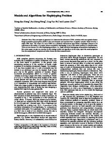
2.1.1. Morphology-based denoising and enhancement [6, 12] In MRA the vascular lumen usually appears brighter than the background, and can be visualized by means of the maximum intensity projection (MIP) technique. Ten years ago, when we initiated our first project in vascular image processing, MIP was the only widely available display mode capable of giving an overview of the vascularization. However, after projection the small low-intensity vessels disappear in noise, while their visualization is important, e.g. for the assessment of collateral vascularization of lower limbs in case of arterial obstruction. In order to denoise the dataset before the projection, while preserving the small vessels, we proposed a non-linear anisotropic filter composed of two stages. The first one is used to estimate the local orientation of the structures contained in the image and the second one performs the actual filtering along this orientation [6]. In order to estimate the orientation, a structuring element composed of a set of parallel line segments (sticks, see section 3.2.1) sweeps a number of discrete angles and the following criterion is evaluated for each angle φ: C(φ) = D − αH, where D is the average intensity difference between the central stick and its parallel neighbors, while H represents the directional homogeneity and is calculated as the average of intensity standard deviations within each stick. The filtering is performed according to the orientation φ that maximizes C(φ). We proposed a generic directional filter that can perform both denoising and enhancement weighted by appropriate parameters [12]. It computes a truncated mean values in each stick, then it combines them using the Laplacian-based scheme. The filter was clinically evaluated in its purely denoising version. It improved the contrast-to-noise ratio by a factor 2 on average. 2.1.2. Hessian-based enhancement (unpublished) The visualization of the coronary arteries in both MRA and CTA images is challenging, due to the vicinity of the heart cavities, as well as to the heart motion that hampers the elimination of non-vessel structures. Several filters based on directional second derivatives (see section 3.2.2) have been proposed in the past, in order to highlight the tubular structures (vessels) while attenuating the background [8, 9]. These filters use the eigenanalysis of the Hessian matrix. In a vessel the second derivatives are expected to be close to zero in the direction of the axis, and strongly negative in the plane perpendicular to this axis. Accordingly, the eigen-values (|λ1 | ≤ |λ2 | ≤ |λ3 |) of the Hessian H should meet the following conditions: λ3 ≈ λ2 0, the considered voxel can be discarded. Indeed, tr(H) = λ1 + λ2 + λ3 , det(H) = λ1 λ2 λ3 and the above-mentioned condition occurs only when one eigen-value is negative, while the remaining two are positive. When det(H) > 0 two other cases can be discarded by additionally computing the principal minors of H, in order to check whether or not H is definite positive with tr(H) > 0 (respectively definite negative with tr(H) < 0). As result, the computational time was further reduced by 25% on average. Now, a 200 × 200 × 80 voxels sub-volume containing the heart within a thoracic scan can be processed in one minute per scale on a Pentium IV, 1.7 GHz laptop. Figure 1 shows coronary arteries enhanced using our implementation of the Frangi’s filter [9]. 2.2. Pathway extraction for acquisition optimization, display and stenosis quantification The extraction of the axes of vascular segments has several applications. Knowing the local orientation of the vessels, optimal image acquisition quality can be achieved by an appropriate feedback onto the imaging device settings. The axis can be used to generate a virtual flight-through display or to compute the cross-sectional images essential both for visual evaluation of pathology severity and for more or less automated extraction of Machine GRAPHICS & VISION vol. , no. , pp.


5

measurements such as lumen diameters and areas, wall thickness, etc. These applications require that the axis orientation be consistent with the local orientation of the vessel. The axis extraction process is usually semi-automatic, since it starts from one or more seed-points interactively selected by the user. 2.2.1. Subtracted magnetic resonance angiography [19, 28, 29, 32] In the contrast-enhanced subtracted MRA the background is significantly darker than the vascular lumen, and the vascular pathway can be approximately determined by following the local maxima of the intensity. However, to achieve consistent orientations of the axis, we designed a method in which the continuity and smoothness of the axis are controlled by the elasticity and the flexibility of a model (see section 3.4) called extensible skeleton [19]. Starting from a user-selected point the skeleton grows by iteratively adding subsequent axis points within a prediction-estimation scheme (see section 4.1) controlled by a multi-scale analysis of the image moments (see section 3.2.3). The location of the next point is predicted according the local orientation of the tubular structure. The local orientation is estimated by calculating the eigen-vectors of the inertia matrix, where the intensities of the voxels play the role of elementary masses. The eigen-analysis is carried out at multiple scales, in order to cope with varying diameters of the vessel. The coordinates of the predicted point are corrected under the influence of image forces and of prior model shape constraints. Thus extracted axes were exploited to generate cross-sectional images in which an automatic boundary extraction was performed using adaptive iso-contours. The goal was a quantitative assessment of arterial stenoses, based on cross-sectional diameters and areas [28, 32]. The robustness and accuracy of the method have been evaluated on MRA data of 5 reference phantoms and of 17 patients’ carotid arteries. 97% of the centerlines were exploitable in the carotid arteries (100% in the phantoms). Mean difference (± standard deviation) between stenosis percentages semi-automatically measured and visually estimated by radiologists was 0.23% ± 7.89%. The reproducibility of the semi-automatic method was significantly better. Another application of the extracted axes is the optimization of the acquisition plane for blood flow measurement by phase contrast MRA. Accuracy of 2-dimensional imaging of blood flow depends on the alignment between the vessels and the imaging plane. This is challenging when the flow in several vessels is to be evaluated with one acquisition. The optimal plane is determined by minimizing misalignment between its normal vector and the axes’ tangent vectors [29]. The method was evaluated on a phantom and on 35 patients, by seeking the optimal plane for cerebral blood flow quantification simultaneously in internal carotids and vertebral arteries. In the phantom, difference of orientation and of height between known and calculated plane was 1.2 degrees and 2.5 mm respectively. In the patients, all but one axe were correctly extracted and the misalignment of the plane was within 12 degrees per artery. Machine GRAPHICS & VISION vol. , no. , pp.

6


2.2.2. Computed tomography angiography [26] Owing to bright structures (bones, calcifications) in CTA, the above-described method is not directly applicable. Based on an empirical study of the CTA image intensities, we proposed a pre-segmentation method using adaptive thresholding. The median axis of thus binarized image is then extracted. As this axis is expected to be located within the binary object, far from its boundaries, a 3D distance map is calculated. The axis is constructed by iteratively adding points corresponding to local maxima of the distance map. The iterative prediction/estimation scheme (see section 4.1) is similar to that described in section 2.2.1. Boundary location is refined by analyzing radial intensity profiles in the vicinity of their intersections with the thresholds (see section 3.1). The axis extraction was evaluated qualitatively in images of 60 patients. While using fixed thresholds only 50% of axes were exploitable, with adaptive thresholds 80% of previous failures were transformed into exploitable axes. The accuracy of boundary extraction was not rigorously assessed yet. 2.3. Quantification of lumen and wall in cross-sectional images While the focus of the projects described in sections 2.2.1 and 2.2.2 was the extraction of the axes, and the lumen contours were extracted by rather basic methods, the sections 2.3.1 and 2.3.2 report more advanced methods devised for the segmentation of both vascular lumen and wall. Recent evidence indicates that the type of atherosclerotic plaque, i.e. the composition and structure of the pathological vascular wall, rather than the degree of stenosis, is an important indicator of the risk of thromboembolic vascular events. It determines the plaque vulnerability to disruption. 2.3.1. High-resolution MRI of vascular wall [24] Depending on the antenna, acquisition sequence, strength of the magnetic field and other parameters, the resolution of MR images may fall below 0.1 mm. Such images are likely to provide evidence of the vessel wall composition. Although such resolutions are not yet available in clinical routine, several research groups anticipate the development of appropriate image processing tools. We addressed the problem of the extraction of the internal and external boundary of the vessel wall in high-resolution cross-sectional MR images as a preliminary step toward the analysis of the wall composition. We use an original implementation of active contours (see section 3.4.1) designed to permit an initialization with a single point. Its deformations are calculated on a normalized-length copy of the actual contour, which avoids costly re-discretization and re-computation of the inverse of the system matrix during the growth of the contour. The first contour is initialized by a point within the lumen. When its growth stops, the second contour is generated beyond the first (internal) boundary and grows until the external boundary of the vascular wall is reached. Machine GRAPHICS & VISION vol. , no. , pp.


7

Accuracy and reproducibility of this method were mainly assessed on high resolution MR images of rabbit aorta. Compared to contours traced by experts, the differences in endoluminal areas and in wall thickness were within the inter- and intra-variability of the experts, while the intra-variability of the method was significantly smaller. Ongoing work attempts to classify the components of the vessel wall, based on multi-spectral MR images, as well as on dynamic images obtained after administration of a contrast agent that progressively penetrates into some components of the wall. 2.3.2. Calcified CTA image analysis [35] The goal of one of our projects is the generation of patient-specific models of carotid arteries, for computational fluid dynamics simulations. We use CTA images in attempt to extract both wall thickness and calcifications, which is challenging due to current limitations of spatial resolution and of contrast in the vicinity of the vessel wall. However, the processing time does not need to be compatible with clinical routine and user intervention is allowed in order to provide an extra cue in the segmentation method. First, a search-ray scheme [30] is used to detect discontinuities (see section 3.1). From a point belonging to the lumen, a number of rays is cast and the radial intensity profiles are analyzed. Automatic differentiation between lumen and plaque is based on an empirical study of CTA image intensities [26]. At the end of this phase, each region is represented by a set of points defining a polygon. Then, the polygonal boundaries are refined, in order to improve continuity and to recover possibly missing parts, since in case of concave lumen some of its parts may be ”hidden” behind the calcifications. This is done by use of iso-contours. The adaptively calculated iso-values may be interactively adjusted at any moment, as the iso-contours are displayed in real time and the user can check their correctness. Lastly, iso-contours are also used to separate the inner and outer boundary of the wall. Pre-clinic evaluation of the method is ongoing. It can be noted however that, unlike the lumen and calcification boundaries, the semi-automatic extraction of the outer boundary is not based on image discontinuity evidence, but on radiologists’ experience. 2.4. Three-dimensional surface segmentation of cylinders While the extraction of the axis and of cross-sectional contours only provides measurements for conventional treatment planning and follow-up, the following two methods were devised to extract a complete surface of a given vessel, which is exploitable for the pre-operative simulation of the consequences of various therapeutic choices. They respectively use a discrete model and a continuous model of cylindrical surfaces. 2.4.1. Stent-pose planning [25, 37] Arterial stenoses and aneurysms are increasingly treated using stents (intravascular expandable grids). We attempted to facilitate the pre-operative choice of the stent’s length Machine GRAPHICS & VISION vol. , no. , pp.

8


and diameter by providing appropriate measurements and by interactively simulating the deployment of the stent within the segmented artery. An angiographic 3D image is first segmented using an active surface, actually a simplex mesh (see section 3.5.1), to create a patient-specific vascular model. A model of a folded stent is then slid along the vessel axis until an interactively chosen delivery location, and the model’s geometry is modified to simulate the unfolding of the stent. Lastly, the vessel model is re-meshed to fit the shape of the unfolded-stent model and thus to simulate the shape of the arterial lumen boundaries after stenting. The simulation is purely geometric and does not yet include mechanical interactions between the stent, the vessel wall and the surrounding tissues. Currently, both segmentation and simulation have only been visually evaluated. In general, the simulation is very useful to assess the positioning of the stent and if the stent diameter fits to the vessel’s healthy segments. However, the segmentation is sometimes inaccurate when two vessels are too close and cannot be distinguished because of an insufficient resolution of the images. In some cases we also noticed that the vessel axis is not well centered within the vessel lumen. This occurs when the vessel bends strongly. 2.4.2. Volumetric quantification of lumen in CTA [21, 33, 36, 38] This method is based on a parametric model of a generalized cylindrical surface [21](see section 3.5.2), using the state representation of systems. The model consists of an axis and of a surface obtained by continuously sliding, along the axis, a planar contour that remains locally perpendicular to it. Actually, the contour is represented in a reference frame, the origin of which slides along the axis, while one of its constituent vectors remains tangent to the axis. The state variables and matrices describe the evolution of this frame (location and orientation) and of the contour shape between the ends of the axis. Our method identifies the parameters of the model from a series of contours, using a Kalman state estimator (KSE). The method is initialized by computing an image of intensity gradient magnitude |∇(f (x))| and a line coarsely corresponding to the vessel pathway between a pair of seed points interactively chosen inside the vascular lumen. This line is obtained as follows: 1) a binary image is computed from the input dataset, using two adaptive thresholds (see section 2.2.2), 2) a distance map is calculated within thus extracted approximate vascular lumen, and 3) a minimum-cost path is computed between the seed points [20]. Then the KSE (see section 4.1) is used to sequentially control the extraction of planar contours in consecutive planes orthogonal to the approximate pathway, and to add cylinder pieces (comprised between each pair of contours) to the final model. The contours are described by a Fourier series (FS) decomposition, in which each harmonic of order n corresponds to an ellipse. Each cylinder piece is expected to have constant values of state variables, which is equivalent to locally constant axial curvature and torsion, constant rotation angle of the reference frame with respect to the Frenet frame, and linear variation of the FS coefficients. With constant axial curvature and torsion the axis piece is a helix. Using Machine GRAPHICS & VISION vol. , no. , pp.


9

Fig. 2. Cross-sectional lumen contours and whole cylinders reconstructed and superimposed onto the original datasets (rendered with shaded surface display). The bright spots are calcifications. The upper and lower cross-sections respectively correspond to the datasets on the left and on the right.

this property, an observation vector is calculated from two consecutive contours, i.e. the values of the state variables are deduced from the locations, orientations and shapes of these contours [33]. The observation is then filtered by the KSE to produce an estimate of the cylinder piece. The KSE adapts the progression speed to the complexity of the local vascular shapes (axial and superficial): in complex shapes (e.g. high local changes of curvature) the predicted length of the cylinder piece is automatically decreased, in order to reduce the difference between predictions and observations. The accuracy of the segmentation depends on the accuracy of the contour extraction. Furthermore, as numerous contours are to be extracted, the extraction method has to be fast. We have chosen the fast-marching implementation of the implicit deformable contours (see section 3.4.2). The contour is represented by a front that propagates outwards from the intersection point between the current plane and the curve representing the approximate pathway. Its displacement is driven by the Eikonal equation (see Eq. 17, section 4.2), in which F (x) is a monotonic propagation speed. This monotonicity leads to problems that we attempted to solve in our work [38]. We describe hereafter in details one of its variants that was only presented in a short poster [36]. • Speed function. Usual speed functions are exponential: F (x) = exp(−α|∇(f (x))|), or sigmoid: F (x) = 1 − 1/(1 + exp(−(|∇(f (x))| − α)/β)). However, these functions are Machine GRAPHICS & VISION vol. , no. , pp.

10


not appropriate when the contrast is strongly variable, like in vascular cross-sections with calcifications. Indeed, when the front reaches the low-contrast boundaries, it remains relatively far from the boundaries in the highly contrasted zones, and when it reaches the high-contrast boundaries, it already leaks far away through the lowcontrast breaches. Instead, we work with a ”brake” function B(x) = 1/F (x) obtained by multiplying the magnitude of the image intensity gradient by three exponential factors C(·): B(x) = |∇(f (x))|C(d(x), α1 , β1 )C(f (x), α2 , β2 )C(f (x), α3 , β3 ). The function C(·) of a scalar u is defined as follows: C(u, α, β) = 1 + exp(−(u − α)/β), where α is a shift and β is a signed sharpness parameter. In the first factor, d(x) is a mono-dimensional derivative of |∇(f (x))| in the normal direction with respect to the front, α1 = 0 and β1 > 0. In the remaining factors, α2 and α3 are respectively equal to the lower and upper limit of the typical range of luminal intensities in CTA images [26], β2 > 0 and β3 < 0. Thus, the front slows down not only for large values of |∇(f (x))|, but also after passing the discontinuity (d(x) < 0) and beyond the typical range of luminal intensities. • Stopping criterion. We want to detect the moment when the contour begins to ”leak” out of the lumen, so as to avoid wasting time for further propagation. The criterion is heuristic, based on experimental observations of the FS representation of the contours. The shape of a front propagating within the vascular lumen cross-section is initially circular, which can be represented by the fundamental harmonic alone (n = 1). The other harmonics (n > 1) increase slowly, as long as the front is confined within the lumen, but they ”explode” when the front begins to leak out of the lumen, since the shape becomes very irregular. At that moment, the standard deviations σn of these harmonics become larger than their mean values µn . We track the evolution of the harmonics up to the order 3, and the front propagation is stopped when both the 2nd and 3rd order harmonics meet the criterion: σn > µn . • Backtracking. With the above described modifications, we can expect that a front fitting to the actual vessel boundary exists and corresponds to a propagation time Topt slightly smaller than the stopping time Tstop . As all the front locations covered during the propagation are stored, we perform a backtracking, in order to select the front that maximizes the average gradient magnitude on its perimeter. If we note Ω(T ) the set of points x that compose the front at time T , and S(T ) = x∈Ω(T ) |∇(f (x))|, then: Topt = argmaxT {S(T )/card(Ω(T ))}. We evaluated the proposed method on CTA images representing 6 physical phantoms (having circular reference sections 6 mm in diameter, and two stenoses of variable shape, position, eccentricity and known severity) and on 76 CTA datasets representing the carotid arteries of patients (fig. 2). In the reference sections of the phantoms the mean error and standard deviation of the measured diameters were 0.14 mm ± 0.13 mm, while the stenosis percentage error was equal to 3.30% ± 5.06%. In the images of patients, the cylinders were visually inspected and scored from 0 (false) to 3 (perfect). 53 cylinders Machine GRAPHICS & VISION vol. , no. , pp.


11

obtained the score 3, 13 cylinders had perfect shape in healthy regions and some anomalies in diseased regions mainly owing to remaining difficulties to cope with calcifications, 10 cylinders were false, due to a bad shape of the initial minimal path, which occurs when the external carotid artery is locally ”stuck” to the internal carotid artery due to insufficient image resolution. The current implementation of the KSE, dependent on the initial approximate pathway, is responsible for this limitation. 2.5. Vascular tree segmentation The extraction of the vascular tree is helpful to remove the surrounding tissues and thus improve the display. It is also the first step toward an automated search of possible pathologies, in order to attract the attention of the physician and thus speed-up the analysis of huge datasets generated by modern scanners. The methods described in the following two sections focus on the skeleton of the vascular tree, while the volumetric segmentation is very rough. Both share the same framework, recursively extracting the branches (see section 4.1) by use of a spherical volume of interest (cell), which moves step-by-step along the vessels. At each step, the cell is initially centered in a predicted axis point. Its location and radius are iteratively modified, so as to encompass the vessel. The content of the cell is then segmented, in order to coarsely separate the vessel from the background. Then the connected components (CC) of the segmented sub-volume on the surface of the cell are analyzed. The number of CCs is interpreted as follows: 1 end of the branch, 2 - continuation of the current branch, 3 or more - bifurcation. New candidate points are predicted in consequence at the centers of the CCs, and the current center of the cell is added to a graph representing the vascular tree axes. Similarly, the segmented content of the cell is added to the union of the sub-volumes segmented in the previous iterations, so as to construct an approximate outline of the vascular lumen. 2.5.1. Well-contrasted images [27] By ”well-contrasted” we mean that the vessel can be coarsely separated from the surrounding tissues by thresholding (possibly adaptive and local, e.g. half the local maximum intensity in contrast-enhanced subtracted MRA). The adaptation of the cell size and position is based on the analysis of the surface CCs. Typically, at the beginning of its growth, the cell is contained within the vessel, so only one ”vessel” CC and zero ”background” CC is found. Then it begins to protrude from the vessel on one side, thus creating a ”background” CC. The location of the cell is then corrected by pushing its center in the opposite direction. The number of CCs may vary during the growth, until it stabilizes after a number of iterations, when the cell encompasses the vessel. Applied to 16 MRA images from patients, representing the neck (carotid, vertebral, basilar arteries, etc.) and the aorto-iliac region (with renal, mesenteric arteries, etc.), the method detected all the principal branches of the vascular tree and the bifurcations in which the secondary branch had at least 5% of the cross-sectional area compared to Machine GRAPHICS & VISION vol. , no. , pp.

12


the main branch. Some branches were not extracted owing to a strong local signal drop in severe stenoses. Conversely, a few false bifurcations have been detected, where two vessels were very close to each other and the assumption of good contrast did not hold. On average, the processing speed was 50 axis points per second. 2.5.2. Coronary arteries [34] In the datasets representing the coronary arteries, the surrounding structures may have both lower and higher intensities (respectively parenchyma and calcifications), as well as the same intensity range (heart ventricles filled with blood). Thresholding is therefore not applicable. Both the cell size adaptation and the detection of the vessel end are more difficult. To cope with these difficulties, we proposed two main innovations. • Thresholding is replaced by K-means clustering with an original metric. While the metric in the background cluster remains the intensity difference between the point and the mean value of this cluster, the metric of the foreground cluster is a combination of the intensity difference and the inertia moment with respect to the cluster’s principal inertia axis (see section 3.2.3) in the XYZ-space, weighted by a coefficient ϕ. This enforces the cylindrical shape of the segmented volume by including in the foreground cluster the voxels that are close to its axis even if their intensity sensibly differs from the mean intensity of the vessel, and by excluding the voxels that are located further from the axis even if they have similar intensity. In this way, we expect to separate the arteries of interest from other bright structures that appear ”stuck” to them in the images, such as veins or heart cavities. • The shape of the segmented sub-volume is checked against a geometric model (see section 3.3), in order to validate it as part of a vessel. Otherwise, i.e. when it is misshapen, we stop the extraction of the current branch. We also changed the implementation of the correction of the cell location and size. A distance map is calculated within the segmented volume and the position of this map’s maximum is used to update the candidate’s location if necessary. Then the ratio of the segmented volume to the total volume of the cell is compared with the theoretic ratio for a cylinder having a radius equal to half the radius of the cell. We increase or decrease the cell radius accordingly. The last step of the method is the local improvement of the axis. Since the cell must locally encompass the vessel and the predicted axis points are located on the cell surface, the distances between consecutive points are quite large. An advantage is a quick analysis of the vascular tree. A drawback however is that straight line segments joining two points are sometimes not entirely located within the segmented volume. To resolve this problem, a minimum cost path [20] is computed between the previous and current point, using a cost function based on the distance map. Thus calculated axis always lays within the vessel and closer to its center. The method is sensitive to the variation of the parameter ϕ. When its value is too small the adjacent structures are not eliminated, so the number of spurious branches is Machine GRAPHICS & VISION vol. , no. , pp.


13

higher. When the value is too high the bifurcations are considered as adjacent structures and they are eliminated. The missed branches may be recovered by use of additional seed points. On average, the processing speed was 1 axis point per second.

3. Models In medical image processing, underlying models are necessary to cope with incomplete, low-contrast and noisy data. This section gives an overview of the models used in the above-described methods. These models are classified according to increasing complexity. We begin with brightness patterns and simple geometric models useful (under some conditions) to identify points located either on the vessel boundary or on the vessel axis. Then we follow with active contours used to extract the cross-sectional boundaries. At the end, we describe complex models capable of representing a complete cylindrical shape. From now on, critical comments are provided for each model and algorithm.

3.1. Intensity profiles [26, 36, 35] The intensity profile is the simplest model, mainly used in the analysis of cross-sectional images. It consists of a straight-line segment (often called search ray) which can be manually traced by the user or generated in a ray casting scheme [30]. Depending on the algorithm, rays may have different line width and may be cast following different patterns (radial, spherical, cylindrical, normal to a more complex curve or surface, etc.), and the intensity values along the ray may be interpolated or smoothed. The profile models embed prior knowledge of intensities, contrasts and gradients, dependent on the imaging modality. In the methods described in sections 2.2.2 and 2.3.2 we used radial profiles, while in section 2.4.1 the rays were cast along the normal vectors from the nodes of the simplex surface mesh. In application to CTA images, these methods rely on the typical profiles experimentally determined in a previous study [26]. The main advantages of search ray based methods are the simplicity of implementation, the reduced computational time and the directional nature of the rays: the search rays can be defined according to the expected shape of the object, so that the image data be explored in an object-adapted way. However, several problems arise: 1) to interpret the profiles when the starting point of the rays is not guaranteed to lay within the vessel lumen and when their direction is not orthogonal to actual boundaries, 2) to manage the spatial continuity of the interfaces, 3) to reach certain parts of concave regions, when casting rays from one point, or 4) to avoid self-crossing of the rays cast orthogonally to an evolving complex interface. Nevertheless, this simple approach may be used to initialize a more sophisticated model. Machine GRAPHICS & VISION vol. , no. , pp.

14


3.2. Brightness patterns Almost all the existing methods in vascular image processing are based on the assumption that the vessel lumen is brighter than its neighborhood, which is consistent with the efforts done in the angiography imaging techniques. A few acquisition techniques however, particularly in MRA, provide ”black-blood” images. This can probably be overcome by a global inversion of the image dynamics. Nevertheless, in some cases this assumption is locally false, e.g.: in CTA images of the head, several arteries locally pass through holes in the skull and the bone is much brighter than the vessel (vascular wall is often too thin, compared with the image resolution, to give rise to a darker interface between the lumen and the bone). Similarly, concentric calcified atherosclerotic plaques, as well as stents, appear as direct neighborhood locally brighter than the lumen. These exceptions limit the application of the models described below. 3.2.1. Morphological model [6, 12] As mentioned in section 2.1.1, the model consists of 9 parallel line segments (sticks) of fixed length. If the sticks are aligned with a vessel, the longitudinal variation of intensity in each stick is expected to be small, while the difference between the central stick and its neighbors should be large. Let f¯k be the truncated mean intensity k=8 within the k-th stick (k = 0 corresponds to the central stick), and let f˜ = 8f¯0 − k=1 f¯k be the output of the enhancement filter. Ideally, if the respective mean intensities of the vessel and of the background are fV and fB , we should have f˜ = 8(fV −fB ) >> 0 when the central stick is aligned on a thin vessel, and f˜ = 0 when it is entirely contained in the background, which leads to vessel enhancement with background suppression. The optimal orientation is sought by an exhaustive exploration of the discrete space of possible solutions, i.e. by rotating the sticks in all possible discrete directions. According to our experience, this procedure leads to a good alignment of the model with the structures perceptible in the image: axes of small vessels and boundaries of larger objects. In the absence of such structures, the model aligns itself on random noise configurations. The main drawback of this model is an inevitably time-consuming implementation of the search of the optimal orientation. For this reason, although a multi-scale generalization would be straightforward (by use of sticks having variable length and spacing), only a mono-scale version is used, so that only small vessels can be enhanced. Furthermore, this model hardly fits the vessels with locally strong curvature. The model does not sufficiently distinguish ”line-like” structures from ”plate-like” structures and edges. Hence, while the background is well suppressed, thin objects and the edges of highly contrasted objects remain in the filtered image. 3.2.2. Second derivatives Another way of characterizing the intensity variations, small along the vessel and large in the cross-sectional plane, is the use of second derivatives (see section 2.1.2). Unlike Machine GRAPHICS & VISION vol. , no. , pp.

15


the above-described model, this approach does not require an exhaustive search of the optimal orientation, although such implementation has been proposed in the past [4]. Instead, the Hessian matrix is built with 6 partial derivatives that are usually computed by convolving the image with the appropriate derivatives of a Gaussian kernel, the standard deviation (σ) of which determines the scale (fxx = f ⊗ Gσxx , fxy = fyx = f ⊗ Gσxy , fxz = fzx = f ⊗ Gσxz , fyy = f ⊗ Gσyy , fyz = fzy = f ⊗ Gσyz and fzz = f ⊗ Gσzz ): 

fxx H =  fyx fzx

fxy fyy fzy

 fxz fyz  . fzz

(1)

Its eigen-vector associated with the eigen-value λ1 (having the smallest absolute value) determines the axial orientation. A ”vesselness” criterion is computed, based on the eigen-values, e.g. the Frangi’s criterion [9]: 2 2 f˜ = 1 − exp(−RA /2a2 ) exp(−RB /2b2 ) 1 − exp(−S 2 /2c2 ) ,

(2)

√ measures the cross-sectional circularity RA = |λ2 /λ3 |, axial elongation RB = |λ1 | / λ2 λ3 and local non-uniformity S = λ21 + λ22 + λ23 (a, b and c are weighting parameters). Since a computationally efficient implementation is possible (see section 2.1.2), multiscale analysis is used, and the optimal scale (with largest response of the filter) provides an estimate of the local vessel radius, which is an interesting feature. However, this model may locally be inappropriate, when singularities occur owing to stenoses and bifurcations. When implementing a ”vesselness” criterion, the choice of weighting parameters may be difficult, e.g.: in Frangi’s filter, while the parameters a and b may remain fixed, c depends on the image dynamics. Furthermore, strongly contrasted ”plate-like” objects often remain in the filtered image. 3.2.3. Inertia moments [19, 28, 32] In the method used in section 2.2.1, but also in [22], the underlying model is the so-called equivalent ellipsoid, i.e. elongated object that revolves with minimum inertia moment Ia around its principal axis a. Equations from mechanics are used with image intensities instead of mass density. The matrix of inertia: 

Ixx I =  Iyx Izx

Ixy Iyy Izy

 Ixz Iyz  Izz

(3)

with respect to a reference frame, the origin of which is the gravity center, is defined by the moments of inertia Ixx , Iyy , Izz with respect to the axes of the reference frame, and Machine GRAPHICS & VISION vol. , no. , pp.

16


by the products of inertia Ixy = Iyx , Ixz = Izx and Iyz = Izy : Ixx ≡ f (xj )(yj2 + zj2 ), Iyy ≡ f (xj )(zj2 + x2j ), xj ∈S(x,ρ) xj ∈S(x,ρ) Izz ≡ f (xj )(x2j + yj2 ), xj ∈S(x,ρ) f (xj )xj yj , Ixz ≡ − f (xj )xj zj , Ixy ≡ − xj ∈S(x,ρ) xj ∈S(x,ρ) Iyz ≡ − f (xj )yj zj ,

(4)

xj ∈S(x,ρ)

calculated within a spherical cell S(x, ρ) centered in x = (x, y, z) and with radius ρ. The moment of inertia with respect to a is: Ia = eTa I ea , where ea is the unit vector in the direction a. The orientation of a can be inferred from the eigen-analysis of I. Let λ1 ≤ λ2 ≤ λ3 denote the eigenvalues of I and e1 , e2 , e3 be the associated eigenvectors. Like in section 3.2.2, the axis orientation is given by e1 , while e2 and e3 define the orthogonal plane. When the cell contains a thin cylinder with a circular cross-section, then λ1