Models for extending streamflow data: a case study - CiteSeerX

Hydrological Sciences -Journal- des Sciences Hydrologiques,40,3, June 1995

Models for extending streamflow data: a case study H. RAMAN, S. MOHAN & P. PADALINATHAN Department of Civil Engineering, Indian Institute of Technology, Madras 600 036, India Abstract Models are proposed to extend the monthly streamflow data at a site where the available historic rainfall and streamflow data are too short for adequate systems study, subject to the condition that there are no gauging sites in the basin or adjacent basins with a longer period of streamflow data. Hence rainfall data of a nearby raingauge station are used. Five regression models, namely, runoff coefficient model, single linear regression, monthly linear regression, monthly linear regression with stochastic description for residuals, and a double regressed model are used. The results show that the monthly linear regression model with stochastic description for the residuals is best suited for the purpose when applied to a case study. Modèles d'extension de données de débits: une étude de cas Résumé Plusieurs modèles seront proposés dans ce papier en vue d'étendre une série de débits mensuels en un site où les données de pluies et de débits historiques sont trop courtes compte tenu de l'objectif poursuivi, ceci dans le cas où il n'existe pas, ni dans le bassin étudié ni dans un bassin adjacent, de site de jaugeage possédant une plus longue chronique de mesures de débits. Ce sont alors les données pluviométriques d'une station voisine qui seront utilisées. Cinq modèles régressifs, à savoir un modèle de coefficient d'écoulement, une régression linéaire simple, une régression linéaire mensuelle, une régression linéaire mensuelle avec modélisation stochastique des résidus et un modèle de double régression ont été utilisés. Il apparait, dans le cadre d'une étude de cas, que la régression linéaire mensuelle avec modélisation stochastique des résidus est le modèle le plus satisfaisant. INTRODUCTION Water resources systems are complex and need systematic study with reliable data to arrive at optimal planning and management decisions. In developing countries, the expansion of hydrological data collection networks often accompanies or lags development and planning rather than preceding it (Higgins, 1981). In Tamil Nadu State, India, utilization of surface water resources is almost complete and the focus has been shifted to evolve optimal management and operation of existing reservoirs. However, for some of the reservoirs (particularly small reservoirs) the streamflow records available are of very short duration. Also, these reservoirs lack details regarding catchment Open for discussion until 1 December 1995

381

382

H. Raman et al.

and related parameters. Reliable results from a systems study can be obtained only when streamflow data are available for a minimum period of about 35 years. Thus, it is necessary, given long rainfall records locally or from adjacent catchments, to estimate the streamflow hydrograph which would have corresponded to such a long hyetograph, termed as "extending" the streamflow record (Clarke, 1973). A detailed report on different conceptual and empirical rainfall-runoff models as applied to prediction and data extension is given by Clarke (1976). These models can be used for extending streamflow data. Conceptual models suggested by Dawdy & O'Donnell (1965) or Nash & Sutcliffe (1970) require a significant number of hydrological and meteorological parameters. Sittner (1976) has listed ten conceptual models and discussed in detail the application of these models. The application of wide ranging conceptual models for rainfall-runoff modelling is also reported by Singh (1981). Pitman (1978) studied four rainfall-runoff models of differing complexity and stated that the most complex model is not necessarily the best for all hydrological problems when data are sparse and non-representative. Diskin (1970) viewed a linear regression model as a simple conceptual model and explained the physical meaning of the regression coefficients. Loague & Freeze (1985) used regression, unit hydrograph and quasi-physically based models for upland catchments and concluded that regression models perform marginally better. Hamlin & Kottegoda (1971) extended the record of the River Teme using a bivariate model for generating synthetic overflow sequences. Higgins (1981) suggested an exponential decay function employed in a linear rainfall-runoff model for use in wet tropical catchments. This model cannot be used for extending data because it requires the ratio between long term runoff and rainfall. Driver & Troutman (1989) used linear regression models for estimating urban stormrunoff quantity and quality. Troutman (1985) discussed the errors and parameter estimation for regression models to be used in rainfall-runoff modelling in detail. Errors from these models are usually assumed to be: (i) statistically independent of each other; (ii) statistically independent of predictions; (iii) identically distributed; and (iv) normally distributed with mean zero and variance a^. He treated the regression models on a par with physically based models with the main focus on the minimization of error. The use of various regression models in data extension has been dealt with in detail by Hirsch (1979, 1982) and Hirsch & Gilroy (1984). The variance of the regression estimate is always biased downward since regression estimates lie on the regression line while the actual data are scattered about the regression line. Errors in the regression model are added as a noise component by Hirsch (1982) and this procedure affects the serial correlation structure of the record. A class of methods known as maintenance of variance extension (MOVE) suggested by Hirsch (1982) and various other procedures have been dealt with in detail by Alley & Burns (1983), Vogel & Stedinger (1985), Grygier et al. (1989), and Hirsch et al. (1993) in order to reduce the bias in the variance. All the studies referred to above use a base station with a long

Models for extending streamflow data

383

flow record for data extension. In this paper, an attempt has been made to extend the streamflow data in a sparse data environment. Various regression models were used and the errors in the regression models also modelled. These models were applied to the problem of extending the streamflow data at a flow gauging site (Site A) with limited rainfall and streamflow data with the provision that a long term rainfall record was available for a nearby station (Site B). Site A was the only gauging site in the study area. Further, no other meteorological data were available for the study at Site A or Site B. In this case, the following procedures could be used to extend the streamflow record: (a) using a suitable runoff coefficient to estimate the runoff from the rainfall data of Site B; (b) regressing the Site A runoff on Site B rainfall using an annual model or monthly models; (c) extending the rainfall record at Site A by regressing the rainfall at Site A on that at Site B and computing the runoff at Site A using a rainfallrunoff regression equation for Site A. The errors in the regression model are usually assumed as a noise component and are assumed to be normally distributed. The following model is suggested if the errors have a dependence structure; and (d) modelling the residuals of (b) using time series analysis and adding them to the model developed in (b). If the residuals are random, then they are to be added as a noise component. Model (d) may be used to maintain the variance of extended data, which usually tend downwards when a regression model is used for data extension. The models were applied to the Kudhiraiyar basin in Tamil Nadu, where eight years of rainfall and runoff data were available at the reservoir site along with rainfall data for 35 years at the nearby raingauge station, namely, Palani. The regression models were fitted using the method of least squares and evaluated using five numerical criteria in order to choose the best model. The selected model was validated for a period of one year and then used to extend the streamflow record for a period of 27 years.

STUDY AREA The water resource system chosen for the present study is the Kudhiraiyar Basin, a sub-basin of the Amaravathy River located in Tamil Nadu State, India (Fig. 1). The basin lies approximately between latitude 10°23'0"N and 10°42'30"N and longitude 77°22'30"E and 77°36'30"E. The Kudhiraiyar River originates from the Palani Shola hills and is 17.7 km long with a catchment area of 74.7 km2. The entire catchment is hilly and covered with dense forest. The basin area lies in a semiarid zone, subjected to the influence of the northeast monsoon. The average annual rainfall is about 700 mm. About 65 % of this rainfall is received during the months of September to December.

H. Raman et al.

Scale in km a b c d

Streamflow Gauging Station Kudhiraiyar Reservoir Kudhiraiyar Raingauge Station Palani Raingauge Station

Fig. 1 Basin Map of Kudhiraiyar.

The Kudhiraiyar reservoir was built during 1986-1988 and became operational in January 1989. A raingauge and a flow measuring device were installed near the reservoir site in 1984. Gauged daily flow and rainfall data are available from 1984-1991, a period of eight years. During the operation phase, the field engineers were unable to release water optimally and hence a detailed system study was undertaken for decision making regarding optimal releases and cropping pattern. Since the inflow data available was of shorter duration and there were no adjacent basins with longer flow data, extension of the flow record was envisaged. Monthly rainfall data for a nearby raingauge station, Palani, 15 km from the reservoir site, were used for this purpose. The monthly rainfall data were available for a period of 35 years from 1957-1991. The average annual rainfall at Palani is 738 mm. The value of the correlation coefficient between monthly rainfalls at Palani and Kudhiraiyar for the period 1984-1991 was found to be 0.837.

MODELS FOR EXTENDING STREAMFLOW DATA Runoff coefficient model (RCM) In the runoff coefficient model the runoff is related to the rainfall by a coefficient via: Q, = CPtA

(1)

Models for extending streamflow data

385

where Qt = monthly runoff volume (Mm3) in the period t; C = coefficient of runoff; Pt = monthly rainfall (m) in period t; and A = catchment area (km2), This is a very simple method and is usually used when no information is available about flows. Mohanakrishnan (1990) has derived and reported values of C to be adopted for south Indian river basins for various topographic conditions'. He suggested a value of 0.25 for the Amaravathy basin and that value was used in the present study.

Single regression model (SRM) between Palani rainfall and KudMraiyar flows In the single regression model, the monthly rainfall and runoff were related via: Q, = ao+avpt+et

(2)

where a0, ax = regression coefficients; Pt = monthly rainfall (mm) in period t; and Qt = runoff (Mm3) in period t. The monthly rainfall and runoff series were used to compute the coefficients. This did not account for the periodic nature of the series as it used the same coefficients for all months.

Monthly linear regression model (MLM) between Palani rainfall and KudMraiyar flows In the monthly linear model, the rainfall-runoff relationship was: Qi,t = atfi+at,vpi,t

+e

ij

t =

1,2,...,12

(3)

3

where Qt, = inflow (Mm ) in month t of year i; Pu = rainfall (mm) of month t and year i; and at 0, atl = regression coefficients for month t. This model has twelve equations, one for each month.

Monthly linear regression model with stochastic modelling of residuals (MLS) The residuals of the model given by equation (3) were tested for their independence and normality. If independent, then a noise component was added. If there was a dependence structure, then the autoregressive moving average (ARMA) class of models suggested by Box & Jenkins (1976) were fitted to the residuals of equation (3). The residuals were computed by: e

i,t

=

û/,/(actual) ~ ^M(reg)

^ '

The residuals when stochastically modelled for an ARMA(p, +e

H

Qi,t = ct,o + ct,vKi,t + ei,t

t=

1.2,..., 12

r = 1,2, ...,12

(7) (8)

where Kt t and P,, = rainfall in month t and year i of Kudhiraiyar and Palani respectively; bi0, biX = regression coefficients for Kudhiraiyar and Palani rainfall and ci0, ctl = regression coefficients for Kudhiraiyar rainfall and Kudhiraiyar runoff. The fitted models were evaluated based on the following five criteria: 1. Sum of squares of residuals (SOS) (Spiegel, 1972):

SOS = 2.

î(Qot-Qt)2

where Qot = computed flows and Qt = actual flows (Mm3). Coefficient of variation of residual error (CVR) (WMO, 1975):

(mî(Qot-Qt)2 CVR =

3.

l

±

* 100

where Qt = mean flow (Mm3) of month t, Ratio of absolute error to mean (RAM) (WMO, 1975):

Models for extending streamflow data

4.

387

l\Qot-Qt\ RAM = i^ , * 100 *Qt Mean Percentage Error (MPE) (Pindyck & Rubenfeld, 1981):

E(G«-fi,) MPE = 5.

'-±

* 100

Mean Absolute Percentage Error (MAPE) (Pindyck & Rubenfeld, 1981):

Elô«-e,i MAPE = ^1

* 100 nQt

APPLICATION The selected five models were applied to the data pertaining to the Kudhiraiyar basin. Of the eight years of available data, seven years were used for model application and calibration and the remaining one year of data used for validation. The single regression model was given by: Qt = 0.3204 +0.0073 Pt The standard error of the coefficient a was 0.000249 and the R value 0.755. The values of the regression coefficients for the monthly linear regression model are given in Table 1. The values of the constants and slopes of the regression equations were highly variable from month to month indicating that a single regression model may not fully serve the purpose. The slopes for all the months were positive and much higher than the standard error values except Table 1 Coefficients of monthly linear model Month

a

January February March April May June July August September October November December

0.5012 0.3651 0.2022 0.2115 0.2426 0.1137 0.1196 0.1782 0.1840 0.7157 0.2571 0.2480

l,0

Standard error is given within brackets.

«M

0.0098 (0.0008) 0.0010 (0.0025) 0.0052 (0.0017) 0.0019 (0.0005) ^0.0004 (0.0005) 0.0199 (0.0009) 0.0024(0.0011) 0.0219(0.0025) 0.0040 (0.0007) 0.0055 (0.0010) 0.0160(0.0015) 0.0301 (0.0023)

388

H. Raman et al.

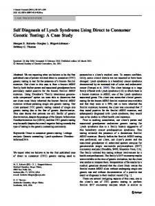
for the month of May which was negative and lower than the standard error, and hence insignificant. For the third model, the residuals of the above model were computed using equation (5). The normality of the residuals was checked using the skewness test of normality given in Salas et al. (1980). The limiting values of g at 90 and 95% confidence levels, for a sample length of 84 are given as 0.617 and 0.4228. As the value of g was 0.3429, the residual series was normally distributed. The autocorrelation function (ACF) and partial autocorrelation function (PACF) of the residuals are given in Fig. 2. From the figure, as the ACF and PACF values of the first lag were outside the confidence interval, it was evident that the series had a dependence structure that had to be modelled stochastically. Also it was evident from the ACF and PACF that AR(1), AR(2) and ARMA( 1,1) were the candidate models to be chosen for fitting the stochastic component. The final model parameters, white noise variance and the Akaike information criterion (AIC) for the candidate models (a) i 0.8

ACF

0.6 0.4 0.2 0 0.2 0.4 (b)

i 0.8 0.6 0.4 0.2 0 0.2 0.4

0

4

8

12 Lags (k)

16

20

Fig. 2 (a) ACF and (b) PACF of residuals of monthly linear regression model.

Models for extending streamflow data

389

Table 2 Stochastic model fitting for residuals of MLM