Division of Research and Technology and ... he research done in this area in Rutgers University. ... Table 8 Example of the LTPP Table MON-PROFILE-MASTER. Table 9 .... developing the models, since the information needed to be accurate.
FHWA-NJ-1999-030
Models for Pavement Deterioration Using LTPP FINAL REPORT October 2001 Submitted by Dr. Kaan Ozbay* Assistant Professor
Ryan Laub* Graduate Research Assistant
* Dept. of Civil & Environmental EIngineering Rutgers, The State University Piscataway, NJ 08854-8014
NJDOT Research Project Manager Mr. Nicholas Vitillo
~
~
~~
In cooperation with New Jersey Department of Transportation Division of Research and Technology and U.S. Department of Transportation Federal Highway Administration
Disclaimer Statement "The contents of this report reflect the views of the author(s) who is (are) responsible for the facts and the accuracy of the data presented herein. The contents do not necessarily reflect the official views or policies of the New Jersey Department of Transportation or the Federal Highway Administration. This report does not constitute a standard, specification, or regulation." The contents of this report reflect the views of the authors, who are responsible for the facts and the accuracy of the information presented herein. This document is disseminated under the sponsorship of the Department of Transportation, University Transportation Centers Program, in the interest of information exchange. The U.S. Government assumes no liability for the contents or use thereof.
1. Report No.
2 . Government Accession No.
3 . R e c i p i e n t ' s C a t a l o g No.
HWA-NJ- 1999-030 4 . Title and Subtitle
fi. Report Date
Oct 200 1
vlodels for Pavement Deterioration Using LTPP
15.
Performing Organization Code
Rutgers 7 . Author(s)
8. Performing Organization Report N o .
>r. Kaan Ozbay, Ryan Laub 9 . Performing Organization Name and Address
10. Work Unit No
New Jersey Department of Transportation CN 600 Trenton, NJ 08625
1 1 . Contract or Grant No.
. 1 3 . Type of Report and Period Covered 1 2 . Sponsoring Agency Name and Address
:ederal Highway Administration J.S. Deparhnen; of Transportation Washington. D.C.
I
Final Report 06/27/1997 - 03/31/1999 14. Soonsorine Aeencv Code
1 5 . Supplementary Notes
6. Abstract
4s pavement condition grows to be one of the crucial problems facing our national highway system, a new :hallenge emerges in developing pavement deterioration prediction models that are reliable yet easily applicable i y Highway Pavement Management System (HPMS) in State DOTS and other agencies. This reports presents he research done in this area in Rutgers University. The significant contribution of this research lies in the fact hat it utilizes the most comprehensive database of pavement conditions (LlTP) that is readily available and iromises to provide the sought data in future years. The Long Term Pavement Project (LTTP) Database jeveloped by the Federal Highway Administration was chosen to provide the required data of related parameters 'or the model development. The first part of this report reviews the existing literature covering related topics ncluding pavement roughness, the Long Term Pavement Project LTPP background, artificial neural networks, .egression analysis and the existing pavement deterioration models developed by Federal Highway Agency or .eported by Transportation Research Record as well as the default model that is utilized by the Pavement Management System. The second part discusses the work done in data analysis and data manipulation in addition to the development of the training of the neural network model. The third part deals with various aspects Df the model development using neural networks and regression analysis. The next part concludes the research Nith summarizing the results of model development and then by presenting a comparison between the models jeveloped in this research and some existing models by applying these models to similar data sets and Derforming statistical analysis of the results. Lastly, the report presents some recommendations for future -esearch in this area.
18. Distribution Statement
17 Key Words
Pavement Deterioration Models, Pavement Roughness, LTTP, Neural Networks, Pavement Management Systems 19. Security Classif (of this report)
Unclassified
20 Securitv Classif. (of this oaeel
I 148
Unclassified
? o m DOT F 1700.7 (8-69)
i
I
LIST OF FIGURES Figure 1 Research Methodology Figure 2 Representation of a Single Neuron in a NN Figure 3 Representation of a Multiple Layer NN Figure 4 Example of NN Training Program Written in Matlab Figure 5 Example of NN Program to Test the Trained NN Figure 6 Basic Flowchart for Backpropagation NN Algorithm Figure 7 Plot of the Default Pavement Deterioration Model Figure 8 Location of New Jersey GPS 1 and 2 Sites Figure 9 GPS Site with Irregular Trend Figure 10 Plot of Left and Right Wheel Paths Figure 11 Typical IRI Vs. Age Plot for Typical GPS 2 Site Figure 12 Flowchart for Determining the Optimal NN Architecture Figure 13 S.S.E. of NN with Respect to the Number of Node in the Hidden Layer Figure 14 Correlation of the Predicted IRI Vs. the Actual IRI Figure 15 S.S.E. of NN with Respect to the Number of Nodes Figure 16 Magnification of Figure 4-4a Figure 17 Results of the Lee Model Figure 18 Predicted Vs. Actual Roughness Using the Default HPMS Model Figure 19 Plot Of All Pavement Models Results Figure 20 Plot of Actual IRI Vs. Predicted IRI for 1-78 Figure 21 Plot of Actual IRI Vs. Predicted IRI for 1-80 (Asphalt on Asphalt) Figure 22 Plot of Actual IRI Vs. Predicted IRI for 1-80 (Asphalt on Concrete) Figure 23 Summary of Model RMSE
Page 3 11 12 13 14 16 23 25 31 33 38 53 54 55 56 56 82 83 88 93 94 95 98
LIST OF TABLES Pane Table 1 Description of the General Pavement Studies Table 2 Summary Of The IMS Database Modules Table 3 Results of the Example Neural Network Training Table 4 Summary of FHWA Model Parameters for GPS 2 Pavements Table 5 GPS Sites Requested in Wet Freeze Zones Table 6 Example of the LTPP Table EXPERIMENT-SECTION Table 7 Example of the LTPP Table INV-AGE Table 8 Example of the LTPP Table MON-PROFILE-MASTER Table 9 Example of the LTPP Table TRF-EST-ANL-TOT-LTPP-LN Table 10 Data from a Typical GPS 2 Site Table 11 Description of Sub-Model Variables Table 12 Summary of Sub-Model Variables Table 13 Stepwise Regression Table 14 Standard Linear Regression Table 15 T-Values for the Standard Linear Regression Table 16 Linear Regression Sub-Model Testing Results Table 17 Sum Squared Errors for the Test Results of Table 4-6 Table 18 Sum Squared Error for Different Number of Nodes Table 19 Sum Squared Error as Hidden Layers Increase Table 20 Optimized Sum Squared Error as Hidden Layers Increase Table 21 Optimized Configuration of the NN Sub-Models Table 22 NN Model Predictions for Their Respective Test Points Table 23 Sum Squared Error for Results Presented in Table 4-12 Table 24 NN Model Predicted Results Using Additional Data Table 25 Sum Squared Error for Results in Table 4-14 Table 26 Linear Regression Sub-Model Results with Additional Data Table 27 Sum Squared Error for Results of Table 4-16 Table 28 Testing Results of GRNN Estimates Using the Test Data Table 29 Weights for the Input Layers of the RITS NN Model Table 30 Bias for all the Layers of the RlTS NN Model Table 31 Weights for the Hidden Layer of the RlTS NN Model Table 32 Weights for the Output Layer of the RlTS NN Model Table 33 Excel Implementation of NN Calculations Table 34 Data Retrieved from LTPP Database for the FHWA Model Table 35 Partial Data Used for Validation of the FHWA Model Table 36 Data Used for Validation of the FHWA Model Table 37 Testing Results of the FHWA Model Table 38 Comparison on Sum Squared Errors of Both Models Table 39 PSR Predicted for the Eleven Test Points Table 40 IRI Converted from PSR Values in Table 6-4 Table 41 Sum Squared Error for the Lee Model Table 42 Testing Results of the Default HPMS Model Table 43 Summarized Test Results of All the Models
iii
7 8 15 20 26 28 29 30 36 41 44 46 47 47 47 49 50 54 56 57 57 58 59 61 62 64 65 67 68 69 69 69 72 75 75 76 77 78 80 80 81 84 86
Table 44 Squared Error for All the Models for the Test Data Table 45 Deviation of Initial IRI in New Pavements in New Jersey Table 46 Summary of RMSE
iv
87 91
96
TABLE OF CONTENTS
Paae INTRODUCTION Objective and Scope Methodology
1 2 2
LITERATURE REVIEW Review of Pavement Roughness Long Term Pavement Project (LTPP) Background Background on Neural Networks Review of Regression Analysis Existing Pavement Models FHWA Models Transportation Research Record Default Pavement Management Svstem Model
4 4 6 9 17 19 19 21 22
BUILDING A NEURAL NETWORK TRAINING DATABASE Choosing The Sites Data Manipulation Choosing The Variable Dejermination of StatisticaI sianificance Initial IRIS and Delta Variables Development of a Training Database For Neural Networks
24 24 27 37 37 39 42
MODEL DEVELOPMENT AND RESULTS Model Development Linear Regression Models Neural Networks Determininq the Optimal Number of Lavers and Nodes in the NN Summary of NN Results Results of The Sub-Models Additional Data General Regression Neural Networks
43 43 46 51
V
51 57 60 60 66
RUTGERS’ MODELS Rutgers’ Models
Pane 68 68
PAVEMENT DETERIORATION MODELS FHWA Model Model by Ying-Haur Lee Default Pavement Management System Model Conclusion
73 73 79 82 85
MODELS IN PAVEMENT MANAGEMENT SYSTEMS New Jersey Pavement Management System Data Initial IRI or IRI Indices Results Using NJDOT Pavement Management Data Summary of Results
89 89 89 92 97
FUTURE RESEARCH
99
APPENDIX A: IMS DATABASE FIELD DESCRIPTIONS APPENDIX B: TRAINING DATABASES DEVELOPED FROM LTPP DATA APPENDIX C: NN PROGRAMS, WEIGHT AND BIASES APPENDIX D: NJDOT PAVEMENT DATA FOR SITES USED IN STUDY
100 106 112 126
REFERENCES
139
vi
INTRODUCTION
There are thousands of miles of paved roads in the United States that are traveled daily by millions of cars and trucks transporting people and goods. For this reason, the condition of the Nation's roadways plays a very important role in everyday life. The importance of the quality of roadways is also clear to the federal government. Billions of dollars are spent to build, maintain, and improve roadways. The cost of building a new roadway or rehabilitating an existing pavement can be considerable. If these roads are not repaired, poor pavement conditions can be just as costly to the driving public. Rough pavements can decrease speeds of traffic flow, cause damage to vehicles, and increase the number of traffic accidents. These costs, defined as social costs, are difficult to quantify and unfortunately, are born by the public at large. To address these concerns, the Federal Highway Administration has developed guidelines for developing a Pavement System.(I)Many State Departments of Transportation (DOT) have developed to manage their highways. Being able to know when a pavement needs to be repaired before the pavement actually fails is an important element of management. Development of reliable pavement deterioration prediction models is a challenge to developers. Accurate pavement deterioration prediction models can be a valuable tool to the DOTSto achieve a more efficient highway management. Due to the challenges of modeling the behavior of pavements, current pavement management's strength depends upon the measurement of existing pavement conditions rather than predicting future conditions of pavements. Projected roughness trends are a big factor used for evaluation, since pavement roughness is a good indicator of its future performance. There is also the need for modeling different types of pavements. Portland cement concrete pavements are solid structures (i.e. rigid pavements). Most deterioration models for these structures are fairly accurate because their failure follows a more typical structural pattern. On the other hand, the deterioration of asphalt pavements is more difficult to predict due to the visco-elastic characteristic of the asphalt. Even though modeling the behavior of asphalt material can be easily done in a pavement laboratory, there are various external conditions that can be impossible to mimic. By including the many variables a roadway pavement endures, such as construction techniques, weathering or aging, the modeling effort becomes even more difficult.
1
OBJECTIVE AND SCOPE The objective of this report is to explain the research done at Rutgers University in the area of developing models that can predict pavement deterioration more accurately. Neural networks and linear regression are the tools selected for developing these models. Neural networks are capable of distinguishing trends in data that are not easily recognized by standard statistical techniques. Careful consideration was given to the data used in developing the models, since the information needed to be accurate. The Long Term Pavement Project Database developed by the Federal Highway Administration had the potentials of representing the type of data sought. This program has been collecting data since 1989 at hundreds of sites across North America. The LlTP database gathers data coveting a wide-range of variables and employs precise techniques for the collection of the information. These factors make this database an excellent choice for use in developing pavement models. The scope of research focuses on modeling one particular type of pavement from this database, specifically an asphalt pavement that consists only of its original structure (i.e. the pavement was never rehabilitated). The reason for choosing this type of pavement is that it represents the most basic type of asphalt pavement. All other types of asphalt pavement use this pavement as a foundation. Thus, any model developed in this research could be used as the basis for developing other pavement models. METHODOLOGY
Figure 1 represents the flow chart of the research methodology followed in this project. Multiple processes, shown in this Figure, are at times accomplished simultaneously. The first area of investigation is surveying the existing information on pavement deterioration models, pavement theory, regression analysis, and neural networks. In addition to the information on pavements, the LTPP database is investigated thoroughly. As a first step, a search of the database is performed for the sites that should be included for developing the models. After acquiring the requested data for these sites, further inspection of the available data is done. Statistical analysis of the data played an important role in the selection of the variables for the development of models. Once the variables are chosen for developing the models, they are compiled into a database. The neural network and linear regression models are then developed using the compiled database. A comparison of these models with some of the existing models is carried out afterwards.
2
Literature review of pavement deterioration models, pavement theory and
I
1
Investigation of the type of data available-
.t
]
Statistical analysis of data
Selection of relevant pavement variables to be used as inputs for the construction of NN models to predict IRI.
-+ I
I
I v
develop models. I
I
Construction of a database of the variables, for all relevant sites and compilation of all the data that will be used to train the NN
4
4 Development of linear regression models using the exact same data used to train the
Testing of the NN and linear regression models with data not used in the development of the models
I
Conclusions
I
Figure 1. Research Methodology
3
I ! Identify existing pavement deterioration Models
LITERATURE REVIEW This section presents a summary of the literature review that was done for the purpose of pavement model development. Pavement theory in general was studied, specifically pavement properties and mechanics. Emphasis was placed on pavement roughness, its measurement, existing indices and their correlation. Prospect tools for model development were also reviewed, mainly Neural Networks and Linear Regression. Their application, precision indicators and their statistical significance were studied thoroughly. L l T P background, data collection, database structure and its accessibility was also examined. Finally, extensive research for existing pavement models was performed by focusing on their input variables, validity and outcome reliability.
REVIEW OF PAVEMENT ROUGHNESS One of the main objectives of our transportation system is to provide a comfortable ride for users. Roadway roughness is a good indicator of whether this criteria will be fulfilled. A brief look at the historical development of this indicator can be useful. In the 1940’s the roadway longitudinal profiles were measured using an idmile scale, which was the popular basic unit of measurement.@)The inlmile scale represents the change in elevation over a given interval. In the ~ O ’ S the , devices used were simple and not as sophisticated and efficient as those used in recent years. There are many reasons why these devices did not measure the true profile of the roadway. One main reason was that the technology was not available to give a continuous reading of the roadway profiles. Another reason is that a vertical drop caused by a crack or a joint in the pavement gave an infinite change in the slope and made calculations difficult, if not impossible. To overcome this problem, data was collected in intervals of a fixed length. The early devices were one foot long sticks that were moved end over end. The difference in height of the ends of the sticks was recorded and converted into the in/mile units. Later devices that could measure the response of springs in a vehicle’s suspension were used to measure the roadway roughness by recording the response of those springs as it traveled along a road. There are many different devices that have been developed to measure roughness or ride quality. The main problem with these devices is that they do not employ a common standard. The different devices did not give results that could be compared to one another even for the same pavement. In the 1 9 7 0 ’ ~ the ~ NCHRP studied these different systems to better understand these problems by developing and testing mathematical models to demonstrate the response of vehicles to the roadway. The most famous model that came out of that NCHRP study was the quarter car model. In this algorithm, the behavior of one wheel of a car is modeled, including the effects of the suspension spring and damper. Including these effects was important because most road roughness was measured based on a response-type measuring system. This model demonstrates how a vehicle or a passenger is affected by the roughness of the road. One
4
major factor in why roughness measurements were not compatible or comparable was that the suspension of vehicles was not calibrated or standardized. Using accelerometers, computers, and the quarter car algorithms, a “virtual response-type system” can be developed.(’) This system can then be used to model the response of a vehicle to a pavement, or use a vehicle to measure the roughness of a pavement. Inaccurate and incompatible road roughness measurements were not experienced just in the United States. The findings of many World Bank sponsored research programs concluded that poor roads are costly to many developing countries. The cost of repair or reconstruction of pavements is high but the user costs as a result of rough roadways is even higher when calculated over the service life of the pavement. Road roughness indices were a primary factor for investigating the trade-off between the costs. This problem was the same as the one faced earlier in the United States because many countries used different roughness indices and standards. The roughness indices in reports submitted to the World Bank were suspect because they were measured by different standards and methods.(’) To provide a common quantitative basis on which the different measurement of roughness can be compared, the International Roughness Index (IRI) was developed at the International Road Roughness Experiment held in Brazil in 1982 under the sponsorship of the World Bank. The IRI summarizes the longitudinal surface profile in the wheelpath and is computed from the surface elevation data collected by either a topographic survey or a mechanical profilometer. It is defined by the average rectified slope (ARS), which is the ratio of the accumulated suspension motion to the distance traveled obtained from the mathematical model of a standard quarter car transversing a measured profile at a speed of 50 mph (80 km/h). It is expressed in units of inches per mile (m/km). One drawback to the IRI is that there exist an infinite number of profiles for a given roadway. A profile is a line along the path of a pavement with no width. Thus, theoretically, an infinite number of profiles exist for each roadway width. The vehicle used in the recording of the IRI will not travel in a perfectly straight line, and could produce a variance in the roughness measured. Procedures exist to compensate for this variability. Each time a profile was recorded, five profile runs were performed so that during each run, the profiles were within a given deviation of the normal (2% deviation) for all the runs. In the next section on building a neural network database, table 6-7 shows a minimum of five runs for each profile date. If one of these runs is not within the 2% deviation then additional runs are preformed. Those that are not within the 2% deviation are removed, and are not included in the database. In the LTPP database each profile run is recorded in the table MON-PROFILE-MASTER. The runs are in numerical sequence and so a profile run is not to be included if a break in the numerical sequence (i.e. 1, 2, 3, 5, 6) would occur. Several models in the reports reviewed used different types of measurementsfor roughness and deterioration. Although there is a considerable push for all State agencies to use the same indicators, this has not yet happened, thus reports that study the correlation between different pavement performance indices were investigated. IRI is the roughness indicator used in the LTPP database. For this reason, papers regarding the relationship of IRI and other roughness indicators were closely reviewed. A Transportation Road Research paper showing the relationship between PSR and IRI was used extensively for this project.(’’) The
5
document from ITX Stanley was more involved('g)as it includes relationships between several different types of roughness indices. Many of these relationships also involved IRI and RQI.
LONG TERM PAVEMENT PROJECT (LTPP)
In the 1987 Highway Act, congress authorized the strategic ,Highway Research Program (SHRP) which was a 5-year, $150 million research program. SHRP concentrated on asphalt, concrete, highway operations and structures, and pavement performance research results. The Long Term Pavement Project (LTPP) was originally designed as a twenty-year project to monitor and gather data on various types of pavements. After the first 5 years of data collection, SHRP had concluded its requirements as set by Congress. The remaining 15 years of the LTPP program was to be managed by the Eederal Highway Administration (FHWA). The FHWA is the current coordinator of the LTPP project and database. The objectives of the LTPP program were the following :(*'I Evaluate existing design methods. 0
0
0
Develop improved design methodologies and strategies for rehabilitation of existing pavements Develop improved design equations for new and reconstructed pavements. Determine the effects of (a) loading, (b) environment, (c) material properties and variability, (d) construction quality, and (e) maintenance level on pavement distress and performance. Establish a national long-term pavement database to support SHRP objectives and future needs.
The LTPP program was originally designed to include three types of studies: General Pavement Studies (GPS), Specific Pavement Studies (SPS), and Accelerated pavement Testing (APT). The largest of these studies is the GPS, and includes 742 in-service sections throughout the United States and Canada. The SPS have specific goals, and are performed by experimental approaches to achieve these goals. The APT has not yet been incorporated into the LTPP database. The GPS experiments within the LTPP program include the types described in table 1. It also includes the number of sites used in each GPS study. The LTPP project has been in existence for ten years with 7 to 8 years of the data processed and available for use. With more data from future years, any model developed with the first half of the data can be tested, refined and calibrated with the second half of the data.
6
Table 1. Description of the General Pavement Studies General Pavement Studies (GPS) Descriptions
I
GPS 1
I 1 I
GPS 2 GPS 3 GPS 4 GPS 5
I
Number of GPS Study Sites
Asphalt Concrete (AC) on Granular Base
191
AC on Bound Base
115
Jointed Plain Concrete
128 52
Jointed Reinforced Concrete ~~
Continuously Reinforced Concrete
75
GPS 6A
Existing AC Overlay on AC Pavement
51
GPS 6B
New AC Overlay on AC Pavement
57
GPS 7A
Existing AC Overlay on Portland Cement Concrete (PCC) Pavements
22
New AC overlay on PCC Pavements
24
Unbonded PCC Overlays on PCC Pavements
27
~
GPS 7B GPS 9
1
I
The data collected for the LTPP project is stored in the LTPP jnformation Management There are two components that control the data entry in the IMS database, the four regional offices and the central IMS office. The four regional offices focus on the data collection and the submitting of that data to the central office. Another requirement is to exercise quality control of regional personnel and control data collected and submitted by State Highway Agencies (SHAs). The central office is responsible for the climatic data, suality assurance (QA) of all LTPP data, and providing data to the public. The LTPP IMS has seven data modules, which contain the data collected from each GPS site. The modules as shown in table 2 categorize the data. The background information for each site is the most important information contained within these modules.
System (IMS).
The Inventory Module contains the historical information for each site in the database. The state departments of transportation generally provide this information. This data includes the location of the section, pavement type, layer thickness, layer type, material pro erties, composition, construction improvements, and other background information.(*' These records might not be always complete.
P
7
Table 2. Summary of IMS Database Modules
Sub-module
Number of Tables within Module
Inventory
None
26
Material Testing
None
76
Climate
None
5
Maintenance
None
9
Rehabilitation
None
49
Traffic
None
6
Automated and manual distress
8
Friction
1
Longitudinal Profile
2
Cross Profile
4
Deflection (FWD)
8
Module
Monitoring
Even though some material properties are given in the inventory record, material testing was also separately performed for this study. The information gathered from field sampling and laboratory material testing is contained in the Material Testing Module. This data verifies and documents the existing pavement structure for each site in the LTPP study. It also gives an evaluation of existing layers of the pavement. The laboratory testing involves over 40 different types of procedures, many of them are employed currently in designing pavement.(20) The climate data for a site is available in the Climate Module. This module shows the conditions recorded from at least one nearby weather station. Statistical estimates based on as many as five weather stations are also included. A summary of daily measurements, monthly statistics, and yearly average can be found for some of the sites. (20) Maintenance and rehabilitation is contained in their respective modules: Maintenance Module and Rehabilitation Module. The primary purpose of the Maintenance Module is to record all the activities relating to maintenance that was performed at the GPS site. This could include seal coating, patching, joint resealing, milling, or grooving. The Rehabilitation Module on the other hand includes any major improvement at a GPS site. Rehabilitation includes resurfacing, reconstruction, or addition of lanes. Anything that would have altered
8
the structure of a pavement is considered rehabilitation and its data is recorded in this module. The Trafic Module contains data regarding the annual traffic statistics for all the GPS sites. Counts by vehicle classification, and distributions of axle weights are some of the traffic factors in this module. The annual average daily traffic (AADT) statistic in the database applies only to one lane at each site. Traffic statistics in this section are based on monitored data, for approximately two-thirds of the sites. The remaining is based on historical records or is not included at all. The last module contains information on all the data gathered on the current conditions of the pavement at a site. The Monitoring Module contains several sub-modules; automated and manual distress, longitudinal profile, cross profile, and falling weight deflectometer. The Automated and Manual Distress section contains information regarding the pavement conditions. This concentrates primarily on the severity of surface defects. The Friction section of monitoring stores the friction number, surface type, test methods and other fields relating to the surface friction of the GPS sites. The Longitudinal Profile section contains the information on the longitudinal profile which is predominately measured in IRI. The Cross Profile section contains information regarding the transverse profile, commonly referred to as rut data. The last section of the Monitoring Module is called Falling-Weight Deflectometer. A falling-weight deflectometer measures the response of dynamic loads applied to a pavement structure. This loading and the data recorded from this test can determine the strength of the pavement along with the structure of the pavement. (20) This is an overview of the data contained in the LTPP database. There are many tables of varying length and width. It is difficult to image the full size of the overall database. Table 2 includes the number of table that are within each module. Chapter 3 of this report includes some examples of the table included in the LTPP database, which will give a better understanding of its large size.
Backgroundon Neural Networks Man has been interested in the workings of the human brain since the beginning of civilization. Many have tried to model its functions. Ancient Greek philosophers tried to conceptualize the thought process into mathematical formulae. This type of thinking has evolved with the aid of more powerful tools, like computers, which can now model the simple learning patterns of the brain. In the past few decades better understanding of the human process of intelligence has lead to its modeling on a computer. This is how neural networks, or rather artificial neural networks (ANN) come into play. An ANN attempts to model how the brain transmits information to the body. Major projects, which involved ANN, were performed in the 1960’s. One such project was called The Percep!ion, which was a mixture of neural networks and pre-processing algorithms. The Perception was based on the first stages of primitive vision based on
9
pattern recognition. This program could determine the gender of a person by ‘seeing’ hidher face. Research continued in the 70’s but it was not until the mid-80’s that wide spread interest in ANN grew with the proliferation of the computer itself. Now ANNs are used in a wide variety of research fields. An ANN acts as a biological neural network, that is, it acts as a network of neurons processing information. A single neuron is a single nerve cell and a chain of neurons transfers information to or from the brain. Neurons upon receiving information must interpret the information and determine what to do with it. A neuron could either pass information on to the next cell or it could cause a muscle to contract. The type of information passed on to other cells is dependent on past experiences. That is an infant does not know what pain feels like until it experiences it for the first time. An ANN works in the same way. Information put into an ANN is just like a signal from the braiin or nerve ending in a biological neural network. The individual signals in an ANN are called vectors, pin figure 2 or X in figure 3. What happens is that a set of inputs are applied to a network, which are labeled X1, X2, .... , X, in figure 3 . Each signal is then multiplied by an associated weight, W11, W21...Wnn, and then they are passed to the summation block in which they are summed. Each neuron outputs a weighted sum of the inputs. In this case it is a simple matrix multiplication. The example shown in figure 3 is used as an educational tool to understand the basic network structure. One example of this is called an activation function. Example: OUT= 1
if Yn > Z
OUT= 0
if Y n s Z
10
Inputs
General Neuron
a = m P + b)
Figure 2. Representationof a single neuron in a neural network
11
t
12
This is commonly used in visual recognition, in which the network will tell you if it is or is not the target sought. This is a linear activation function, but there can be non-linear activation functions too. Figure 2 represents a single neuron within a network. The variables in the diagram are as follows: P = all inputs vectors
W= weight applied to the inputs b = bias applied to the inputs
n = net input vector a = the final values once all the weights and biases are applied.
A neural network consists of many neurons combined together. The diagram in Figure 3 represents a multiple layer network consisting of nine neurons in three different layers. This network has architecture similar to the one in the program shown in Figure 4. Multilayer networks are more complex than single layer networks, and offer a greater ability for the computational capabilities than a single layer network. This layering mimics portions of the brain by using different algorithms. In the past decade algorithms were perfected and refined in order to train ANN with multiple layers. Figure 4 is a simple example of a NN training program written in Matlab. This program trains the NN to predict the simple equation:
Y=2X+5
P={12345678910}; T = { 7 9 11 13 15 17 19 21 23 25}; net = newff ([0 101, [ 4 1 11, { 'logsig' 'tansig' 'purelin'1 ) ; net.trainPararn.goa1 = le-100; net.trainParam.epochs = 500; net.trainParam.rnu = .01;
net.trainParam.mu-inc
=
net.trainParam.mu-dec net.trainParam.mu-rnax net = train (net,P,T) ;
.5; le90;
= =
10;
Figure 4. Example of NN Training Program Written in Matlab Using Matlab NN Toolbox (3)
13
1
D = t 1 . 5 2.5 3.5 4.5 5.5 6.5 7.5 8.5 9 . 5 } ; [R] = sim(net,D); V = (R)
Figure 5. Example of NN Program To Test The Trained Neural Networks
In figure 4, P represents the training input vectors for the NN, to predict equation [I]. Values within the brackets represents one set of input vectors. These values would correspond to the values in equation [I].
{w
The T represents the target vectors that the trained NN produces. In this case these values represent the {ZX + 5) portion of equation [I]. NEWFF is a function that performs a backpropagation NN training algorithm as part of the Matlab program. The brackets following it represent the input ranges and the NN architecture. A value representing the input range must be given in the training program. Since this is only a test this value will range from zero to ten, {P = 1,2...lo}. The [4 1 13 is the architecture of the NN program in figure 4. According to this NN architecture first layer has four nodes, the second layer has one nodes and the last (output layer) has one node. TANSIG represents the transfer function between the layers. This means that the output between the first layer and the second is transformed by a hyperbolic tangent sigmoid function. This function maps a neuron input from an interval of (-00 , +00 ) into an interval of (-1, +I). There are three different types of transfer functions in the Matlab NN toolbox: TANSIG, LOGSIG, and PURELIN. LOGSIG is a Log-Sigmoid transfer function, which fits the inputs into an interval of (0, +I). The PURLIN is the simplest of the transfer functions because it is simply a linear transformation of the input. The rest of the lines of the program are different training parameters. These parameters can be changed and adjusted. For example ...GOAL = 1E-I00 means that the NN will train until the mean square error (MSE) is under 1E -100. This is only one criteria that the Droaram uses to termiwte training. The MSE was chosen to be this low so that other limitations like the numbers of training epochs (net.trainParam.epochs = 500) could be reached. 500 epochs mean t'iat the NN will use the input data 500 times before terminating the training, unless another criteria for ending the training has been met. (3) To test how w t I the NN predicts equation [I], the program in figure 5 is run. This program contains nine t - j t points. These test points are, {1.5, 2.5, 3.5,4.5, 5.5, 6.5, 7.5, 8.5, 9.5}, and are shown as the D values. These are nine different points that were not used to train the NN. Table 3 shows the results of using these test points compared to the actual data.
14
Table 3. Results of example NN training
Y
2X + 5
NN prediction
% Difference
1.5
8
7.65
-4.38
2.5
10
10.16
1.64
3.5
12
11.89
-0.88
4.5
14
14.05
0.36
I 5.5 I
16
I
15.99
I
-0.06
I7.98
I 1 9.5
24
I
20.00