Aug 13, 2007 - Although wildlife can travel in either direction along the position axis .... Solving for qt requires knowledge of the unknown q. If q were known, ...
Models of Random Wildlife Movement with an Application to Distance Sampling1 Francis J. DiTraglia University of St Andrews Mathematical Institute
Supervisor: Len Thomas August 13, 2007
1
The author wishes to thank Steve Buckland, Rachel Fewster, Peter Jupp, and Clare Parnell for their many helpful comments and suggestions.
Abstract In this paper we present three models of random wildlife movement: a onedimensional model of wildlife-observer encounters on roads, an analogous twodimensional model, and an further two-dimensional model that borrows from the ideas of statistical mechanics. We then derive unbiased estimates of wildlife density in terms of encounters for each of these models. By extending these results to incorporate uncertain detection, we suggest three novel distance sampling methods and briefly consider possible field applications.
Contents 1 Introduction
2
2 Encounters in One Dimension
4
2.1
A Simple model of Encounters . . . . . . . . . . . . . . . . . . .
5
2.2
Observer Field of Vision . . . . . . . . . . . . . . . . . . . . . . .
12
2.3
A Generalized Model of Encounters . . . . . . . . . . . . . . . . .
14
3 Encounters in Two Dimensions
19
3.1
Linear Encounter Model . . . . . . . . . . . . . . . . . . . . . . .
19
3.2
Wildlife as an Ideal Gas . . . . . . . . . . . . . . . . . . . . . . .
22
3.2.1
The Basic Model . . . . . . . . . . . . . . . . . . . . . . .
22
3.2.2
A Simplification . . . . . . . . . . . . . . . . . . . . . . .
25
3.2.3
Special Cases . . . . . . . . . . . . . . . . . . . . . . . . .
27
3.2.4
From Relative to Absolute Velocity . . . . . . . . . . . . .
28
4 Detectability
33
4.1
Line Transects . . . . . . . . . . . . . . . . . . . . . . . . . . . .
33
4.2
Point Transects . . . . . . . . . . . . . . . . . . . . . . . . . . . .
37
4.2.1
Minimum Distance Model . . . . . . . . . . . . . . . . . .
37
4.2.2
Repeated Observation Model . . . . . . . . . . . . . . . .
39
5 Future Directions
41
A
42
1
Chapter 1
Introduction Wildlife movement has long been recognized as an important problem for distance sampling methodology, which traditionally assumes that animals are detected at their initial positions [1]. Broadly speaking, the movement problem can be divided into two components: random movement, and responsive movement. Responsive movement refers to wildlife altering their behavior in the presence of the observer so that density in the survey area is no longer representative of the wider habitat. If wildlife flee from the observer, for example, density estimates will be biased low; if they are attracted, estimates will be biased high. Yet even if wildlife movement is completely random, and hence unrelated to the presence of the observer, it still poses serious problems for distance sampling. Most fundamentally, when wildlife move during the period of observation, there is no single distance to record. If wildlife are simply recorded at the moment when they are first observed, distances will be biased downwards, resulting in overestimates of density. This is because animals are more likely to be detected the closer they come to the observer. Besides biasing recorded distances, random movement gives rise to yet another difficulty. Although distance sampling relies upon the idea that wildlife are observed at one instant of time, in practice detections occur over some interval. If wildlife move randomly, animals could enter the survey area during this period, again biasing density estimates upwards. This is an especially serious problem for point transect studies, in which
2
the observer is stationary [6] and fixed underwater sensors, operating over long periods of time [5]. In this paper, we present three models of random wildlife movement, and show how they can be used to adapt existing distance sampling methodology to account for the difficulties outlined above. Chapter 2 considers wildlife-observer encounters on a one-dimensional road. Chapter 3 extends our one-dimensional results to the two-dimensional plane, and presents an alternative two-dimensional model based on the ideas of statistical mechanics. Chapter 4 incorporates detectability into our two-dimensional models and considers possible applications to line and point transect sampling. Chapter 5 concludes with some ideas for future research.
3
Chapter 2
Encounters in One Dimension This chapter presents a first model of the effect of random movement on wildlife density estimation, considering wildlife-observer encounters on a one-dimensional road. Section 2.1 introduces the simplest form of the model, in which wildlife travel at a fixed speed for a known distance, and encounters occur only when observer and wildlife occupy the exact same position along the road. The results of a simulation study confirm our derivations. Section 2.2 generalizes this model to allow for an observer “field of vision,” but goes on to show that this generalization is counterproductive. Section 2.3 relaxes some of the assumptions of Section 2.1, allowing a distribution of animal speeds and travel distances. Even in this more general setting we can draw some useful conclusions about the effect of movement on density estimation. This chapter presents several results originally derived by Hirakawa [2], although the arguments presented here novel, as are our results concerning the observer’s field of vision. Further, whereas Hirakawa considers only discrete distributions of animal speed and travel distance, we specify a continuous model. For convenience, we follow a number conventions throughout the chapter. First, although the road is one-dimensional, we find it helpful to work in the two dimensional space-time coordinate system. In this context, a stretch of road combined with an interval of time defines a region with some corresponding area. We denote by λ(A) the area of some region A. Finally, we let x denote position
4
along the road, where x is increasing in observer’s direction of travel.
2.1
A Simple model of Encounters
Suppose that wildlife appear at purely random times and positions on a onedimensional road according to a Poisson process with rate q per unit space-time. For example, if time is measured in hours and space in kilometers, the rate of the process is q animals per kilometer per hour. Intuitively, we can think of the coordinate system as a grid of unit squares. Each square contains a number of animals given by the independent realization of a Possion(q) random variable. Within a particular square, the initial coordinates of each animal are purely random. That is, they are given by the realization of a bivariate uniform random variable. After appearing on the road, we assume that each animal travels for a distance s at fixed speed g for an interval of time t, tracing out a linear path in space-time. Clearly, t = s/g. We further suppose that each animal has probability 1/2 of traveling in either direction along the road. Now consider an observer traveling at fixed speed k for one unit of time in the positive x direction. Like the animals, the observer traces out a linear path in space-time. In this section, we define an encounter as the intersection of the observer’s path and some animal’s path in space-time. In other words, we assume that animal and observer encounter one another if and only if they they occupy exactly the same position along the road at exactly the same time. Figure 2.1 provides a simple illustration in which the observer, depicted in blue, encounters one animal, depicted in red. To study the effect of observer speed on density estimation under this model, we first calculate the expected number of number of animals the observer will encounter during one unit of time while traveling at rate k. The question we need to ask is this: where and when must animals originate if they are to have any chance of encountering the observer? Working in the space-time coordinate system, this reduces to a simple problem of geometry as shown in Figure 2.2. In both panels, the blue arrow represents the observer’s path while the red arrow
5
x
●
time
Figure 2.1: In this illustration of the simple encounter model, the observer, depicted in blue, encounters one animal, depicted in red, as indicated by the intersection of its path with his. represents an animal’s path. Although Figure 2.2 presents two cases, k < g and k > g, the same principles apply regardless of the ordering of animal and observer speeds. To begin, suppose that k < g, as shown in the first panel of Figure 2.2. Given the slope and length of the animal and observer paths, only animals originating in the shaded regions A and B have the potential to encounter the observer. This is because we have defined an encounter as an intersection of wildlife and observer paths. However, only some of the animals in these regions will actually encounter the observer. Although wildlife can travel in either direction along the position axis, they can only travel forwards along the time axis. Hence, of all the animals originating in region A, only those traveling in the negative x-direction will encounter the observer. Similarly, of all the animals originating in region B, only those traveling in the positive x-direction will encounter the observer. Therefore, the expected number of encounters equals half the expected number of animals originating in regions A and B. The same reasoning holds 6
when k > g, a depicted in the second panel of Figure 2.2. The only difference is that region B folds over the observer’s path to overlap region A.1 Fortunately, finding the expected number of animals originating in regions A and B is straightforward. As the Poisson rate q gives the expected number of animals originating in any unit area, we need only calculate the area of A plus the area of B and multiply this quantity by q. As mentioned above, one half of the result will give the expected number of encounters. Because A and B overlap when the observer travels faster than the wildlife, it might seem as though we have mistakenly counted region A ∩ B twice, but this is not the case. In the doubly shaded region A ∩ B, wildlife traveling in either direction along the road will encounter the observer. Hence we must count this area twice. To find the areas of A and B, we first note that they are parallelograms entirely defined by the the animal and observer paths. To ease calculation, we shift and rotate A and B towards the origin, as shown in Figure 2.3. This leaves area unchanged. The observer’s path is given by the column vector (1, k)0 because he travels for one unit of time at rate k. Similarly, the animals’ paths are given by (t, −s)0 and (t, s)0 depending on whether they are moving in the positive or negative x-direction, respectively. By an elementary result from linear algebra, the area of a parallelogram defined by column vectors v and w equals the absolute value of the determinant of the matrix whose columns are v and w. Thus, the area of region A is calculated as follows: 1 t k −s
= −(s + tk)
Hence, taking the absolute value and noting that s = gt, λ(A) = s + tk = t(g + k). 1
When k = g, region B has zero area, and region A becomes a rectangle. However, this has no effect on our calculations.
7
x kg A
●
B
time
Figure 2.2: Only animals originating in the shaded regions have the potential to encounter the observer.
8
x
k
s
t
1
time
−s
Figure 2.3: Finding the Area Similarly for region B, 1 t k s
= s − tk
so that λ(B) = |s − tk| = t|g − k|. Combining, we have λ(A) + λ(B) = t{(g + k) + |g − k|}. We now calculate the expected number of encounters, N , by multiplying the total area of A and B by the appropriate density, q/2. We have, E[N ] =
qt {(g + k) + |g − k|}. 2
9
(2.1)
Noting that s = gt, this expression can be defined piecewise as follows: kqt k > g E[N ] = qs k ≤ g
(2.2)
Dividing by the observer’s travel distance, yields the following expected encounter rates per unit distance:
E[r] =
qt
k>g
(2.3)
qs/k k ≤ g
Now consider the limiting cases where k = 0 and k = ∞. Using Equation 2.1 and noting that s = gt, we have E[N ] = qs when k = 0. Since an observer traveling for one unit of time at speed zero is stationary, we cannot talk of encounter rates per unit distance. Hence, the encounter rate for the stationary observer is qs per unit time. In the case where k = ∞, the expected number of encounters is infinite, but by Equation 2.3, the expected encounter rate is simply qt per unit distance. This is the key point: because an observer traveling at infinite speed encounters all of the animals on the road at a particular instant, his encounter rate, qt per unit distance, provides an unbiased estimate of wildlife density on the road. By Equation 2.3, the encounter rate per unit distance for an observer traveling faster than the wildlife is also qt—the same unbiased estimate of wildlife density. This is in stark contrast to the observer moving slower than the wildlife. His encounter rate, qs/k per unit distance, is an overestimate of wildlife density that approaches infinity as k goes to zero. Fortunately, since wildlife speed is known, the slow-moving and stationary observer’s wildlife encounter rates can be corrected to yield an unbiased estimate of wildlife density. Since s/g = t, dividing the expected number of encounters per unit time for the slow-moving or stationary observer, qs, by wildlife speed, g, yields qt: the correct density estimate. To verify the analytical results given above, we carried out a number of Monte
10
100
Theoretical vs. Simulated Encounter Rates
60
●
40
Encounter Rate
80
●
●
20
● ● ●
0
5
●
●● ●●●●●●●●●●●●●●●●●●●●●
10
15
20
25
30
Observer Speed
Figure 2.4: A simulation with 100 repetitions in which q = g = s = 10. The solid line gives theoretical encounter rates, the circles simulated encounter rates. Carlo simulations using the R source code given in Appendix A. Our simulation program is based on the same geometric reasoning used throughout this chapter. The program first positions animal paths randomly in space-time given q, s, and g before positioning the observer at a known starting point. It then varies k, changing the slope of the observer’s path, and counts intersections for each value of k. Repeating this process gives increasingly more accurate estimates of the average encounter rate at various values of k. Over a range of parameter values and for even relatively short simulation runs, our program produced simulated encounter rates almost identical to the theoretical values. Figure 2.4 gives an example in which q, g, and s were all set to 10 and the simulation was repeated 100 times. Simulated encounter rates, given by open circles, lie almost exactly along on the solid line, denoting theoretical encounter rates.
11
2.2
Observer Field of Vision
The model presented in the previous section makes several implausible assumptions, among them the idea that encounters occur only when animal are in exactly the same place at the same time. In this section, we change the model slightly, giving the observer a field of vision. That is, we now suppose that the observer encounters all animals within an interval of length d. It does not turn out to matter whether this field of vision lies to the observer’s front, his rear, or some combination of the two. A straightforward extension of the ideas from the previous section allows us to calculate encounter rates and consider the consequences for density estimation. We continue with the geometric reasoning used in the previous section, considering observer and animal paths in two-dimensional space-time. However, when the observer is given a field of vision, his path is no longer a straight line. The observer’s field of vision, d, sweeps out a parallelogram in space-time as he travels along the road. In spite of this difference, our reasoning proceeds in exact analogy with the previous section: we find the areas of various regions and use these to calculate encounter rates. Figure 2.5 presents the revised geometry. As before, the ordering of observer and animal speeds does not affect the argument. In both panels, the shaded regions A and B correspond exactly to their analogues in Figure 2.2, and the blue parallelogram, region E, depicts the observer’s field of vision as it moves through space-time. The observer encounters any animal whose path intersects this parallelogram. Following similar reasoning to that given above, the observer encounters half of the animals originating in regions A and B: those traveling in the negative x-direction. Similarly, he encounters half of the animals originating in regions B and D: those traveling in the positive x-direction. However, because they are already in his field of vision, the observer encounters all of the animals originating in region E, regardless of their directions of travel. Hence, expected
12
x kg
●
E
C B
D
time
Figure 2.5: When the observer is given a field of vision, his “path” is no longer a line, but rather a parallelogram.
13
encounters are computed as follows: E[N ] =
q {λ(A) + λ(B) + λ(C) + λ(D)} + qλ(E) 2
Since we know λ(A) and λ(B) from the previous section, and λ(C) = λ(D), we need only calculate the areas of regions C and E. Shifting and rotating to the origin, we see that region C is defined by the column vectors (t, −s)0 and (0, d)0 , where d is the observer’s field of vision. Region E is likewise defined by (1, k)0 and (0, d)0 . Thus, λ(C) = dt, and λ(E) = d, so that E[N ] =
qt {(g + k) + |g − k| + 2d} + qd 2
(2.4)
This expression can be defined piecewise as: qt(k + d) + qd k > g E[N ] = qt(g + d) + qd k ≤ g
(2.5)
We know from the previous section that qt measures wildlife density per unit distance. The question remains: can we convert encounters per unit time to density as we did before? Unfortunately, Equation 2.5 shows that we cannot. Solving for qt requires knowledge of the unknown q. If q were known, there would be no reason for an observer to record encounters in the first place! In summary, although giving the observer a field of vision seems like a useful generalization, encounters recorded in this manner cannot be converted to wildlife density.
2.3
A Generalized Model of Encounters
In the previous section we saw that relaxing the definition of an encounter is counterproductive if we hope to estimate wildlife density. We now return to our
14
original definition of an encounter, relaxing a more fundamental assumption. Rather than supposing that all animals travel at fixed speed for a fixed distance along the road, we now investigate the consequences of allowing speed and travel distance to vary. As before, we assume that each animal’s speed is constant as it travels along the road and that each animal has probability 1/2 of traveling in either direction. Further, we continue to suppose that the observer travels for one unit of time at a constant rate k in the positive x direction. Associated with each animal is a speed g, travel distance s, and corresponding time spent on the road t. Rather than assuming that these quantities are fixed, we now allow them to vary according to some unknown probability distribution. Since the path of an animal traveling at a constant speed is entirely described by any two of g, s, and t, there are three specifications to choose between, each containing two of these quantities. For ease, we consider the specification given in terms of time and distance. Let f (t, s) be the distribution of wildlife speed and travel distance. Although wildlife could spend any nonnegative amount of time on the road, and likewise travel any nonnegative distance, their speed is clearly bounded. Hence, we take as our support sets for the distribution t ≥ 0, s ≥ 0 and Gmin ≤ g ≤ Gmax , where Gmax and Gmin are the maximum and minimum speeds of the wildlife under consideration, respectively. Because g does not feature in f directly, we rewrite this last constraint in terms of t and s as Gmin ≤ s/t ≤ Gmax , or more compactly t, s ∈ G. Hence, expected wildlife travel time and distance are given by the following: ZZ t · f (t, s) ds dt
E[t] = t,s∈G
ZZ s · f (t, s) dt ds
E[s] = t,s∈G
As average speed is simply average distance divided by average time, we have E[g] = E[s]/E[t]. If q is the overall density of wildlife per unit space-time, then q ·f (t, s) dt ds is 15
the density per unit space-time of wildlife with some particular travel time t and travel distance s. We can also find the density of wildlife with some particular travel time q · f (t) dt, or some particular travel distance q · f (s) ds by calculating marginal distributions. In particular, Z
t·Gmax
f (t) =
f (t, s) ds t·Gmin
Z
s/Gmin
f (t, s) dt
f (s) = s/Gmax
We can now return to a result from Section 2. For any particular wildlife speed g, travel time t and travel distance s, Equation 2.3 clearly holds. Thus we may restate it as follows, recalling that g = s/t:
r|t, s =
qt · f (t) dt
k > s/t
qs/k · f (s) ds k ≤ s/t To find the total encounter rate, we need to integrate over all values of t when k > s/t and over all values of s when k ≤ s/t. First, consider the case where k > Gmax , i.e. the observer travels faster than all of the wildlife. Since s/t ≤ Gmax , this means that k > s/t for all s and t. Thus we integrate over all t as follows: Z
∞
Z ∞Z
t·Gmax
qt · f (t, s) ds dt = q · E[t]
qt · f (t) dt =
E[r] = 0
0
(2.6)
t·Gmin
Because qt · f (t) dt gives the density of wildlife with some particular travel time t, by extension q · E[t] gives the overall density of wildlife. Hence, the encounter rate for an observer traveling faster than all of the wildlife on the road provides an unbiased estimate of total wildlife density per unit distance. Now consider the case where k < Gmin , i.e. the observer travels slower than all of the wildlife. Since s/t ≤ Gmin , we have k < s/t for all s and t. Hence,
16
integrating over s, ∞
Z E[r] = 0
qs · f (s) ds = k
Z ∞Z 0
s/Gmin
s/Gmax
qs q · f (t, s) dt ds = · E[s] k k
(2.7)
The preceding expression is undefined when k = 0, so we consider instead expected encounters per unit time. Multiplying by k, we have: E[N ] = k · E[r] = q · E[s] But we know from above that E[s] = E[t] · E[g]. Hence: E[N ] = k · E[r] = q · E[t] · E[g]. Dividing by E[g], E[N ]/E[g] = q · E[t] In other words, knowledge of average wildlife speed allows us to convert expected encounters per unit time to wildlife density, provided that the observer travels no faster than any of the wildlife. We simply divide encounter per unit time by average wildlife speed. The situation is somewhat more complicated when Gmin < k < Gmax , that is when the observer travels faster than some, but not all wildlife. In this case, we have Z ∞Z
s/k
E[r] = 0
s/Gmax
qs · f (t, s) dt ds + k
Z ∞Z
t·k
qt · f (t, s) ds dt 0
(2.8)
t·Gmin
The first term in this expression calculates the encounter rate for wildlife traveling slower than the observer, while the second term calculates the encounter rate for wildlife traveling faster than the observer. The total encounter rate is simply the sum of these. By analogy with Equations 2.7 and 2.6, the second term of the above expression gives the density of wildlife traveling faster than the observer, but the first term overestimates the density of wildlife traveling slower than the observer. Hence, the encounter rate per unit distance for an 17
observer traveling faster than some but not all wildlife, is an overestimate of wildlife density. From the form of Equation 2.8, we see that this overestimate cannot be corrected without knowledge of f (t, s).
18
Chapter 3
Encounters in Two Dimensions In this chapter we turn our attention to the more realistic and interesting question of wildlife movement in two dimensions, developing two models that take very different approaches. The first, originally devised by Hirakawa [3], employs the ideas of the previous chapter by creating an analogy between encounters in two-dimensions and encounters on roads. The second model, following a paper by Skellam [4], takes its cue from statistical mechanics, allowing us to consider movement in extremely general terms.
3.1
Linear Encounter Model
We now extend the results of the previous chapter from a one-dimensional road to a two-dimensional transect. With the proper definition of an encounter, as we shall see, all of the results that held on the line also hold in the plane. We first explain the basic two-dimensional situation. Suppose our observer follows a transect of half-width w at rate k for one unit of time. Since coordinate axes are completely arbitrary, we may assume that the transect lies along the y-axis, and the observer begins at the origin. We suppose that the observer begins at (w, 0) and ends at (w, k). As the observer walks along the transect, he takes with him an imaginary line, perpendicular to his direction of travel, and jutting out a distance w to each side. We say that the observer has encountered any animal that passes through 19
●
●
●
2w
Figure 3.1: An observer, shown in blue, and and animal, shown in red, travel along a transect of width 2w. The filled circles show the animal and observer’s positions at time t. this line. The situation is depicted in Figure 3.1, in which the observer, shown in blue, encounters an animal, shown in red. The filled circles denote positions at time t, the moment when the animal passes through the imaginary line abeam of the observer, effecting an encounter. To put another way, a given animal must meet two requirements to encounter the observer. First there must exist a time t when animal and observer have the same y-coordinate. Second, the animal must be on the transect at time t. Wildlife movement in the y-direction controls encounters in one sense, by determining when animals lie abeam of the observer. On the other hand, wildlife movement in the x-direction determines when a given animal enters the transect, and how long it stays there. However, we can abstract from this second spatial dimension by positing a distribution for the amount of time animals spend on the transect, and a rate at which they appear along its length. Combining this with a distribution of speeds in the y-direction for wildlife on the transect, we
20
have a perfect analogy with the one-dimensional case. Wildlife appear on the transect (road) with rate q per unit length, per unit time. They then travel with equal probability in either direction along the y-axis at some constant speed drawn from a probability distribution. The amount of time wildlife spend on the transect (road) is also drawn from a probability distribution. It is now clear that all the results of the previous chapter hold in the twodimensional case. Most importantly, the encounter rate for an observer traveling faster than all wildlife provides an unbiased estimate of wildlife density, and the encounter rate per unit time for a stationary observer can be converted to provide the same. There are only two slight modifications in the two-dimensional case. First, note that we no longer consider wildlife speed, but speed in the y-direction, the direction in which our observer travels. Second, to put our density estimate into two dimensions, we need to divide by the width of the transect. For example, the encounter rate for an observer traveling faster than all wildlife is Z
∞
Z ∞Z
t·Gmax
qt · f (t, s) ds dt = q · E[t]
qt · f (t) dt =
E[r] = 0
0
t·Gmin
while the corresponding two-dimensional density estimate is D = q · E[t]/2w. The convenience of the above results, however, masks a few complications. First, although we have only assumed that one component of wildlife velocity is constant, the component directed along the transect, in practice this will not suffice. Because transects are placed randomly, in order to guarantee that velocity in the transect direction is constant, velocity magnitude must also be constant. Second, there is the problem of measuring a expected wildlife velocity in a single direction. In order for such a measurement to be meaningful, we must also assume that wildlife travel direction is purely random. If travel direction, given by θ, does in fact follow a uniform distribution, and the magnitude of wildlife velocity, g, distributes independently of θ, we can compute expected speed in the transect direction, gy as follows: Z E[gy ] = E[g] · E[| sin θ|] = E[g] · 2
sin θ · 0
21
π
1 2 dθ = · E[g] 2π π
(3.1)
3.2
Wildlife as an Ideal Gas
We have seen one way of modeling wildlife encounters in two-dimensions that works by constructing an analogy with the simpler, one-dimensional case. The results are convenient, but rely upon relatively strong assumptions. In this section we consider a vastly different approach to the same problem that takes its inspiration from statistical mechanics. Although the resulting model is complicated, it makes comparatively weaker assumptions. The original idea modeling wildlife movement in terms of the kinetic theory of gases is due to Yapp [7]. Our argument is based upon a more general form of the model originally derived by Skellam [4].
3.2.1
The Basic Model
Consider a two-dimensional plane with average wildlife density D, in which animals follow arbitrary paths. We make only two assumptions about wildlife movement. First we suppose that their paths are rectifiable, i.e. that they can be approximated to arbitrary precision by a sufficient number of line segments. This is a very weak requirement: it is nearly impossible to imagine wildlife following a path that is not rectifiable. Second, we assume that wildlife behave in the same way, on average, in any region of the plane. This is a somewhat stronger requirement. If wildlife tend to gather around a watering hole, or move in response to the observer, for example, this assumption will not be satisfied. Now suppose an observer follows a rectifiable path through the plane, carrying with him a field of vision. We assume that the observer encounters any wildlife that enter this field of vision, henceforth the contour. The contour may be practically any shape that seems appropriate; we assume only that it is smooth, and encloses a convex region of the plane. Rather than modeling observer and wildlife movement separately, we employ a coordinate system that keeps the observer fixed at the origin, regardless of how he might move over time. For convenience, but without loss of generality, we suppose that he faces in the positive x-direction. To fix the observer at the
22
origin, we must vector-subtract his movement from that of the wildlife. This is accomplished by modeling relative rather than absolute animal movement. Specifically, we let v(t) denote the scalar speed and θ(t) the angle of some animal at time t, both given relative to the observer. At any time t, f (v, θ; t) gives the distribution of relative wildlife speeds and angles. Above we mentioned the assumption that wildlife behave in the same way, on average, throughout the plane. More formally stated, this requires that D and f (v, θ; t) are independent, which of course holds trivially when D is a constant as we have supposed. This ensures that D·f (v, θ; t) dv dθ gives the expected number of animals with relative speed v and angle θ in any region of unit area at time t. We are now ready to ask the fundamental question of interest: how many animals will the observer encounter over some period of time? In the vocabulary of our model, we need to determine how many animals will cross the contour headed inside. Figure 3.2 gives the geometric intuition. The small blue circle at the origin represents the observer, while the larger blue oval represents the contour. The contour need not have the shape we have depicted here. As mentioned above, we only require that it is smooth and encloses a convex region. The two directed line segments in the third quadrant depict the hypothetical paths of two animals, both with speed v and angle θ relative to the observer. The solid black circles represent their positions at time t, and the filled circles their positions at time t + 1. From the paths of these animals, we can see that, given θ and v relative to the observer, only those animals originating in the shaded region will encounter the observer after one unit of time. The question is: how many of them are there? In any region of unit area, D · f (v, θ; t) dv dθ animals have speed v and direction θ at time t. Hence, the problem reduces to finding the area of the red shaded region, given v and θ. At this point, it becomes convenient to introduce some additional notation. Henceforth we denote by H(θ) the distance across the contour at angle θ, as shown in Figure 3.2. Measured in the direction specified by θ, the height of the red shaded region is constant, and equal to v. Because its width measured in this direction is, by definition, H(θ), the area of the red 23
H(θ)
v
θ
● ●
●
●
●
●
Figure 3.2: The integration region is depicted. Particles with a given velocity, specified in terms of magnitude v and angle θ, will cross the contour after one unit of time if and only if they originate in the red shaded region.
24
shaded region is simply v·H(θ). Thus, at time t there are Dv·H(θ)·f (v, θ; t) dv dθ animals with speed v and angle θ situated such that, if their speeds and angles were to remain constant, they would encounter the observer by time t + 1. This is the instantaneous encounter rate at time t for animals with speed v and angle θ. To find the overall instantaneous encounter rate, we integrate the encounter rate for animals with speed v and angle θ over all values of both variables, yielding Z
2πZ ∞
v · H(θ) · f (v, θ; t) dv dθ
E[r|t] = D 0
0
We can now compute expected encounters by integrating over time: Z
T1
Z T1Z
2πZ ∞
T0
0
E[r|t] dt = D
E[N ] =
v · H(θ) · f (v, θ; t) dv dθ dt
T0
3.2.2
0
(3.2)
A Simplification
Equation 3.2 gives us, in one formula, a way to estimate the density of moving wildlife while making virtually no assumptions about the nature of this movement. Unfortunately, it is of little use as it stands. It might be reasonable to suppose that we know the shape of the contour, and hence can approximate H(θ), but to evaluate the integral we would still need to specify f (v, θ; t). Fortunately, there is a way to exclude the integral altogether by working in terms of average relative speed. The expected value of v given t is: 2πZ ∞
Z
v · f (v, θ; t) dv dθ
E[v|t] = 0
0
Integrating this expression over a time interval turns the rate v into a distance. To turn it back into a rate, we need to divide by the duration of the time interval. Hence, the average speed (relative to the observer) over some time interval is given by: 1 E[v] = T1 − T0
Z T1Z
2πZ ∞
T0
0
v · f (v, θ; t) dv dθ 0
25
(3.3)
This looks remarkably similar to right hand side of Equation 3.2 with one notable difference: the absence of H(θ). Here is where our assumptions about the shape of the contour come into play. If, as we have assumed, the contour is smooth and convex, H(θ) is guaranteed to be continuous on [0, 2π]. Hence, applying the intermediate value theorem, H(θ) attains all values between its minimum and maximum—call them Hmin and Hmax . Now define Z T1Z
∞
v · f (v, θ; t) dv dt
g(θ) = T0
(3.4)
0
The expression on the right hand side “integrates out” v and t, leaving a function of θ alone. Substituting Equation 3.4 into Equation 3.2, we have Z
2π
E[N ] = D
H(θ) · g(θ) dθ 0
For any θ, we clearly have Hmin ≤ H(θ) ≤ Hmax thus: 2π
Z 0
The integral
R 2π 0
2π
Z g(θ) dθ ≤
Hmin
Z H(θ) · g(θ) dθ ≤ Hmax
0
2π
g(θ) dθ 0
g(θ) dθ is simply a constant. Hence, dividing through by this
quantity, R 2π Hmin ≤
0
Now define ˜ = H
H(θ) · g(θ) dθ ≤ Hmax R 2π 0 g(θ) dθ
R 2π 0
H(θ) · g(θ) dθ R 2π 0 g(θ) dθ
(3.5)
˜ ≤ Hmax , the intermediate value theorem Since we have shown that Hmin ≤ H ˜ =H ˜ Multiplying both sides of Equation 3.5 by ˜ for some θ. ensures that H(θ) R 2π 0 g(θ) dθ, we have ˜ H
Z
2π
Z
0
2π
H(θ) · g(θ) dθ
g(θ) dθ = 0
26
Now recall the definition of g(θ), given in Equation 3.4. Substituting this into the above expression, we find that ˜ H
Z T1Z
2πZ ∞
T0
0
Z T1Z
2πZ ∞
T0
0
v · H(θ) · f (v, θ; t) dv dθ dt
v · f (v, θ; t) dv dθ dt = 0
0
˜ as Thus, we can re-express Equation 3.2 in terms of H ˜ E[N ] = DH
Z T1Z
2πZ ∞
T0
0
v · f (v, θ; t) dv dθ dt 0
Using the definition of E[v], given in Equation 3.3, ˜ 1 − T0 )E[v] E[N ] = DH(T or expressed more conveniently, D=
3.2.3
E[N ] ˜ 1 − T0 )E[v] H(T
(3.6)
Special Cases
We now have an expression for wildlife density that does not involve f (v, θ; t), requiring only that we know the average relative speed of wildlife. However, the ˜ remains unknown. We know only that it exists and lies between the quantity H maximum and minimum values of H(θ). Fortunately, this is enough information ˜ in a very important special case: that of circular contours. When to calculate H the contour is a circle, H(θ) is constant and equal to 2r, where r is the radius of the circle. In this case, D=
E[N ] 2r(T1 − T0 )E[v]
(3.7)
We will return to this expression later when we consider the implications of the present model for point transects. ˜ Even if the contour is not a circle, it is sometimes possible to compute H analytically. Suppose that f (v, θ; t) does not depend on θ. This will occur when
27
the observer is stationary, and velocity magnitudes are spread equally across angles. Then, 2π
�Z E[N ] = D
∞
� �Z T1Z
� v · f (v; t) dv dt
H(θ) dθ 0
T0
0
By definition, hR ˜ = H
2π 0
i i hR R T1 ∞ v · f (v; t) dv dt H(θ) dθ T0 0 R 2π R T1 R ∞ T0 0 v · f (v; t) dt dv dθ 0
but since f (v; t) does not involve θ, ˜ = H
R 2π 0
H(θ) dθ
R 2π 0
=
dθ
1 2π
Z
2π
H(θ) dθ 0
Hence, ˜ = 1 H 2π
Z
2π
H(θ) dθ 0
If the shape of the contour is known, the above can be easily approximated. Skellam [4] shows further that if the contour is an oval of continuous curvature, ˜ = s/π, where s is the perimeter of the contour. H
3.2.4
From Relative to Absolute Velocity
Unless the observer is stationary, v represents not absolute, but relative wildlife speed. To overcome this difficultly, Yapp [4] proposed the following simple formula: E[v]2 = E[u]2 + E[w]2
(3.8)
where w is the absolute speed of the observer, and u the absolute speed of wildlife. Skellam [4] showed that if u and w are drawn from independent Rayleigh distributions, this formula holds exactly. This will be the case if the x and y components of velocity are independent draws from a Normal(0, a2 ) distribution for the wildlife, and a Normal(0, b2 ) distribution for the observer (the parameters a and b need not be equal). This is a plausible assumption for wildlife, but not
28
for an observer following a straight path. Unfortunately, Yapp’s formula does not hold in general, but can be a reasonable approximation in certain cases, as we shall see. To find relative velocity, v, we vector-subtract the absolute velocity of the observer, w, from that of the wildlife u. By the law of cosines, v 2 = u2 + w2 − 2uw cos θ Now suppose that that the distribution of θ is independent of uw. This will occur as long as the absolute speeds w and v vary irrespective of the angle between them θ. Taking expectations: E[v 2 ] = E[u2 ] + E[w2 ] + E[uw]E[cos θ] Consider the case in which E[cos θ] = 0. This is certainly true, as noted by R 2π Skellam [4], if θ distributes as a uniform random variable, since 0 cos θ dθ = 0. However, E[cos θ] is equal to zero under far more general conditions. The canonical Fourier series representation of an integrable function h(θ) with period 2π is given by:
∞
X 1 h(θ) ∼ a0 + [ar cos (rθ) + br sin (rθ)] 2 r=1
where ar = br =
Z 1 π cos (rθ)h(θ) dθ π −π Z 1 π sin (rθ)h(θ) dθ π −π
If we now let h(θ) denote the distribution of θ, we see that to impose E[cos θ] = 0 is only to require that a1 = 0. This is true of a great many distributions besides the uniform. In this case, E[v 2 ] = E[u2 ] + E[w2 ] 29
For any random variable X, V[X] = E[X 2 ] − E[X]2 . Thus, E[v]2 = E[u]2 + E[w]2 + V[u] + V[w] − V[v]
(3.9)
Comparing this expression to Equation 3.8, we can see why Yapp’s formula does not, in general, hold. Even if u and w are constant, so that V[w] = V[u] = 0, V[v] will not equal zero because of v’s dependence on the random variable θ – Yapp’s formula is an overestimate. Although Yapp’s formula is not true in general, it serves as a reasonable approximation under the assumption that observer and wildlife speeds are fixed, and θ follows a uniform distribution. Under these conditions, the expected relative speed of wildlife is given by: E[v] =
1 2π
Z
2π
v dθ 0
but since v 2 = u2 + w2 − 2uw cos θ, 1 E[v] = 2π
2π
Z
(u2 + w2 − 2uw cos θ)1/2 dθ
0
Recall that Yapp’s formula gives E[v]2 = E[u]2 + E[w]2 . Taking u and w to be constant, the formula becomes vyapp = (u2 + w2 )1/2 . To measure the accuracy of Yapp’s formula we consider the ratio E[v]/vyapp . We have, E[v] 1 = vyapp 2π
2π
Z 0
(u2 + w2 − 2uw cos θ)1/2 dθ (u2 + w2 )1/2
Simple algebra shows that this ratio depends only on the fraction u/w: E[v] 1 = vyapp 2π
Z 0
2π
� 1−
2(u/w) cos θ 1 + (u/w)2
� dθ
(3.10)
Of course, because u and w are interchangeable in both Yapp’s formula and the law of cosines, we could as easily have written the above expression with w/u in the place of u/w. Hence when animal and observer speeds are fixed and θ distributes as a uniform random variable, the accuracy of Yapp’s formula depends 30
u/w w/u E[v] vyapp
0 ∞ 1
0.1 10 1.00
0.2 5 0.99
0.3 3.33 0.98
0.4 2.5 0.97
0.5 2 0.95
0.6 1.67 0.94
0.7 1.43 0.92
0.8 1.25 0.91
0.9 1.11 0.90
1 1 0.90
Table 3.1: Numerical approximations of Equation 3.10 for various combinations of animal and observer speeds, following Skellam [4]. solely on the relative magnitudes of animal and observer speed. Finding the exact error is simply a matter of carrying out the appropriate numerical integration. Figure 3.3 plots the (negative) percent error of Yapp’s formula against u/w while Table 3.1 provides selected values of E[v]/vyapp . We see that the maximum error occurs when u = w, in which case Yapp’s formula is a 10% underestimate of the true relative velocity. However, provided that wildlife and observer speeds differ by a factor of 5 or more, the error is less than 1%.
31
10 8 6 4 0
2
Percent Error
0
2
4
6
8
10
u/w
Figure 3.3: This plot shows the (negative) percent error resulting from the use of Yapp’s formula in the case where observer and wildlife speeds are constant, and θ follows a uniform distribution. As it turns out, the percent error depends only on the relative magnitudes of observer and wildlife speeds, w and v respectively, attaining a maximum of just under 10% when u = w
32
Chapter 4
Detectability Thus far, we have considered the effects of random movement under the assumption that the observer detects all animals entering his range of perception: either a line abeam, or contour surrounding him. We now show how the models of the previous chapter can be extended to allow for uncertain detection, and briefly consider the applicability of these new techniques. Section 4.1 considers the case of line transects, using the linear encounter model of Section 3.1, while section 4.2 presents two models for point transects based on the ideas of section 3.2.
4.1
Line Transects
Our first model of detectability follows the general framework of Section 3.1. We once again assume that wildlife speed is constant while animals lie on the transect, and that travel direction is purely random, to allow the calculation of speed in the transect direction. Continuing our earlier convention that the transect lies along the y-axis with its boundaries at x = 0 and x = 2w, we now regard it as an agglomeration of one-dimensional vertical strips, each of width dx. In this way, we present a slightly different justification for Hirakawa’s extension of his one-dimensional results to the two-dimensional case, allowing us to incorporate a detection function almost immediately. We first note that on any strip of infinitesimal width dx, the results of Chapter 2 automatically hold. Thus, using the abeam encounter definition from Chapter 33
3, the total number of wildlife-observer encounters on the transect can be found by integrating the encounters on each strip from 0 to 2w. If movement is random, the rate at which animals appear in any vertical strip is exactly the same: q per unit distance, per unit time. Further, when an animal crosses the transect, it spends exactly the same amount of time in each vertical strip.1 If t represents total time on the transect, as determined by the x-component of a given animal’s velocity, t·dx/2w is the amount of time spent on each strip. The two-dimensional model from Section 3.1 follows immediately from these observations. The rate at which animals appear, ceteris paribus, governs the rate at which they are encountered. Hence, an obvious way to incorporate detectability is to construct a model in which appearance rates decrease towards the edges of the transect. As mentioned above, wildlife appearance rates are actually the same in all parts of the transect, but if encounters are less likely at range, appearance rates can be thought to effectively decrease from the perspective of the observer. To model this, we define by τ (x) a thinning process on [0, 2w], where τ (x) ∈ (0, 1] for any x, and τ (w) = 1. For any infinitesimal vertical strip with position x along the transect, q · τ (x) gives the rate of wildlife appearance. Because τ (w) = 1, the appearance rate along the centerline is simply q. This is the analogue of the standard line-transect assumption that detections are certain at distance zero from the observer. Now consider the case where the observer travels faster than all wildlife. By the one-dimensional argument of Section 2.3, the expected number of encounters per unit distance on strip x is E[N (x)] = q · E[t]τ (x)
dx 2w
Integrating this expression from 0 to 2w, we find the total number of encounters (per unit distance) as follows: Z E[N ] = 0
2w
q · E[t] N (x) dx = 2w
1
Z
2w
τ (x) dx 0
We can ignore those animals traveling parallel to the transect, as they form a set of measure zero.
34
But we know from Section 3.1 that q · E[t]/2w = D, wildlife density. Thus, when the observer travels faster than all wildlife, E[N ] D = R 2w 0 τ (x) dx If we suppose that τ (x) is symmetric about the centerline x = w, D=
2
E[N ] Rw 0 τ (x) dx
It is now apparent that τ is nothing more than a detection function by another name. Whereas the standard detection function g(x) is given in terms of distance abeam of the center line, τ (x) is specified in terms of horizontal position along the transect. From the perspective of the integral in the previous expression, however, this is immaterial. Hence, we may write D=
E[N ] Rw 2 0 g(x) dx
(4.1)
If E[N ] is instead taken as the total number of encounters for the entire distance surveyed, L, the previous expression becomes D=
E[N ] Rw 2L 0 g(x) dx
Now suppose that the observer is stationary. Again by Section 2.3, the expected number of encounters per unit time on strip x is E[N (x)] = q · E[t] E[gy ] τ (x)
dx , 2w
where E[gy ] is average wildlife speed in the transect direction. Hence, the total number of encounters (per unit time) is given by Z E[N ] = 0
2w
q · E[t] E[gy ] N (x) dx = 2w
35
Z
2w
τ (x) dx 0
but since q · E[t]/2w = D, D=
E[N ] R 2w E[gy ] 0 τ (x) dx
Again, if τ (x) is symmetric, we have D=
E[N ] Rw E[gy ] · 2 0 g(x) dx
(4.2)
Redefining E[N ] as the total number of encounters during the observation period, T units of time, we have D=
E[N ] Rw E[gy ] · 2T 0 g(x) dx
We can now suggest two field methods for line transect sampling in the presence of random wildlife movement, provided that wildlife speed can be taken as constant along the transect. In the first, the observer travels at a fixed speed, faster than all wildlife, recording the distance to each animal at the moment when it lies abeam of him. After estimating a detection function, the total number of encounters per unit distance can be directly converted to provide an unbiased estimate of wildlife density. In the second method, an observer remains stationary, and hence slower than all wildlife, again recording distances abeam of his position. If average wildlife speed, E[v], is known, it can be converted to E[gy ], average speed in the transect direction, by the formula E[gy ] = 2E[v]/π, under the assumption that travel direction is purely random. In this way, encounters per unit time can likewise be adjusted to provide an unbiased estimate of wildlife density. Note that so long as the observer is stationary or moving faster than all wildlife, there is no question of which distance to record. Each animal is detectable for exactly one instant, the instant when it lies abeam of the observer. In practice, there may be some problems with the assumption that g(0) = 1 if human observers are asked to scan a line abeam of their position. These difficulties could possibly be overcome by scanning from above using aircraft, or by 36
employing fixed, mechanized detectors. One could imagine a device involving a beam that, once broken, records an encounter distance. Such a device could be left in place over very long periods of time, to yield highly accurate density estimates.
4.2
Point Transects
We now consider two models for point transects based on Equation 3.7. Recall that in the case of a circular contour and a stationary observer, Skellam’s model gives: D=
E[N ] 2r(T1 − T0 )E[v]
where E[N ] is the expected number of animals entering a contour of radius r (from the outside) during the time interval (T0 , T1 ), and E[v] is average wildlife speed. By combining the above expression with a detection process, we derive unbiased density estimates in the presence of random wildlife movement.
4.2.1
Minimum Distance Model
In our first model, we make two assumptions. First, we suppose either that the contour of radius w is empty at T0 , or equivalently that the period of observation is sufficiently long to ensure that the number of animals within this radius at T0 is negligible. Under this assumption, any animal entering a contour of radius r from without, where r < w, must enter all intermediate contours between w and r. Second, we assume that a given animal’s probability of detection depends solely on the minimum distance it attains from the observer. The basic idea is to classify each animal by the innermost contour it crosses, and assign it a detection probability accordingly. Rearranging Equation 3.7 the number of animals entering any contour of radius r over (T0 , T1 ) is E[N ] = 2rD(T1 − T0 )E[v]
37
The number of animals that attain r as their minimum distance from the observer, Nmin (r), is simply the number that cross contour r minus the number that cross the next smallest contour: r − dr. Thus, Nmin (r) = {2rD(T1 − T0 )E[v]} − {2rD(T1 − T0 )E[v](r − dr)} = 2D E[v](T1 − T0 ) dr Now define by g(r) the probability that an animal attaining r as its minimum distance from the observer is detected. Then, of all the animals attaining this minimum distance, Nmin (r) · g(r) = g(r) · 2D E[v](T1 − T0 ) dr is the expected number that will be detected. Hence, integrating over all r, the expected number of detections, E[Nd ] is simply Z E[Nd ] = 2D E[v](T1 − T0 )
w
g(r) dr 0
so that D=
E[Nd ] Rw E[v](T1 − T0 ) 0 g(r) dr
(4.3)
Equation 4.3 immediately suggests a possible field method for point transects: a stationary observer tracks animals entering the contour of radius w and records their minimum distances, allowing the estimation of g(r), from which an unbiased estimate of D can be computed. Unfortunately, there are two major problems with this approach. First, factors other than minimum distance almost certainly play a part in the determination of g(r), for example the amount of time that animals spend in the observation area. Second, observed minimum distances will be subject to significant upwards bias, unless all animals can be tracked perfectly. This is because it is impossible to observe an animal at less than its minimum distance, but quite easy to fail to observe its minimum distance, resulting in an overestimate.
38
4.2.2
Repeated Observation Model
As an alternative to the previous model, we now consider a detection process based on repeat observations of the same wildlife. Suppose that g(r) gives the probability that any animal entering the contour of radius r is detected, regardless of which other contours it has entered, and whether it has already been detected. As given above, the number of animals entering any contour of radius r, N (r), during some interval of time (T0 , T1 ) is given by N (r) = 2rD E[v] (T1 − T0 ) so that the proportion detected at any radius r is N (r)g(r) dr. Integrating over all r, the total number of animals detected is Z E[Nd ] = 2D E[v] (T1 − T0 )
w
r · g(r) dr 0
Rearranging, D=
E[Nd ] Rw 2D E[v] (T1 − T0 ) 0 r · g(r) dr
(4.4)
As it turns out, Equation 4.4 shares an important link with a well-established field method: cue counting. The standard cue counting formula is given by Dwildlif e =
N R w cues φT ρ 0 r · g(x) dr
where Ncues is the number of cues detected during a time interval T in a sector of angle φ, and ρ and g(x) are the cue rate and detection function, respectively [1]. Hence, Equation 4.4 can be thought of as a special case of cue counting in which φ = 2π, and ρ = E[v]/π. The repeated observation model immediately suggests a field method to account for random movement: record the radial distance to each animal every time it is observed, and divide the total count at each distance by two. This division ensures that only animals crossing a given contour from the outside are counted. Unfortunately, there is an obvious problem with this approach. For
39
as long as a given animal remains in view, its distance must be recorded continuously. This is clearly impractical for a human observer, especially if several animals should happen to be visible at the same time. Yet even for a mechanized detector that could, in principle, record distances continuously, this method is unworkable, as it would require collecting an uncountably infinite amount of data! These difficulties might possibly be overcome by recording only at certain radial distances. For example, it could be possible to construct a mechanized detector that records only those animals attaining a whole number distance, to some tolerance, from the observation point. In this case, the detection function would be discrete, and Equation 4.4 would involve a sum rather than an integral. It might also be possible to specify a discrete-time version of the above encounter model. This would require the assumption that wildlife velocities are constant between discrete time units, resulting in a trade-off between plausibility and the frequency at which data must be collected. For example, it is reasonable to suppose that velocity is constant during one second intervals, but recording every second would result in enormous amounts of data. To avoid this tradeoff, a simulated Poisson process with known rate could specify at which times measurements should be made, greatly reducing the amount of data collected. In this case, gˆ(x) would not be an estimate of the detection function, but rather a scaled version of it. Knowledge of the Poisson rate would allow us to reconstruct an estimate of the true detection function.
40
Chapter 5
Future Directions The models presented in this paper are by no means exhaustive. There remains an enormous scope for the study of both random and responsive wildlife movement, and their implications for distance sampling. Although our research has not considered responsive movement, it is possible, at least in principle, to extend the reasoning that led to Skellam’s model to incorporate repulsion or attraction of wildlife due to the observer’s presence. The assumption that density is uniform over the plane would have to be abandoned, as would the assumption that density and f (v, θ; t) are independent. This would require specifying functional forms for f and a responsive density process, and carrying out the appropriate numerical integrations. If we are willing to posit a more specific model for the paths wildlife take, it might also be possible to construct hazard rate models to study the effects of movement on detectability. This would allow an animal’s entire path through the survey region to determine its probability of detection. Although such a model would involve parametric assumptions, it could lead to fruitful simulation studies. Movement is still a problem for distance sampling, but with the development of new models, it may not remain so for long.
41
Appendix A
R Simulation for the Simple Encounter Model This program simulates Hirakawa’s Model of wildlife-observer encounters for fixed observer and wildlife speeds. The number of simulations is given by N . A Poisson process with rate q governs the number of animals appearing on the road per unit space-time. Each animal travels at speed g for a distance s along the road. The observer travels a unit distance at speed k. The main function hirakawa.sim repeatedly calls another function, f indcross. This function determines whether a given animal appearing at point (a, b) before traveling for a distance s at velocity v, which could be negative, will encounter an observer begining at point (c, d) traveling a unit distance at rate k. hirakawa.sim