Approved for Public Release; Distribution Unlimited Case #04-1312
1
Models, Prediction, and Estimation of Outbreaks of Infectious Disease Peter J. Costa James P. Dunyak Mojdeh Mohtashemi {
[email protected],
[email protected],
[email protected]} The MITRE Corporation 202 Burlington Road Bedford, MA 01730–1420 Abstract 1.1 Notation Conventional SEIR (Susceptible–Exposed– Infectious–Recovered) models have been utilized by numerous researchers to study and predict disease outbreak. By combining the predictive nature of such mathematical models along with the measured occurrences of disease, a more robust estimate of disease progression can be made. The Kalman filter is the method designed to incorporate model prediction and measurement correction. Consequently, we produce an SEIR model which governs the short term behaviour of an epidemic outbreak. The mathematical structure for an associated Kalman filter is developed and estimates of a simulated outbreak are provided
S = S(t) = number of people in the population susceptible to the disease at time t E = E(t) = number of people in the population exposed/infected by the disease at time t I = I(t) = number of people in the population who are infectious at time t R = R(t) = number of people in the population who have recovered from the disease at time t There are a number of parameters which will need to be either modeled or estimated from the data. It is assumed that these parameters are time invariant though more sophisticated efforts and information could produce time–varying models. A description of these parameters is listed below.
1. Introduction 1.2 Parameters Mathematical models have been used to study the outbreak of a number of infectious diseases [1, 2, 6]. In particular, difference and differential equations are the methodologies in which such models are written [4, 5, 6]. Many research hospitals and/or public health departments are maintaining a database of emergency room visits by patients with categorized complaints. The combination of a mathematical model of an outbreak with daily measurements beckons the application of a Kalman filter to provide an optimal estimate of the number of infections. This paper will provide the mathematical infrastructure required to implement a Kalman filter on simulated emergency room data. The program of this discussion will be to provide a general model, discuss model simplification, and demonstrate the efficacy of the filter on simulated data. In this first section, we establish common notation and a general model for the outbreak of a specific (but unknown) infectious disease through a general population.
0-XXXX-XXXX-X/05/$20.00 ©2005 IEEE
β = probability of disease transmission v = rate of seroconversion (i.e., from exposed to infectious) µI = death rate of infectious due to the disease α = recovery delay rate ρ(I) = βI(t) = conversion rate from susceptible to exposed/infected (also called the force of infection) In figure 1 below, a schematic diagram expresses the graphical representation of the spread of an infectious disease through a population. Implicit in this figure is the assumption that everyone in the population is susceptible to the disease. The first boxes illustrate the migration of the population of susceptibles S(t) to those exposed and infected E(t). The rate at which the susceptibles are infected is proportional to the number of contacts c with the infectious population I(t) times the probability of disease transmission per contact β times the proportion of the population which is
2 = 0 – ρ(I)S(t) ≡ βI(t)S(t). In a similar manner, the disease dynamics of equation (1.1) are formed.
infectious: ρ(I) = βI(t). Since the infected leave the population of susceptibles a negative sign is attached to this quantity. Consequently, dS(t)/dt
Susceptibles S(t)
ρ(I) Exposed E(t)
ν
µI
Infectious
Death by disease
I(t) 1–µ –α I
Recovered R(t)
Figure 1.1. Disease dynamics
1.3 Disease Dynamics dS = − ρ ( I ) S (t ) ≡ − β I (t ) S (t ) dt dE = ρ ( I ) S (t ) − vE (t ) ≡ β I (t ) S (t ) − vE (t ) dt dI = vE (t ) − µ I I (t ) − (1 − µ I − α ) I (t ) dt ≡ vE (t ) − (1 − α ) I (t )
Assumptions (1.1)
(i)
(ii)
dR = (1 − µ I − α ) I (t ) dt
(iii)
This “full” model expressed in (1.1) operates under the simplifying assumption of a sufficiently short time–scale such that no significant population enters the susceptible population and that the parameters β, ν, µI, and α do not vary with respect to time. The efforts behind this work are to present a model for a short time–scale within the epidemic cycle (i.e., on the order of 2–3 weeks). Consequently, a series of simplifying assumptions can be made which are listed below.
(iv)
0-XXXX-XXXX-X/05/$20.00 ©2005 IEEE
Short time–scale: t ∈ [to, to + ∆t] where the change in time ∆t is less than three weeks. No immigration to or emigration from the subpopulations Insufficient time for R (recovereds) to return to the population of susceptibles For t ∈ [to, to + ∆t], S(t) = S(to) = So.
dS = 0 and S (t ) = So (constant). Set dt ρ(I) = βSoI(t) ≡ ρoI(t), where ρo ≡ βSo, so that the second and third equations of the disease dynamics become
From (iv),
dE = ρo I (t ) − vE (t ) dt dI = vE (t ) − (1 − α ) I (t ) dt
(1.2)
3 Observe that the fourth equation of the disease dynamics is completely decoupled from the middle two equations. Consequently, the population of recovereds can be computed as t
∫
R (t ) = R (t o ) + (1 − µ I − α ) I (τ )dτ .
By setting X = [E,I] , the reduced set of disease dynamics can be written in the vector–matrix form (1.4)
ρo ⎤ ⎡ −ν . where A = ⎢ − α ⎥⎦ ν 1 ⎣ The measurements of this system are a portion of the number of infectious which report to emergency rooms on a day–to–day basis. More precisely, let T be the probability that a member of the infectious population appears in a reporting emergency room. Then, the measurements are (1.5)
The measured quantity, TI(t), rather than the modeled population of infectious people I(t), is what emergency departments reported. Thus, make the following change of variables (1.6) to transform the problem to a “non–dimensional” framework. I (t ) a TI (t ) ≡ I$ (t ) E (t ) a TE (t ) ≡ E (t )
(1.6)
dE dE d I$ dI Since, =T =T and , then dt dt dt dt multiplying (1.2) by T and simplifying yields the “dimensionless” disease dynamics dE = ρo I$ (t ) − vE (t ) dt d I$ = vE (t ) − (1 − α ) I$ (t ) dt
and the associated measurements
0-XXXX-XXXX-X/05/$20.00 ©2005 IEEE
T Now with X = ⎡ E , I$ ⎤ and A as above, the ⎣ ⎦ disease dynamics can be written as
dX = AX dt
T
m(t) = TI(t).
(1.8)
(1.3)
to
dX = AX dt
m(t ) = I$ (t ) .
(1.7)
(1.9)
where X is the state vector. As equation (1.9) illustrations, the disease dynamics are linear. Moreover, there are regular time measurements (1.8). Modern control theory was developed around this very scenario: The need to solve linear differential equations in association with regularly sampled (in time) measurements. An optimal estimate of the model predicted/ measurement corrected state of a disease outbreak can be obtained via the Kalman filter. The discussion is hereafter, framed in the Kalman filter context.
2. The Kalman Filter Since the mathematical models of the disease dynamics (1.9) and measurements (1.8) are inherently imperfect, “noise” in the form of zero–mean Gaussian random processes are added to enhance these modelling deficiencies. Thus, to the state dynamics, add a vector w(t) ~ N(0,Q(t)) called the state or system error. The matrix Q(t) is called the state or system noise covariance. Similarly, to compensate for the variability in the measurements, a vector v(t) ~ N(0,V(t)) called the measurement error is added (1.8). The matrix V(t) is called the measurement noise covariance. The definitions below help to develop the Kalman filter (see, e.g., Costa [3]). ⎡E⎤ State Vector: X = ⎢ ⎥ $ ⎣⎢ I ⎦⎥ dX = AX dt d X(t ) System Model: = AX(t ) + w (t ) dt System Noise Covariance: Cov [ w (t ) ] ≡ Q (t )
State Dynamics:
Measurement: m(t ) = I$ (t ) ≡ H X(t ) Measurement model: m(t ) = H X(t ) + v(t ) , Measurement Jacobian: H = [0,1] Measurement Noise Covariance: Cov [ v (t ) ] ≡ V (t )
4 Transition matrix: Φ (t , to ) = exp ( A[t − to ])
ρo ⎤ ⎡ −ν where A = ⎢ ⎥ ⎣ ν 1−α ⎦ Measurement Ensemble to time tn: M n = {m(t1 ), m(t2 ),L, m(tn )} M o = {} = the empty set
State Prediction: X p (tk , M k −1 ) = Φ (tk , tk −1 ) X p (tk −1 , M k −1 ) X p (t1 , M o ) = Φ (t1 , to ) X p (to , M o ) ≡ Φ (t1 , to ) X(to ) State Jacobian: F = A Covariance dynamics (Ricatti Equation): dP (t ) = P (t ) F T + FP(t ) +Q(t ) dt Covariance prediction: P (tn ) = Φ (tn , tn−1 ) P(tn−1 )ΦT (tn , tn−1 ) + tn
∫ Φ(tn , s)Q(s)Φ
T
(tn , s )ds
tn−1
Kalman gains matrix: K (tn ) = P (tn ) H T ℑ(tn )
So = 1000, Eo = 10, I o = 1, Ro = 2,
ν = 0.4, β = 0.5,α = 0.3, and µ I = 0.1 . The system noise covariance Q was selected as a 10% variation of the initial state covariance P (to ) = ( X (to ) − µ o )( X (to ) − µ o )T and 1 µ o = Eo + I o . Finally, the measurement 2 noise covariance V was selected as the variance in the data.
(
)
The filter was run over the simulated data (3.1) to establish a baseline estimate of the number of exposed/infected and infectious reporting to an emergency department. The results are depicted in Figure 3.1 below. A one– standard deviation neighborhood, based on the estimated covariance matrices P(t) was computed for the infectious class; see top portion of Figure 3.2. Then a simulated one–week (i.e., seven day) outbreak was introduced into the population at a random seed time to in the form of (3.2).
Information matrix: ℑ(tn ) = [ HP (tn ) H T +V (tn )]−1
State correction: Xc (tn , M n ) = K (tn )[m(tn ) − m p (tn )]
Predicted measurement: m p (tn ) = I$ p (tn , M n−1 )
State estimate: ˆ (t , M ) = X p (t , M ) +Xc (t , M ) X n n n n −1 n n Covariance update (Joseph form): P (tn ) = [ I nxn − K (tn ) H ]P (tn )[ I nxn − K (tn ) H ]T + K (tn )V (tn ) K T (tn )
Figure 3.1. Baseline Kalman filter estimates from simulated data
3. Simulation A mathematical model that simulates the underlying dynamics of the hospital daily visits that are influenza related was developed in the form of equation (3.1) D (t ) = 2cos(2π t / 365) +8 + wt .
(3.1)
Here t = 0, 1, 2, … , 5x365 is measured in single days over five years, and wt N (0, 2) is normally distributed noise. We assumed the following set of initial conditions and parameters:
0-XXXX-XXXX-X/05/$20.00 ©2005 IEEE
Figure 3.2. One standard deviation neighborhood of the infectious class
5
⎧0 for t < to ⎪ f outbreak (t , to ) = ⎨2(t − to ) for to ≤ t ≤ to + 6 (3.2) ⎪0 for t > t + 6 o ⎩
That is, f outbreak (t , to ) was added to the simulated data D(t) in (3.1). If the Kalman filter estimate of the infectious class I$ (t , M ) , reflecting the k
k
influence of the measurements D(t ) + f outbreak (t , to ) through time tk, exceeded the one–standard deviation neighborhood established for the baseline case within ten days of the start of the outbreak (i.e., for tk ∈ [to , to + 10] ), then a true positive for outbreak detection was recorded. Otherwise, a false negative was recorded. To insure a sufficient number of measurements were processed by the Kalman filter, the range of the random outbreak time was restricted: to ∈ [50,1800] days. One thousand random outbreaks were tested and the number of true positives (Tp) and false negatives (Fn) were recorded. For this test, 100% of the outbreaks were discovered within the requisite time period (10 days). In particular, 2.9% of the outbreaks were detected on day 2, 17.3% were detected on day 3, 59.8% were detected on day 4, 19.9% were detected on day 5, and 0.1% were detected on day 6 of the outbreak.
Summary A set of mathematical models governing the outbreak of an infectious disease have been detailed. Simulated data have been generated. The associated Kalman filter has been developed and tested against the simulated data with positive results. Analysis concerning the variation of the model parameters and their effect upon the Kalman filter estimates and the application of this method to real recorded emergency department data will be the focus of future work
References [1] R. M. Anderson and R. M., May, Infectious Diseases of Humans, Oxford Science Publications, 1992 [2] N. G. Becker and L. R. Egerton, “A Transmission Model of HIV”, Mathematical Biosciences, Volume 119, 1994, pp. 205–224
0-XXXX-XXXX-X/05/$20.00 ©2005 IEEE
[3] P. J. Costa, Bridging Mind and Model, St. Thomas Technology Press, St. Paul, MN, 1994 [4] G. Fulford, P. Forrester, and A. Jones, Modelling with Differential and Difference Equations, Cambridge University Press, 1997 [5] S. Gupta, R. M. Anderson, and R. M.,May, “Mathematical Models and the Design of Public Health Policy: HIV and Antiviral Therapy”, SIAM Review, Volume 35, Number 1, March 1993, pp. 1–16 [6] J. D. Murray, Mathematical Biology, Second, Corrected Edition, Springer–Verlag, Berlin, 1993