In this dissertation, I have studied theoretical problems in statistical physics and ... in a degenerate interacting gas and its solution that confirms the universality and ..... Gaussian distribution exp(âx2/2)/(2Ï)1/2 is depicted by a dotted- ...... [46] A. Yariv, Introduction to Optical Electronics (Holt, Rinehart and Winston, New.
MODERN PROBLEMS IN STATISTICAL PHYSICS OF BOSE-EINSTEIN CONDENSATION AND IN ELECTRODYNAMICS OF FREE ELECTRON LASERS
A Dissertation by KONSTANTIN DORFMAN
Submitted to the Office of Graduate Studies of Texas A&M University in partial fulfillment of the requirements for the degree of DOCTOR OF PHILOSOPHY
May 2009
Major Subject: Physics
MODERN PROBLEMS IN STATISTICAL PHYSICS OF BOSE-EINSTEIN CONDENSATION AND IN ELECTRODYNAMICS OF FREE ELECTRON LASERS
A Dissertation by KONSTANTIN DORFMAN
Submitted to the Office of Graduate Studies of Texas A&M University in partial fulfillment of the requirements for the degree of DOCTOR OF PHILOSOPHY
Approved by: Chair of Committee, Committee Members, Head of Department,
Vitaly Kocharovsky Glenn Agnolet Alexey Belyanin Peter Kuchment Edward Fry
May 2009 Major Subject: Physics
iii
ABSTRACT Modern Problems in Statistical Physics of Bose-Einstein Condensation and in Electrodynamics of Free Electron Lasers. (May 2009) Konstantin Dorfman, B.S., Nizhny Novgorod State University; M.S., Texas A&M University Chair of Advisory Committee: Dr. Vitaly Kocharovsky In this dissertation, I have studied theoretical problems in statistical physics and electrodynamics of Bose particles, namely, mesoscopic effects in statistics of BoseEinstein condensate (BEC) of atoms and electromagnetic waveguide effects of planar Bragg structures in Free Electron Lasers. A mesoscopic system of a trapped gas of the Bose atoms is the most difficult for the theoretical analysis in the quantum statistical physics since it cannot be studied by neither a quantum mechanics of the simple microscopic systems of one or very few atoms nor a standard statistical physics of the macroscopic systems that implies a thermodynamic limit. I present analytical formulas and numerical calculations for the moments and cumulants of the BEC fluctuations in both ideal and weakly interacting gas. I analyze the universal scaling and structure of the BEC statistics in a mesoscopic ideal gas in the critical region. I present an exactly solvable Gaussian model of BEC in a degenerate interacting gas and its solution that confirms the universality and constraint-cut-off origin of the strongly non-Gaussian BEC statistics. I consider a two-energy-level trap with arbitrary degeneracy of an upper level and find an analytical solution for the condensate statistics in a mesoscopic ideal gas. I show how to model BEC in real traps by BEC in the two-level or three-level traps. I study wave propagation in the open oversized planar Bragg waveguides, in par-
iv
ticular, in a planar metal waveguide with corrugation. I show that a step perturbation in a corrugation phase provides a high selectivity over transverse modes. I present a new Free Electron Laser (FEL) amplifier scheme, in which the radiation is guided by the planar Bragg structure with slightly corrugated walls and a sheet electron beam is traveling at a significant angle to the waveguide axis. By means of nonlinear analysis, I demonstrate that the proposed scheme provides an effective mode filtration and control over the structure of the output radiation and allows one to achieve amplification up to 30 dB in the existing FEL machines.
v
To my beloved parents Evgeniy Dorfman and Tatiana Bystrova
vi
ACKNOWLEDGMENTS
I would like to thank everybody who has inspired, encouraged, and helped me in achievement of the Ph.D. level in science although it is nearly impossible to come up with a complete list. In particular, I would like to express my gratitude to my advisor, Dr. Vitaly Kocharovsky, for his guidance and patience. I would like to thank the members of the Ph.D. committee, Dr. Glenn Agnolet, Dr. Alexey Belyanin, and Dr. Peter Kuchment for their endurance and patience. The Physics Department of Texas A&M University is also gratefully acknowledged. Finally, I wish to thank my parents for their love, encouragement, understanding, and patience.
vii
TABLE OF CONTENTS
CHAPTER I
Page INTRODUCTION: THE PROBLEM OF BEC FLUCTUATIONS AND MESOSCOPIC EFFECTS . . . . . . . . . . . . . A. Phenomenon of the Bose-Einstein condensation . . . . . . B. Theoretical models of BEC quantum statistics . . . . . . . 1. Standard theory of BEC and the problem of the mesoscopic effects . . . . . . . . . . . . . . . . . . . . 2. Micro-canonical, canonical and grand-canonical statistics 3. Exact recursion relation for the statistics of the number of condensed atoms in an ideal Bose gas . . . 4. Dynamical master equation approach . . . . . . . . . 5. Integral representation via the generalized Zeta function C. Mesoscopic systems . . . . . . . . . . . . . . . . . . . . . . D. Contents of the BEC studies (Chapters I-VI) and brief discussion of the main results . . . . . . . . . . . . . . . .
II
QUANTUM STATISTICS OF THE IDEAL AND WEAKLY INTERACTING BOSE GASES IN A BOX IN THE CANONICAL ENSEMBLE. . . . . . . . . . . . . . . . . . . . . . . . . . A. Canonical ensemble quasiparticle approach . . . . . . . B. Characteristic function for the ground state occupation number in an ideal Bose gas . . . . . . . . . . . . . . . C. Constraint nonlinearity and many-body Fock space cutoff in the canonical ensemble . . . . . . . . . . . . . . . D. Properties of the spectrum of the box with the periodic boundary conditions . . . . . . . . . . . . . . . . . . . E. Multinomial expansion . . . . . . . . . . . . . . . . . . F. Mesoscopic effects versus the thermodynamic limit . . .
III
1 1 11 11 16 19 21 24 26 28
33
. .
33
. .
36
. .
41
. . . . . .
42 46 50
UNIVERSAL SCALING AND ORIGIN OF NON-GAUSSIAN BOSE-EINSTEIN CONDENSATE STATISTICS IN A MESOSCOPIC IDEAL GAS . . . . . . . . . . . . . . . . . . . . . . . .
62
viii
CHAPTER
Page A. Constraint-cut-off mechanism of strong non-Gaussian BEC fluctuations. Universal structure and cut-off of the condensate occupation probability distribution . . . . . B. Universal scaling and structure of the BEC order parameter C. Universal scaling and sructure of all higher-order moments and cumulants of the BEC fluctuations . . . . . . . D. Exactly solvable Gaussian model of BEC statistics in a degenerate interacting gas demonstrating strongly nonGaussian condensate fluctuations . . . . . . . . . . . . . .
IV
V
62 67 72
77
MESOSCOPIC BOSE-EINSTEIN CONDENSATION OF AN IDEAL GAS IN A TWO-LEVEL TRAP . . . . . . . . . . . . .
83
A. Exact solution for BEC in a two-level trap: cut-off negative binomial distribution . . . . . . . . . . . . . . . . . . B. Continuous approximation: cut-off gamma distribution . . C. Modeling BEC in a real trap by BEC in a two-level trap .
83 84 85
SADDLE-POINT METHOD FOR CONDENSED BOSE GASES
91
A. Review of the saddle-point method for a condensed Bose gas in a harmonic trap . . . . . . . . . . . . . . . . . B. The development of the saddle-point method for a condensed Bose gas in a box . . . . . . . . . . . . . . . . . . . C. Comparison with the numerical results . . . . . . . . . . .
91 94 98
VI
CONCLUSIONS OF THE BEC STATISTICS STUDIES . . . . 101
VII
INTRODUCTION TO FEL ELECTRODYNAMICS STUDIES: WAVEGUIDES BASED ON PLANAR BRAGG STRUCTURES . . . . . . . . . . . . . . . . . . . . . . . . . . . . . . . . 105 A. Planar Bragg waveguides . . . . . . . . . . . . . . . . . . . 105 B. Distributed feedback . . . . . . . . . . . . . . . . . . . . . 108 C. Contents of the FEL electrodynamics studies (Chapters VII-X) and brief discussion of the main results . . . . . . . 109
VIII
ELECTROMAGNETIC MODES OF OPEN PLANAR BRAGG STRUCTURES . . . . . . . . . . . . . . . . . . . . . . . . . . . 112 A. Dielectic layer with periodic modulation of dielectric constant112 1. Dispersion relation . . . . . . . . . . . . . . . . . . . . 112 2. Eigenmodes . . . . . . . . . . . . . . . . . . . . . . . . 113
ix
CHAPTER
Page 3. Bragg waveguide with a defect of periodicity . . . . . 114 4. Large detuning from the cut-off frequency . . . . . . . 119 B. Planar Bragg waveguide with slightly corrugated plates . . 123
IX
FREE ELECTRON LASER AMPLIFIERS BASED ON A PLANAR BRAGG WAVEGUIDES . . . . . . . . . . . . . . . . 132 A. Free Electron Laser amplifier with Bragg waveguide . . . . 132 B. Laser amplifier with Bragg waveguide . . . . . . . . . . . . 135 C. Transverse current FEL amplifier . . . . . . . . . . . . . . 140
X
CONCLUSIONS OF THE FREE ELECTRON LASER ELECTRODYNAMICS STUDIES . . . . . . . . . . . . . . . . . . . . 150 A. Other possible amplification schemes based on Bragg waveguides . . . . . . . . . . . . . . . . . . . . . . . . . . . 150 B. Summary of the main results on the FEL electrodynamics 151
BIBLIOGRAPHY . . . . . . . . . . . . . . . . . . . . . . . . . . . . . . . . . 153 APPENDIX A . . . . . . . . . . . . . . . . . . . . . . . . . . . . . . . . . . . 159 APPENDIX B . . . . . . . . . . . . . . . . . . . . . . . . . . . . . . . . . . . 161 APPENDIX C . . . . . . . . . . . . . . . . . . . . . . . . . . . . . . . . . . . 163 APPENDIX D . . . . . . . . . . . . . . . . . . . . . . . . . . . . . . . . . . . 166 VITA . . . . . . . . . . . . . . . . . . . . . . . . . . . . . . . . . . . . . . . . 171
x
LIST OF FIGURES
FIGURE 1
2
3
4
5
Page Negative binomial distribution of the number of noncondensed atoms for an ideal Bose gas in a box with total number of particles N = 10000. . . . . . . . . . . . . . . . . . . . . . . . . . . . . . . . .
18
Unconstrained probability distribution of the number of noncon(∞) densed atoms ρn (dashed line) and its cuts off (solid lines) for a small number of atoms N ′ < Nc (OA′N ′ , there is no condensate) and for a large number of atoms N > Nc (OAN, there is condensate) for the trap with a given volume and temperature: the trap-size parameter in Eq. (3.2) is Nv = 100. . . . . . . . . . . . . .
43
Temperature scaling of the mean value of the ground state occupation fluctuations for an ideal Bose gas (grey lines) and weakly interacting Bose gas (black lines) for N = 100 obtained from thermodynamic limit expression in Eqs. (2.30) - (2.31) (dashed lines) compared with the multinomial expansion in Eq. (2.47) (dots) and with the exact recursion relation for an ideal gas in Eq. (2.51) (solid lines). The multinomial expansion result is almost indistinguishable from the recursion relation as it is clearly seen in graphs. . . . . . . . . . . . . . . . . . . . . . . . . . . . . . .
56
Temperature scaling of the variance of the ground state occupation fluctuations for an ideal Bose gas (grey lines) and weakly interacting Bose gas (black lines) for N = 100 according to Eqs. (2.30) - (2.31) (dashed lines), Eq. (2.47) (dots), and Eq. (2.51) (solid lines). . . . . . . . . . . . . . . . . . . . . . . . . . . . . . . . .
57
Temperature scaling of the third central moment µ3 of the ground state occupation fluctuations for an ideal Bose gas (grey lines) and weakly interacting Bose gas (black lines) for N = 100 according to Eqs. (2.30) - (2.31) (dashed lines), Eq. (2.47) (dots), and Eq. (2.51) (solid lines). . . . . . . . . . . . . . . . . . . . . . . . . . . . .
58
xi
FIGURE 6
7
8
9
10
Page Temperature scaling of the fourth central moment µ4 of the ground state occupation fluctuations for an ideal Bose gas (grey lines) and weakly interacting Bose gas (black lines) for N = 100 according to Eqs. (2.30) - (2.31) (dashed lines), Eq. (2.47) (dots), and Eq. (2.51) (solid lines). . . . . . . . . . . . . . . . . . . . . . . . . . . . .
59
Scaled unconstrained probability distribution of the stochastic variable x = n − Nc /σ (∞) for the different finite traps: Nv = 102 (dotted line), Nv = 103 (dashed line), Nv = 104 (solid line). The Gaussian distribution exp(−x2 /2)/(2π)1/2 is depicted by a dotteddashed line. . . . . . . . . . . . . . . . . . . . . . . . . . . . . . . . .
63
Logarithm of the scaled unconstrained probability distribution of the stochastic variable x = n − Nc /σ (∞) for the different finite traps: Nv = 102 (dotted line), Nv = 103 (dashed line), Nv = 104 (solid line). The Gaussian distribution exp(−x2 /2)/(2π)1/2 is depicted by a dotted-dashed line. . . . . . . . . . . . . . . . . . . . .
64
The mean occupations of the noncondensate, n ¯ /Nc , and the condensate, n ¯ 0 /Nc , as the functions of the number of atoms, N/Nc , loaded in the trap; all quantities are normalized by the critical number of atoms Nc from Eq. (3.1): Nv = 102 - dotted line, Nv = 103 - dashed line, Nv = 104 - solid line. . . . . . . . . . . . . . .
68
Universal structure of the scaled order parameter n ¯ ′0 (η) = n ¯ 0 /σ (∞) as a function of η = (N − Nc )/σ (∞) in the critical region: tahe dashed-dotted line is an analytical approximation of the universal function F0 (η) in Eq. (3.7), the solid line is the function n ¯ ′0 (η) for the mesoscopic system with the trap-size parameter Nv = 104 , the 4dashed line for Nv = 103 , the dotted line for Nv = 102 . The long-dashed line represents the result within the grand-canonicalensemble approximation in Eq. (3.10) for Nv = 102 . The angle ACB represents the prediction of the standard Landau mean-field theory. . . . . . . . . . . . . . . . . . . . . . . . . . . . . . . . . . . .
69
xii
FIGURE 11
12
13
14
Page Universal dependence of the ratio (N − Nc )/¯ n0 on the scaled or1/2 (∞) der parameter y = n ¯ 0 /(2 σ in the critical region: the dasheddotted line is an analytical approximation of the universal function in Eq. (3.8), the solid line is the function η/¯ n′0 (η) for the mesoscopic system with the trap-size parameter Nv = 104 , the dashed line for Nv = 103 , the dotted line for Nv = 102 . The angle ACB represents the prediction of the standard Landau mean-field theory. Insert: A closer look at the same dependences in the region of a fully developed condensate. . . . . . . . . . . . . . . . . . . . . .
71
Universal structures of the scaled central moments and cumulants (a) µ′2 ≡ κ′2 = µ2 /(σ (∞) )2 , (b) µ′3 ≡ κ′3 = µ3 /(σ (∞) )3 , (c) µ′4 = µ4 /(σ (∞) )4 , and (d) κ′4 = µ′4 − 3(µ′2 )2 of the total noncondensate occupation in the critical region calculated as the functions of η = (N − Nc )/σ (∞) for the mesoscopic system with the trapsize parameter Nv = 102 (dotted line), Nv = 103 (dashed line), Nv = 104 (solid line). The long-dashed line represents the result within the grand-canonical-ensemble approximation in Eq. (3.10) for Nv = 102 . . . . . . . . . . . . . . . . . . . . . . . . . . . . . . . .
73
Universal structure of the scaled order parameter n ¯ ′0 (η) = n ¯ 0 /σ (∞) as a function of η = (N − Nc )/σ (∞) in the critical region for the Gaussian model in the thermodynamic limit given by Eq. (3.13) (the dashed line) and for the ideal gas in the box (the dasheddotted line and the solid line are the plots for the analytical approximation in Eq. (3.7) and for the mesoscopic system with the trap-size parameter Nv = 104 , respectively). The angle ACB represents the prediction of the standard Landau mean-field theory. .
79
Universal dependence of the ratio (N −Nc )/¯ n0 on the scaled order 1/2 (∞) parameter y = n ¯ 0 /(2 σ in the critical region for the Gaussian model in the thermodynamic limit given by Eq. (3.13) (the dashed line) and for the ideal gas in the box (the dashed-dotted line and the solid line are the plots for the analytical approximation in Eq. (3.8) and for the mesoscopic system with the trap-size parameter Nv = 104 , respectively). The angle ACB represents the prediction of the standard Landau mean-field theory. Insert: A closer look at the same dependences in the region of a fully developed condensate. 80
xiii
FIGURE 15
16
17
18
Page Universal structures of the scaled central moments and cumulants (a) µ′2 ≡ κ′2 = µ2 /(σ (∞) )2 , (b) µ′3 ≡ κ′3 = µ3 /(σ (∞) )3 , (c) µ′4 = µ4 /(σ (∞) )4 , and (d) κ′4 = µ′4 − 3(µ′2 )2 of the total noncondensate occupation in the critical region calculated as the functions of η = (N − Nc )/σ (∞) for the mesoscopic system with the trap-size parameter Nv = 104 for the Gaussian model (dotted lines) and for the ideal gas in the box (solid lines). . . . . . . . . . . . . . . . .
82
(∞)
(a) Unconstrained probability mass function ρn of the noncondensate occupation n with a constraint cut-off at n = N and (b) the logarithm of the same distribution ρ(∞) as a function of scaled noncondensate occupation x = (n − Nc )/σ (∞) in the cases of the two-level trap (solid line), Gaussian model (dashed line), and box trap (dotted line) for the values of the critical number of atoms Nc and dispersion σ (∞) corresponding to the box-trap parameter Nv = 104 . The dashed-dotted and long-dashed lines represent the case of the two-level trap for Nv = 102 and Nv = 106 , respectively. . .
86
Scaled order parameter n ¯ ′0 = n ¯ 0 /σ (∞) , (a), and cumulants κ′m = κm /(σ (∞) )m , (b) m = 2, (c) m = 3, (d) m = 4, in the critical region as the functions of η = (N − Nc )/σ (∞) for the box trap with Nv = 104 (dotted lines) as well as for the corresponding twolevel trap (solid lines) and Gaussian model (dashed lines). The long-dashed line represents the result within the grand-canonicalensemble approximation. Straight lines ACB represent the meanfield theory result. . . . . . . . . . . . . . . . . . . . . . . . . . . . .
87
Canonical ensemble distribution function in the vicinity of its maximum as a function of the number of noncondensed particles in a box with N = 10000 atoms. Dashed and solid lines are obtained by the numerical calculation of discrete Fourier summation in Eq. (3.6) for an ideal gas and refined saddle-point method in Eq. (5.28), respectively. . . . . . . . . . . . . . . . . . . . . . . . .
99
xiv
FIGURE
Page
19
Logarithm of the canonical ensemble distribution function in the region of small n as a function of a number of noncondensed particles in a box with N = 10000 atoms. Dashed and solid lines are obtained by the numerical calculation of discrete Fourier summation in Eq. (3.6) for an ideal gas and refined saddle-point method in Eq. (5.27), respectively. . . . . . . . . . . . . . . . . . . . . . . . . 100
20
The scheme of an open Bragg waveguide. Wave propagates in the ¯ = ~x(0) h, ¯ h ¯= direction z which is transverse to the lattice vector ~h
2π . d
107
21
The transverse structure of a waveguide mode with n = ±1 for a Bragg structure with regular periodicity. . . . . . . . . . . . . . . . . 115
22
The dispersion diagram of an open planar Bragg waveguide with regular periodicity for n = ±1. Real part of the longitudinal wavenumber Reh as a function of the frequency shift from the ¯ − 1. . . . . . . . . . . . . . . . . . . . . . . . . . . . 115 cutoff Ω = 2k/h
23
The dispersion diagram of an open planar Bragg waveguide with regular periodicity for n = ±1. Diffraction losses ln(Imh) as a ¯ − 1. . . . . . 116 function of the frequency shift from the cutoff Ω = 2k/h
24
The transverse structure of the fundamental mode with n = 0 localized in the vicinity of the defect. . . . . . . . . . . . . . . . . . . 118
25
The dispersion diagram of an open planar Bragg waveguide with a defect of periodicity for fundamental mode with n = 0 and modes with n = ±1. Real part of longitudinal wavenumber Reh as a ¯ − 1. . . . . . 119 function of the frequency shift form the cutoff Ω = 2k/h
26
The dispersion diagram of an open planar Bragg waveguide with a defect of periodicity for fundamental mode with n = 0 and modes with n = ±1. Diffraction losses ln(Imh) as a function of ¯ − 1. . . . . . . . . . . . 120 the frequency shift form the cutoff Ω = 2k/h
27
The transverse structure of a waveguide mode with a defect of periodicity for n = ±1. . . . . . . . . . . . . . . . . . . . . . . . . . . 121
28
Filtration coefficient (ratio of decrements of higher order modes to a decrement of the fundamental mode) as a function of the ¯ − 1. . . . . . . . . . . . . . 122 frequency shift form the cutoff Ω = 2k/h
xv
FIGURE
Page
29
The scheme of an open planar Bragg waveguide formed by two metal plates with a shallow corrugation. Wave propagates in z ¯ = ~x(0) h, ¯ h ¯= direction which is transverse to the lattice vector ~h 2π/d. The transverse cross section. . . . . . . . . . . . . . . . . . . . 124
30
The dispersion diagram of an open planar Bragg waveguide formed by two metal corrugated plates with a defect of periodicity for fundamental mode with n = 0 and modes with n = ±1. Real part of the longitudinal wavenumber Reh as a function of the frequency ¯ − 1. . . . . . . . . . . . . . . . . . . . 128 shift form the cutoff Ω = 2k/h
31
The dispersion diagram of an open planar Bragg waveguide formed by two metal corrugated plates with a defect of periodicity for fundamental mode with n = 0 and modes with n = ±1. Diffraction losses ln(Imh) as a function of the frequency shift form the cutoff ¯ − 1. . . . . . . . . . . . . . . . . . . . . . . . . . . . . . . . 129 Ω = 2k/h
32
The transverse structure of the principle mode for n = 0 localized in the vicinity of the defect. Simulation by Microwave Studio. . . . . 130
33
The transverse structure of the principle mode for n = 0 localized in the vicinity of the defect. Transverse cross section view. Simulation by Microwave Studio. . . . . . . . . . . . . . . . . . . . . 131
34
The longitudinal dependence of an amplification coefficient for 4mm FEL amplifier. At the following parameters of the Bragg waveguide l0 = 0.4 mm, d = 6 mm, lx = 15 cm, lz = 100 cm, one can get a gain up to 20 dB. . . . . . . . . . . . . . . . . . . . . . . . 134
35
The dispersion diagram of an open planar Bragg waveguide for a FEL formed by two metal corrugated plates with defect of periodicity for fundamental mode with n = 0 and modes with n = ±1. Real part of the longitudinal wavenumber Reh as a function of ¯ − 1. . . . . . . . . . . . 136 the frequency shift form the cutoff Ω = 2k/h
36
The dispersion diagram of an open planar Bragg waveguide for FEL formed by two metal corrugated plates with defect of periodicity for fundamental mode with n = 0 and modes with n = ±1. Diffraction losses ln(Imh) as a function of the frequency shift form ¯ − 1. . . . . . . . . . . . . . . . . . . . . . . . . . 136 the cutoff Ω = 2k/h
xvi
FIGURE 37
38
Page √ ¯ = The results of simulation of a laser amplifier for k = 2h(φ 45o ), αlx = 8, ν˜ = 0.02. The longitudinal dependence of the field amplitude. . . . . . . . . . . . . . . . . . . . . . . . . . . . . . . . . . 138 √ ¯ = The results of simulation of a laser amplifier for k = 2h(φ 45o ), αlx = 8, ν˜ = 0.02. The transverse distribution for the partial waves a1 (solid line) and a2 (dotted line) at Z = 500. . . . . . 139
39
¯ is a FEL amplifier based on open planar Bragg waveguide: ~h lattice vector, ~h± are wavevectors of partial waves A± , which form a waveguide mode; sheet electron beam is collinear with a partial wave A+ . . . . . . . . . . . . . . . . . . . . . . . . . . . . . . . . . . 142
40
Transverse cross section of a metal Bragg waveguide with a defect of corrugation periodicity at x = lx /2. . . . . . . . . . . . . . . . . . 143
41
Amplification coefficient of the transverse current FEL amplifier as a function of the width of electron beam: Lx = 4, δ = 1.5, |α| = 1.5. 146
42
Full and wave efficiency of the transverse current FEL amplifier as a function of the width of electron beam: Lx = 4, δ = 1.5, |α| = 1.5. 147
43
Transverse structure of the partial waves at the output of amplifier: Lx = 4, δ = 1.5, |α| = 1.5, Lz = 20. . . . . . . . . . . . . . . . . 148
1
CHAPTER I
INTRODUCTION: THE PROBLEM OF BEC FLUCTUATIONS AND MESOSCOPIC EFFECTS A. Phenomenon of the Bose-Einstein condensation In 1924-1925 Einstein published two papers [1, 2] where he generalized the work of Bose [3] on the quantum statistics of photons to the case of an ideal gas with a fixed number of atoms. In the second paper he predicted the condensation of atoms to the lowest energy state. At high enough temperature the distribution function of atoms in the momentum space for a large box trap is: � � � �−1 ǫ(p) − µ n ¯ p = exp −1 , T
T > Tc ,
(1.1)
where µ ≤ 0 is a chemical potential of a gas and ǫ(p) = p2 /2m is an atomic energy as a function of momentum p. It was shown that the distribution becomes different below the temperature of the phase transition ~2 2/3 Tc = 3.31 n , m
(1.2)
where n is the number density of the gas and the degeneracy factor is assumed to be g = 1. Namely, below the critical temperature the mean number of atoms n ¯ 0 with the zero momentum p = 0 (the condensed atoms) is macroscopically large, that is proportional to the total number of particles N, " � �3/2 # T , n ¯0 = N 1 − Tc The journal model is Physical Review Letters.
T < Tc .
(1.3)
2
The noncondensed atoms with the momentum p 6= 0 are distributed according to Eq. (1.1) with the zero chemical potential µ = 0, i.e., � � � �−1 ǫ(p) n ¯ p = exp −1 , T
T < Tc .
(1.4)
The phenomenon of Bose-Einstein condensation (BEC) plays an important role in many physical systems, including superliquid helium, electrons in the superconductors, and excitons in the semiconductors. In all these cases BEC is mixed with a strong interaction or a complicated structure of the system itself. For example, there is no doubt, that the condensate exists in the superliquid 4 He, but the precise measurement of the number of condensed atoms from the neutron scattering data is not direct and involves complicated theoretical calculations. The theory of BEC is related to the theories of superfluidity and second order phase transitions. Following the classical Landau theory of the second order phase transitions applied to the liquid Helium [4, 5], one can conclude that the occurence of superfluidity in liquid helium involves a second order phase transition, which results in the qualitative change in the properties of the matter. From the microscopic point of view, a transition between the normal state and the superfluid state at the λpoint depends on the certain property of the momentum distribution of the actual particles; namely, in a superfluid, a macroscopically large number of particles have zero momentum, which means that these particles form Bose-Einstein condensate in the momentum space. ˆ operator, which can be written The theory of BEC is formulated in terms of Ψ in the interaction representation as follows: X i i p2 ˆ t) = √1 aˆp exp{ p · r − t}. Ψ(r, ~ ~ 2m V p
(1.5)
3
ˆ operator as: One can write the Ψ ˆ =Ξ ˆ +Ψ ˆ ′, Ψ
ˆ† = Ξ ˆ† + Ψ ˆ ′† , Ψ
(1.6)
ˆ † and Ξ ˆ are the creation and annihilation operators of the where the operators Ξ particle in the condensate ignoring the non-commutativity of the operators a ˆ0 and a ˆ†0 . In the thermodynamic limit, i.e. at N → ∞, V → ∞ and a finite given value of ˆ operators can be written as: the number density N/V , the matrix elements of the Ξ ˆ lim hm, N|Ξ|m, N + 1i = Ξ,
ˆ † |m, Ni = Ξ∗ , lim hm, N + 1|Ξ
N →∞
N →∞
(1.7)
where Ξ is a complex number. Since the remaining part, corresponding to the noncondensate, converts the state |m, Ni into states orthogonal to it, one has zero matrix elements ˆ′ |m, N + 1i = lim hm, N + 1|Ψ ˆ ′† |m, Ni = 0 lim hm, N|Ψ
N →∞
N →∞
(1.8)
and in the thermodynamic limit the difference between the states |m, Ni and |m, N + 1i disappears entirely. In this sense, the quantity Ξ becomes the mean value of the ˆ for that state [4, 5]. operator Ψ In the homogeneous liquid at rest, the quantity Ξ is independent of the coordinates and time, which can be proved by an appropriate choice of the phase of this ˆ′ = H ˆ − µN. ˆ Therefore, complex quantity and by considering the Hamiltonian H Ξ=
√ n ¯0,
(1.9)
where n ¯ 0 is the mean number of the condensate particles per unit volume of the liquid. In the case of the superfluid motion, which takes place in the liquid under the nonstationary and non-uniform (over distances large in comparison with the interatomic distances) external conditions, the BEC also takes place, but now one cannot assert
4
that it occurs in the state with the zero momentum. The quantity Ξ, defined in Eq. (1.7), now is the function of the coordinates and time and represents the particle wavefunction in the condensate. It is normalized by the condition |Ξ|2 = n ¯ 0 , and, therefore, can be expressed as: Ξ(t, r) =
p
n ¯ 0 (t, r) exp(−iΦ(t, r)).
(1.10)
The gradient of the phase of the condensate wavefunction determines the velocity of the superflluid motion vs = (~/m)∇Φ.
(1.11)
Since there is a macroscopically large number of particles in the condensate, the wave function of this state becomes a classical macroscopic quantity. The existence of the condensate changes dramatically the density matrix to the liquid ˆ † (t, r2 )Ψ(t, ˆ r1 )|m, Ni. Nρ(r1 , r2 ) = hm, N|Ψ
(1.12)
In the homogeneous liquid, this function depends only on the difference r = r1 − r2 . ˆ from Eq. (1.6) and using the properties of Therefore, substituting the operator Ψ Eqs. (1.7) and (1.8), we get: Nρ(r1 , r2 ) = n ¯ 0 + Nρ′ (r1 , r2 ).
(1.13)
The density matrix ρ′ for the noncondensed particles tends to zero as |r1 − r2 | → ∞, whereas the total density matrix ρ tends to the finite limit n ¯ 0 /N. This expresses the “long-range order” in a superfluid, which is not present in ordinary liquids, where one always has ρ → 0 as |r1 − r2 | → ∞. The fact that Ξ is complex, means that the order parameter, which characterizes the symmetry of the system, has two components, and the effective Hamiltonian [4] of the system depends only on |Ξ|2 , i.e., is invariant under
5
the transformation Ξ → eiα Ξ for any real phase α. The empirical results concerning the λ-transition in liquid helium, seem to indicate, that there is no region in which the Landau mean-field theory of phase transitions [4-6] is valid. Hence, for superfluid liquid helium as well as for other BEC critical phenomena at |T − Tλ | 1 and the ratio n ¯ 0 /N remains finite in the thermodynamic limit N → ∞. In this limit the states with n ¯ 0 and n ¯ 0 ±1 ≈ n ¯ 0 correspond to the same physical configuration and, consequently, the operators aˆ0 and a ˆ†0 can be treated like √ ¯ 0 . Therefore, the Hamiltonian in Eq. (1.19) can be written c numbers: aˆ0 = a ˆ†0 = n in the momentum representation as following: H=
X ~2 k2 k
2m
aˆ†k a ˆk + Hint ,
(1.27)
14
where the interaction part of the Hamiltonian in the Bogoliubov approximation is " # X † X † † g † n ˆ 20 + 2ˆ n0 (ˆ a−k a ˆ−k + aˆk a ˆk ) + n ˆ0 (ˆ ak aˆ−k + a ˆk a ˆ−k ) . (1.28) Hint = 2V k6=0 k6=0 Here g is the interaction strength in Eq. (1.21). The total number of particles in the system is N =n ˆ0 +
1X † (ˆ a−k aˆ−k + a ˆ†k a ˆk ). 2 k6=0
(1.29)
The Bogoliubov canonical transformation of the creation and annihilation operators � � 1 † a ˆk = p α ˆ k + Ak α ˆ −k , 1 − A2k
a ˆ†k
� � 1 † =p α ˆ k + Ak α ˆ −k 1 − A2k
(1.30)
diagonalizes the Hamiltonian in Eq. (1.28). In new operator basis α ˆ k and α ˆ k† , the Hamiltonian looks like: H = E0 +
X
ǫk α ˆ k† α ˆk,
(1.31)
k6=0
with the modified spectrum ǫk =
s�
¯0 ~2 k2 U0 n + 2m V
�2
−
�
U0 n ¯0 V
�2
,
(1.32)
and parameters U0 N 2 E0 = , 2V
V Ak = U0 n ¯0
� � ~2 k2 U0 n ¯0 ǫk − . − 2m V
(1.33)
The result of the original Bogoliubov calculation was that only small fraction of the atoms were removed from the condensate at T = 0 due to a weak interaction. Specifically, the mean number of particles in the condensate: � �1/2 ! 8 a3 N n ¯0 = N 1 − , 2 πV
(1.34)
where a is the s-wave scattering length. For a dilute Bose gas, we have (N/V )a3 > Tc , all three ensembles predict the same behavior. However
18
ΡHnL
0.0012 0.0010 0.0008 0.0006 0.0004 0.0002
7000
7500
8000
8500
9000
9500
10 000
n
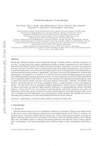
Fig. 1. Negative binomial distribution of the number of noncondensed atoms for an ideal Bose gas in a box with total number of particles N = 10000. it is not the same for the low temperature region T < Tc . Here the broad grandcanonical distribution function does not agree with the well-peacked canonical and micro-canonical distribution function ρ0 (n0 ) around the condensate mean occupation number value. In order to illustrate an actual distribution function, I plot in Fig. 1 the finite negative binomial distribution function of the noncondensate occupation in an ideal Bose gas in the canonical ensemble as is derived within the master-equation approach below in Subsection 4, Eq. (1.53). This is the sharp-peaked statistical distribution which was naively expected for a Bose statistics. The micro-canonical and canonical ensemble formalism do not give the same result in all situations. For different traps the agreement requires additional conditions. For example both ensembles have been found to agree in the large-N (almost thermodynamic limit) case for one-dimensional harmonic trap but to differ in the case of three-dimensional isotropic harmonic trap [21]. In the more general case of d-dimensional σ-power trap, micro-canonical and canonical fluctuations agree in large-N limit when d/σ < 2 and micro-canonical fluctuations become smaller than the canonical ones in the case of d/σ > 2.
19
For large enough particle number N > 105 the calculation of micro-canonical partition function Ω(E, N) becomes very time consuming or even impossible. In this case one can employ the approximation technique based on the saddle-point method which is discussed in details in Chapter V and is widely used in the statistical physics. In this method one starts from the grand-canonical partition function and utilize the saddle-point method for extracting its required canonical and micro-canonical parts. Furthermore, the moments of fluctuations are described by the different order derivatives from the resulting counterparts. Recently, the new type of ensemble was introduce, so called Maxwell’s demon ensemble [20]. In that approach the overall system is divided into two parts: the condensate part and the excited states, which undergo the particle, not energy, exchange between each other. This ensemble gives an approximate result for the ground state fluctuations both in the micro-canonical and canonical ensembles. This approximation can be understood in the framework of the canonical ensemble quasiparticle approach presented in Chapter II. 3. Exact recursion relation for the statistics of the number of condensed atoms in an ideal Bose gas It is worth noting that there is one useful reference result in the theory of BEC fluctuations, namely, an exact recursion relation for the statistics of the number of condensed atoms in an ideal Bose gas. Although it does not give any simple analytical answer or physical insight into the problem, it can be used for “exact” numerical simulations for traps containing a finite number of atoms. It is very useful as a tool to check different approximate analytical solutions. The recursion relation for an ideal Bose gas had been known and used by many authors [20, 21, 23, 27]. In the canonical ensemble, the probability to find n0 particles occupying the single particle
20
ground state is give by: ρ0 (n0 ) =
ZN −n0 (T ) − ZN −no −1 (T ) ; ZN (T )
Z−1 ≡ 1.
(1.38)
The recurrence relation for an ideal Bose gas, thus is: N 1 X ZN (T ) = Z1 (T /k)ZN −k (T ), N k=1
Z1 (T ) = 1 +
∞ X
e−ǫν /T ,
Z0 (T ) = 1,
ν=0
(1.39)
which allows one to numerically evaluate the statistics (1.38). Here ν stands for a set of quantum numbers enumerating a given single particle energy levels ǫν , and the ground-state energy assumed to be ǫ0 = 0 by convention. I will apply the relation (1.39) for evaluation the statistics of an ideal gas in a box in the following sections, in particular, in Chapter II, Section E. An important example is the isotropic, threedimensional harmonic trap, where one has: Z1 (T ) =
∞ X 1 n=0
2
(n + 2)(n + 1)e−n~ω/kB T =
1 (1 − e−~ω/kB T )
3,
(1.40)
where 12 (n + 2)(n + 1) is the degeneracy of the level ǫn = n~ω. There is a similar recurrence relation in the micro-canonical ensemble [20]: N ∞ 1 XX Ω(E, N) = Ω(E − kǫν , N − k), N k=1 ν=0
Ω(0, N) = 1,
Ω(E > 0, 0) = 0, (1.41)
where the sum over ν is finite, since for E < 0 one has Ω(E < 0, N) = 0. Therefore, the ground state occupation probability in the micro-canonical ensemble is: C ρM 0 (n0 ) =
Ω(E, N − n0 ) − Ω(E, N − n0 − 1) ; Ω(E, N)
Ω(E, −1) ≡ 1.
(1.42)
21
4. Dynamical master equation approach Here I outline another approach to the canonical statistics of ideal Bose gases. It was developed in [28] and utilizes a master equation for the condensate in order to find its equilibrium solution. This approach reveals important parallels to the quantum theory of laser and is based on the analogy between a second-order phase transition and laser threshold behavior. The master equation can be simplified in the approximation of detailed balance in the excited states under an assumption that for a given arbitrary number n0 of atoms in the condensate the remaining N − n0 excited atoms are in an equilibrium state at the prescribed temperature T . One can consider the cooling of an ideal noninteracting N-atom Bose gas confined inside a trap. The gas is in contact with a thermal reservoir maintained at the temperature T . The most studies have been concerned with the evaluation of the partition function, which is strongly related to the statistics and thermodynamics of the Bose gas. As it was discussed in [28], one can obtain a simple master equation for the density matrix of the Bose gas as it cools towards the ground state via exchanging the heat with a thermal reservoir. The master equation for the distribution function of the condensed bosons pn0 yields pn˙ 0 = −κ{Kn0 (n0 + 1)pn0 − Kn0 −1 n0 pn0 −1 + Hn0 n0 pn0 − Hn0 +1 (n0 + 1)pn0 +1 }. (1.43) Here κHn0 and κKn0 are the heating and cooling coefficients (which depend upon trap shape, total number of atoms in the trap N and the temperature T ) are similar to the cavity loss and saturated gain parameters in the original laser master equation: Kn 0 =
X
k ′ >0
(ηk′ + 1)hnk′ in0 ,
Hn0 =
X
k ′ >0
ηk′ (hnk′ in0 + 1),
(1.44)
22
where ηk =
1 , exp(ǫk /T ) − 1
X
hnk′ in0 =
nk′
{nk }n0
pn0 ,{nk }n0 . pn 0
(1.45)
One can obtain the steady state distribution of the number of atoms condensed to the ground level of the trap from Eq. (1.43), thus the ground state statistics can be determined. The detailed balance condition involving the cooling and the heating coefficients yields the following expression for the number distribution of the condensed atoms: n0 Y Ki−1
pn 0 = p0
i=1
where the partition function
Hi
,
(1.46)
N N X Y 1 Hi ZN = = pN Ki−1 n =0 i−n +1 0
(1.47)
0
is required to obey the normalization condition
PN
n0 =0
pn0 = 1. The closed form
expression for the coefficients Hn0 and Kn0 can be achieved under different approximations for a different trap shapes. For example, one can apply the so-called “quasithermal” ansatz [28], that stems the same relative average occupation number in the excited levels of the trap as in the thermal reservoir: hnk in0 = ηk
X k>0
hnk in0 /
X k′
ηk′ =
(N − n ¯0) . (exp(ǫk /T ) − 1)H
(1.48)
As the result, one obtains the heating and cooling coefficients as following: Kn0 = (N − n0 )(1 + η),
Hn0 = H + (N − n0 )η,
(1.49)
where H=
X k>0
ηk =
X k>0
1 , exp(ǫk /T ) − 1
η=
X 1 X 2 1 hnk in0 ηk = η . (1.50) (N − n0 ) k H k>0 k
Thus, the analytical formulas for the distribution function of the condensed bosons
23
and the partition function are: � �N −n0 η 1 (N − n0 + H/η − 1)! , pn 0 = ZN (H/η − 1)!(N − n0 )! 1 + η N X N − n0 + H/η − 1 � η �N −n0 ZN = . 1+η N − n0 n0 =0
(1.51)
(1.52)
The explicit formula (1.51) obeys the same canonical recursion relation, which was discussed previously in Section 3. One should emphasize the specific behavior of the ground state occupation probability distribution function. It evolves from a quasithermal peak edged to zero occupation n0 = 0 at T ≈ Tc through a narrow peak centered around some n ¯ 0 6= 0 at T ≈ Tc /2 to a δ-function-like peak near n0 = N for a complete Bose-Einstein condensation at T > (1 + η)H. The master equation (1.43) for pn0 itself, and the analytic approximate expressions (1.51) and (1.52) for the condensate distribution function pn0 and the partition function ZN , respectively, are among the main results of the condensate master equation approach. It provides reasonably accurate description of the first two moments of BEC fluctuations in a Bose gas for a large range of parameters and for different trap potentials. 5. Integral representation via the generalized Zeta function In order to understand relations between various approximate schemes, we formulate a systematic analysis of the equilibrium canonical-ensemble fluctuations of the BEC based on the particle number conserving formalism of Girardeau and Arnowitt [30], the concept of the canonical-ensemble quasiparticles, residue technique and multinomial expansion. This approach will be discussed in details in Chapter II, Section A.
25
In this section I will present an equivalent formulation of the quasiparticle approach in terms of the poles of the generalized Zeta function [31]. Cumulants (semi-invariants) of the BEC fluctuations in an ideal Bose gas can be written in a equivalent form which is quite interesting mathematically [29]. Namely, starting with the cumulant generating function ln Θex (β, z), where β = 1/kB T and z = eβµ , ∞ ∞ X X z n exp[−nβ(ǫν − ǫ0 )] , (1.58) ln Θex (β, z) = − ln(1−z exp[−β(ǫν −ǫ0 )]) = n ν=1 ν=1 n=1 ∞ X
one can use the Mellin-Barnes transform: −a
e
1 = 2πi
Z
τ +i∞
dt a−t Γ(t)
(1.59)
τ −i∞
to write
Z τ +i∞ ∞ X ∞ X 1 zn 1 dtΓ(t) = ln Θex (β, z) = n 2πi τ −i∞ [nβ(ǫν − ǫ0 )]t ν=1 n=1 Z τ +i∞ ∞ ∞ X X 1 1 zn dtΓ(t) = . (1.60) t t+1 2πi τ −i∞ [β(ǫ − ǫ )] n ν 0 ν=1 n=1 P n α Recalling the series representation of the Bose functions gα (z) = ∞ n=1 z /n and
introducing the generalized, “spectral” Zeta function Z(β, t) = [β(ǫν − ǫ0 )]−t , one arrives at the convenient (and exact) integral representation: 1 ln Θex (β, z) = 2πi
Z
τ +i∞
dtΓ(t)Z(β, t)gt+1(z).
(1.61)
τ −i∞
d gα (z) = gα−1 (z) and Applying the well-known relation for the Bose functions z dz
gα (1) = ζ(α), where ζ(α) denotes the original Riemann Zeta function, Eq. (1.61) can be rewritten in terms of the cumulants of the distribution function as: � �k Z τ +i∞ ∂ 1 κk (β) = z dtΓ(t)Z(β, t)ζ(t + 1 − k). ln Θex (β, z)|z=1 = ∂z 2πi τ −i∞
(1.62)
Thus, by means of the residue theorem, Eq.(1.62) links all cumulants of the canonical
26
distribution function in the condensate regime to the poles of the generalized Zeta function Z(β, t), which contains all the system properties, and to the pole of a systemindependent Riemann Zeta function, the location of which depends on the order k of the respective cumulant. The formula (1.62) provides a systematic asymptotic expansion of the cumulants κk (β) through the residues of the analytically continued integrands, taken from right to left. The large system behavior extracted from the condensate fluctuations is definitely seen. The details and examples of such analysis can be found in [31]. I would like to emphasize that none of the presented above theories can describe the mesoscopic behavior of the confined Bose gas in the trap without using some approximations, and there is no yet a complete and general theory of the BEC fluctuations.
C. Mesoscopic systems Successful experimental demonstration and various recent experiments on the BoseEinstein condensation (BEC) in the magneto-optical traps strongly demand a development of a theory of the BEC phase transition in the actual mesoscopic systems containing a finite number of atoms N ∼ 102 − 106 in a finite-size trap (for a review, see e.g. [20] and references therein). One of the most important problems is to find the universal, common to the mesoscopic systems of any size, features in the behaviour of an order parameter, i.e., a mean number of atoms in the condensate n ¯ 0 , and its fluctuations as the functions of the number of atoms in the trap and the temperature T in the critical region, T ∼ Tc or N ∼ Nc , as well as above and below it. In the statistical physics until recently most studies were done for the macroscopic systems in the thermodynamic, or bulk, limit when both a volume V and a number
27
of atoms N in the trap tend to infinity [5, 22, 32–34]. An opposite limit of a very few atoms in the trap (N = 1, 2, 3, ) corresponds to a microscopic system studied by the methods of a standard quantum mechanics. An intermediate case of a mesoscopic number of atoms is the most difficult for it requires a solution that explicitly depends on the number of atoms in the trap. Besides, for the mesoscopic systems an inapplicability of the standard in the statistical physics approaches, for example, a grand-canonical-ensemble method and a BeliaevPopov diagram technique [5, 8, 22, 34], becomes especially obvious, in particular, for the analysis of the anomalous fluctuations in the critical region. A simple example is given by a well-known grand-canonical catastrophe of the BEC fluctuations [20, 33, 34]. To get the solution of the BEC phase transition problem right, the most crucial P issue is an exact account for a particle-number constraint n ˆ 0 + k6=0 n ˆ k = N = const
as an operator equation which is responsible for the very BEC phenomenon and is equivalent to an infinite set of the c-number constraints. It cannot be replaced by just one condition for the mean values, N = n ¯0 + n ¯ , used in the grand-canonical-ensemble approach to specify an extra parameter, namely, a chemical potential µ. Here n ˆ k is P an occupation operator for a k-state of an atom in the trap and n ˆ = k6=0 n ˆ k is a total occupation of the excited states.
Thus, we have to find an explicit solution to a statistical problem of BEC for a finite number of atoms in the trap in a canonical ensemble. Some results in this direction are known in the literature, however, a clear and full physical picture of the statistics and dynamics of BEC in the mesoscopic systems is absent until now not only in a general case of an interacting gas, but even in the case of an ideal gas (for a review, see e.g. [20, 34] and references therein). In particular, one of the most interesting in the statistical physics of BEC results, namely, a formula for the anomalously large variance of the ground-state occupation, h(ˆ n0 − n ¯ 0 )2 i ∝ N 4/3 (T /Tc )2 , found both
28
for the ideal gas [34] and for the weakly interacting gas [21, 35, 36], is valid only far enough from the critical point, when fluctuations of the order parameter are already relatively small, h(ˆ n0 − n ¯ 0 )2 i1/2 N, in all operator equations and under all trace operations. That θ(N − n ˆ ) factor is the constraint nonlinearity
that, being accepted, allows one to consider the noncondensate many-body Fock space formally as an unconstrained one. Therefore properly normalized constrained distribution function exactly obeys the well-known recursion relation for an ideal gas and N-particle constraint, by its construction, which makes it truly a solution of the problem. In Section D of the Chapter II I describe in some details the spectrum of a box trap that is used as a particular example for the numerical simulations in the dissertation. For the analysis of non-Gaussian properties it is convenient to consider cumulants (semi-invariants) κm which are related to the central moments µm = h(n − n ¯ )m i and “generating cumulants” κ ˜m by the following relations: κ1 = n ¯,
κ2 = µ2 ,
κ5 = µ5 − 10µ2 µ3 ,
κ3 = µ3 ,
κ4 = µ4 − 3µ2 2 ,
� κ6 = µ6 − 15µ2 µ4 − 2µ22 ,
(1.63)
30
κ1 = κ ˜1 , κ3 = κ ˜ 3 + 3˜ κ2 + κ ˜1 ,
κ2 = κ ˜2 + κ ˜1, κ4 = κ ˜ 4 + 6˜ κ3 + 7˜ κ2 + κ ˜ 1 , ...
(1.64)
In Section E of the Chapter II I present the closed-form, analytical expression for the distribution function and its cumulants and obtain the expansion in terms of the multinomial coefficients. In Section F I compare the condensate statistics for the finite system with its thermodynamic limit and present the expressions for the low and high temperature asymptotics for the first few cumulants of ground state statistics for both ideal and weakly interacting Bose gas. In Chapter III I introduce a universal constraint nonlinearity responsible for the phase transition through a reduction of the many-body Hilbert space. I calculate a probability distribution of the number of atoms in the condensate n0 that is complimentary to the total number of atoms in the excited states (noncondensate) n = N − n0 and explain a remarkable constraint-cut-off mechanism that makes BEC fluctuations strongly non-Gaussian in the critical region (Section A). On this basis I find the universal scaling and structure of the BEC statistical distribution (Section A) as well as of the order parameter (Section B) and all higher-order moments and cumulants (Section C) of the BEC statistics for any number of atoms trapped in a box with any volume V = L3 and temperature. I prove that these results perfectly match the known values of the statistical moments in the low-temperature region (T > Tc ), where there is no condensate [32–34]. Finally, I demonstrate that the described constraint-cut-off mechanism does yield the strongly non-Gaussian BEC fluctuations, similar to the ones found for the ideal gas in the box, even if one employs a pure Gaussian model for an unconstrained probability distribution of the noncondensate occupation that corresponds to an exactly solvable
31
model of BEC in a degenerate interacting gas (Section D). In Chapter IV I describe a two-level trap model for the BEC of the ideal gas and its exact solution for the constrained distribution function and its cumulants in the form of the cut-off negative binomial distribution (Section A) and its continuous approximation - cut-off gamma distribution (Section B). In Section C, I compare the results of both models as well as a 3-level trap model against BEC statistics in a real box trap and find an extent of validity of the so-called quasithermal ansatz [21]. The parameters for the 3-level trap are offered in the sense to fix the behavior of the first few cumulants. In the case when the second level coincides with the first excited state of the trap one can observe the perfect agreement between first two and all high order cumulants calculated in the 3-level model with the exact solution for the BEC in the box. In Chapter V I employ the refined saddle-point approximation to obtain the asymptotic expression for the distribution function of condensed atoms in an ideal gas in a trap. In Section A, following [27], I formulate the method for the case of a harmonic trap and explain why the standard saddle-point approximation does not work for the systems with condensate. Then in Section B I employ this method to find the condensate distribution function in an ideal gas in a box. In Section C I do numerical simulations and compare the asymptotical results obtained by the refined saddle-point approximation and constraint nonlinearity method in Chapter III for the distribution function. Finally, I shortly discuss still open problem of an applicability of the saddle-point approximation in the BEC statistics. In Chapter VI I summarize the main results on BEC statistics presented in the dissertation. In Appendices A, B, C I present the detailed derivation of the characteristic function and the initial statistical moments of the ground state occupation as well as
32
the residue technique and derivation of the multinomial expansion for the condensate statistics.
33
CHAPTER II
QUANTUM STATISTICS OF THE IDEAL AND WEAKLY INTERACTING BOSE GASES IN A BOX IN THE CANONICAL ENSEMBLE. A. Canonical ensemble quasiparticle approach The standard methods of thermodynamics are not appropriate for the analysis of BEC fluctuations and mesoscopic effects. For example, the most widely known grandcanonical approach suffers from the grand-canonical catastrophe [38]. The restricted ensemble approach, which fixes the amplitude and the phase of the condensate wave function, is unable to analyze the fluctuation problem at all. To study the fluctuations, one should fix only external macroscopical and global, topological parameters of the system such as temperature, pressure, number of particles, super-fluid flow pattern, boundary conditions, etc. Solving the Von Neuman equation with general initial conditions one can get all possible states of the condensate. For the real systems, even with a weak interaction this way is very complicated. The perturbative series involving the initially unperturbed grand-canonical ensemble do not converge [8], thus it is impossible to use them. One way to handle this problem is to deal with constrained many-body Hilbert space. The possibility of the proper reduction of the Fock space arises from introducing the new canonical ensemble quasiparticles. The usual particle number representation in many-body Hilbert space can be written as a proper combination of creation and annihilation operators a ˆ†k and a ˆk , which act as following (n)
aˆ†k |ψk i =
√
(n)
n + 1|ψk i,
(n)
a ˆk |ψk i =
√
(n−1)
n|ψk
i,
(n)
(n)
n ˆ k |ψk i = n|ψk i.
(2.1)
Girardeau and Arnowitt (GA) [30, 37] were the first who introduced the creation and
34
annihilation operators acting in the canonical ensemble subspace of the Fock space which takes into account the particle number constraint. These operators obey the usual Bose commutation relations for k 6= 0 in the subspace with n0 6= 0, namely,
βˆk† = a ˆ†k βˆ0 ,
ˆk , βˆk = βˆ0† a
βˆ0 = (1 + n ˆ 0 )−1/2 a ˆ0 ,
h i † ˆ ˆ βk , βk′ = δk,k′ .
(2.2)
Since the GA operator subspace excludes states with zero number of the condensed atoms, this approach will be relevant for almost all temperatures T < Tc , starting even from a small condensate fraction n ¯ 0 1. The standard Bogoliubov transformation βˆk = ukˆbk + vkˆb†−k ; βˆk† = ukˆb†k + vkˆb−k ;
1 Ak , vk = p , 2 1 − Ak 1 − A2k � � ~2 k2 n ¯ 0 Uk V ǫk − , − Ak = n ¯ 0 Uk 2m V uk = p
(2.8)
determines dressed by condensate canonical-ensemble quasiparticles that fluctuate independently according to approximation in Eq. (2.6). One can rewrite the atomnumber-concerving Hamiltonian from Eq. (2.6) in terms of new dressed quasiparticles
36
in Eq. (2.8) as follows: HB = E0 +
X
ǫ˜kˆb†kˆbk ,
(2.9)
k6=0
where a “gapless” Bogoloubov energy spectrum is s� �2 � �2 ¯ 0 Uk n ¯ 0 Uk ~2 k2 n ǫ˜k = + − . 2m V V
(2.10)
It is now clearly seen that we arrive to the problem of an ideal gas of dressed quasiparticles in contrast to the gas of atoms and gas of bare quasiparticles in Eq. (2.2). Therefore, the analysis of fluctuations can be performed simultaneously in the same fashion in both cases of ideal gas and weakly interacting gas.
B. Characteristic function for the ground state occupation number in an ideal Bose gas From the construction of the canonical-ensemble quasiparticles outlined in the previous section (see Eq. (2.2)), one concludes, that the occupation numbers nk can be approximated as an independent stochastic variables and, thus, one can apply an equilibrium distribution to the equilibrium canonical ensemble density matrix: ρk (nk ) = exp (−nk ǫk /T ) [1 − exp (−ǫk /T )] .
(2.11)
The distribution function of the excited atoms according to Eq. (2.4) is just a mirror distribution of the condensed particles: ρ (n) = ρ0 (n0 = N − n) .
(2.12)
37
In statistical physics there is a useful formalism of describing the density matrix via the characteristic function: Θn (u) = Tr{eiun ρˆ},
Θn (u = 0) = 1.
(2.13)
Taking the inverse Fourier transformation, one obtains the distribution function 1 ρ (n) = 2π
Z
π
e−inu Θn (u) du.
(2.14)
−π
Very important property of the characteristic function is that the characteristic function for the ensemble of the independent stochastic variables is a product of the individual characteristic functions, thus: Θn (u) =
Y
Θnk (u) ,
ln Θn (u) =
k6=0
X
ln Θnk (u) .
(2.15)
k6=0
Each individual characteristic function can be easily calculated from the equilibrium density matrix as following: � zk − 1 Θnk (u) = Tr{eiuˆnk ρˆk } = Tr{eiuˆnk e−ǫk nˆ k /T } 1 − e−ǫk /T = , zk − z
(2.16)
where zk = exp (ǫk /T ) and z = exp(iu) is a fugacity. Therefore, for an ideal gas in an arbitrary trap, the characteristic function of the number of excited atoms can be written as Θn (u) =
Y zk − 1 . iu z k −e k6=0
(2.17)
In the case of weakly interacting dilute gas the equilibrium density matrix is not diagonal in the basis of bare atoms, which statistics we want to calculate. It can be written as follows: ρˆ =
Y
k6=0
ρˆk ,
ˆ† ˆ
ρˆk = e−ǫk bk bk /T (1 − e−ǫk /T ).
(2.18)
38
The mentioned above effect leads to the squeezing of fluctuations effect which is wellknown in laser physics. The number of atoms with coupled momenta k and −k can be written in terms of Bogoliubov coupling coefficients as follows: † ˆ a ˆ†k aˆk = βˆk† βˆk + βˆ−k β−k =
= (u2k + vk2 )(ˆb†kˆbk + ˆb†−kˆb−k ) + 2uk vk (ˆb†kˆb†−k + ˆbkˆb−k ) + 2vk2 .
(2.19)
The characteristic function for the total number of atoms in the two k and −k modes squeezed by Bogoliubov coupling was calculated in [21] as follows: h i ˆ† ˆ ˆ† ˆ ˆ† ˆ ˆ† ˆ Θ±k (u) = Tr eiu(βk βk +β−k β−k ) e−ǫk (bk bk +b−k b−k )/T (1 − e−ǫk /T )2 = =
[z(Ak ) − 1][z(−Ak ) − 1] , [z(Ak ) − eiu ][z(−Ak ) − eiu ]
(2.20)
where z(Ak ) =
Ak − eǫk /T . Ak eǫk /T − 1
(2.21)
The characteristic function for the total number of the excited atoms is equal to the product of the couple-mode characteristic functions, Θn (u) =
Y
Θ±k (u),
(2.22)
k6=0,mod(±k)
where the product runs over all different pairs of (k, −k), since these modes are independent to the first approximation (see Eq. (2.6)). The characteristic function or its logarithm can be expanded as a Taylor series with cumulants (semi-invariants), generating cumulants or initial (noncentered) moments as the coefficients [29]: Θn (u) =
∞ X
m=0
αm
(iu)m , m!
αm ≡ hnm i =
dm Θn (u)|u=0, d(iu)m
(2.23)
39
∞ X
(iu)m dm , κm = ln Θn (u)|u=0, m! d(iu)m m=1 ∞ ∞ m X � zk − 1 � X X (iu)m (eiu − 1) ln = κm ln Θn (u) = = κ ˜m . z m! m! k−z m=1 m=1 k6=0 ln Θn (u) =
κm
(2.24)
(2.25)
The cumulants κm and generating cumulants κ ˜ m can be related by the Stirling numbers of the second kind [29]:
σr(m) =
1 m!
m X
m r (−1)m−k k , k k=0
(ex − 1)k = k!
∞ X
σn(k)
n=k
xn . n!
(2.26)
The useful property is that the cumulant of the sum of independent stochastic variP ables is equal to a sum of the partial cumulants κr = k6=0 κkr . This relation follows from the productivity property of the characteristic function (2.15). Also the cumu-
lants can be simply related to the initial (noncentered) and central moments of the distribution by binomial relations [29]: r X r ¯k , µr = (−1)k αr−k n k k=0 n ¯ = κ1 ,
�
(n − n ¯ )2 ≡ µ2 = κ2 ,
αr =
r X r ¯k µr−k n k k=0
(2.27)
�
(n − n ¯ )3 ≡ µ3 = κ3 ,
�
(n − n ¯ )4 ≡ µ4 = κ4 + 3κ2 2 ,
� (n − n ¯ )5 ≡ µ5 = κ5 + 10κ2 κ3 ,
� � (n − n ¯ )6 ≡ µ6 = κ6 + 15κ2 κ4 + 2κ22 ,
(2.28)
κ4 = κ ˜ 4 + 6˜ κ3 + 7˜ κ2 + κ ˜ 1 , ....
(2.29)
κ1 = κ ˜1,
κ2 = κ ˜2 + κ ˜1,
κ3 = κ ˜ 3 + 3˜ κ2 + κ ˜1 ,
In the case of low temperatures, far enough from the region near the critical temperature of the Bose condensate, where the properties of the moments except for the
40
average value do not depend on the total number of atoms in a trap, i.e. the mesoscopic effects are not important, the cumulants of the condensate distribution can be written as: X (eǫk /T − 1)−m ; κ ˜ m = (m − 1)! k6=0
κr =
∞ X
σn(k) κ˜m .
(2.30)
n=k
Similar to Eq. (2.30), in the case of weakly interacting gas, all cumulants can be written as follows � X� 1 1 1 κ ˜ m = (m − 1)! + . 2 [z(Ak ) − 1]m [z(−Ak ) − 1]m
(2.31)
k6=0
In comparison with the ideal Bose gas in Eq. (2.30), we have a mixture of two species of atom pairs with z(±Ak ) instead of exp(ǫk /T ). It is worth noting that Eq. (2.31) for m = 1 is a non-linear self-consistency equation, N −n ¯ 0 = κ1 (¯ n0 ) ≡
X k6=0
1 + A2k eǫk /T , (1 − A2k )(eǫk /T − 1)
(2.32)
for the mean ground state occupation number n ¯ 0 (T ), since the Bogoluibov coupling coefficient Ak in Eq. (2.8) and energy spectrum ǫk in Eq. (2.10) are the functions of n ¯ 0 . Therefore, the rest of the Eqs. (2.31) for m ≥ 2, are nothing else but explicit expressions for all cumulants, m ≥ 2, if one substitutes the solution of the selfconsistency Eq. (2.32) for the mean value n ¯ 0. These formulas are valid in the case of condensate inside the infinite reservoir of the excited atoms. This universal result was found in [21] and is equivalent to the Maxwell’s demon ensemble approximation. In particular, this result does not describe many mesoscopic effects and the temperature range near and above critical temperature Tc .
41
C. Constraint nonlinearity and many-body Fock space cut-off in the canonical ensemble As it was discussed in previous sections and in [39–42], the only reason for the BEC of atoms on the ground state k = 0 is the conservation of the total number of the Bose particles in the trap, N = n ˆ0 + n ˆ . Hence, the occupation operators n ˆ k are not independent and the many-body Hilbert space is strongly constrained. A more convenient equivalent formulation of the problem can be given if one introduces a constraint nonlinearity in the dynamics and statistics, even for the ideal gas, on the basis of the particle-number constraint. In most previous studies, an actual (e.g., micro-canonical or canonical) quantum ensemble was substituted by an artificial grand-canonical ensemble, where only the mean number of particles is fixed by the appropriate choice of the chemical potential µ and, therefore, most quantum effects in dynamics and statistics of BEC were lost or misunderstood. Following our general approach [20, 21, 35, 39–42], we solve for the constraint from the very beginning through the proper reduction of the many-body Hilbert space. In the present case of the ideal gas in the canonical ensemble, we have to consider as independent only noncondensate Fock states {nk , k 6= 0}i which uniquely specify the P ground-state Fock state n0 = N − k6=0 nk i. However, the remaining noncondensate Fock space should be further cut off by the boundary nk ≤ N. The latter is equivalent
to an introduction of a step-function θ(N − n ˆ ), i.e., 1 if n ≤ N or 0 if n > N, in all operator equations and under all trace operations. That θ(N − n ˆ ) factor is the constraint nonlinearity that, being accepted, allows us to consider the noncondensate many-body Fock space formally as an unconstrained one. We adopt this point of view from now on. Therefore, the BEC fluctuations are described by a mirror image of the proba-
42
bility distribution of the total number of excited (noncondensed) atoms ρn = ρcond (n0 = N − n),
1 ρn = 2π
Z
where iun
Θn (u) = Tr{e
ρˆ θ(N − n ˆ )} =
π
e−iun Θn (u)du,
(2.33)
−π
N X
eiun ρn
(2.34)
n=0
is a characteristic function for the stochastic variable n, ρˆ = e−H/T /Tr{e−H/T θ(N −n)} is an equilibrium density matrix, and the temperature is measured in the energy units, so that the Boltzmann constant is set to be 1. Thus, the actual probability distribution ρn =
ρn(∞) /
N X
ρn(∞)
(2.35)
n=0
(∞)
is merely a θ(N − n) cut off of the unconstrained probability distribution ρn
for an
infinite interval of the noncondensate occupations n ∈ [0, ∞), as is shown in Fig. 2. (∞)
The latter distribution ρn
was analytically calculated in [21, 35] (see Section B
of this chapter) via all its moments and cumulants for arbitrary trap. Thus, only a straightforward calculation of the moments and cumulants of the cut off probability distribution, given in Eq. (2.35) and depicted as a curve OAN in Fig. 2, remains to fulfill in order to find the actual BEC statistics in the mesoscopic system for all numbers of atoms and temperatures, including a critical region.
D. Properties of the spectrum of the box with the periodic boundary conditions In this section I explain the subtle points of the momentum summation (product) that occurs in the different statistical quantities in Bose gas in a box with periodic boundary conditions. I will make the analysis for the case of the ideal gas energy spectrum for the simplicity, because it is not essentially a property of the gas or interaction but is the property of the periodic boundary conditions for cartesian
43
Ρn 0.033
A
ΡnH¥LHxL
A'
0
n' N'
n Nc N
n 100
Fig. 2. Unconstrained probability distribution of the number of noncondensed atoms (∞) ρn (dashed line) and its cuts off (solid lines) for a small number of atoms N ′ < Nc (OA′N ′ , there is no condensate) and for a large number of atoms N > Nc (OAN, there is condensate) for the trap with a given volume and temperature: the trap-size parameter in Eq. (3.2) is Nv = 100.
44
planar boundaries following from the Fourier analysis in the basis of the simplest trigonometric functions. Consider an atomic gas with a mass m in the 3D box of a volume L3 with periodic boundary conditions, which looks almost like a free particle spectrum, beside the certain quantized momentum ~kl , ǫk =
~2 k2 , 2m
kl =
2π l, L
The characteristic quantity zk = eǫk /T = eǫ1 l
2 /T
l = (lx , ly , lz ).
(2.36)
has the meaning of the inverse prob-
ability of finding particle in the state with energy ǫk , and the energy gap parameter is ǫ1 /T = (2π~/L)2/(2mT ).
(2.37)
It is obvious, that the critical temperature is different for different number of particles, even though the temperature scale is always the critical temperature for the thermodynamic limit of an ideal gas in a box: 2π~2 Tc = m
�
N 3 L ζ(3/2)
�2/3
,
(2.38)
so that � � n ¯0 = N − n ¯ = N − κ1 = N 1 − (T /Tc )3/2 .
(2.39)
One can simplify the summation involved in the computation of cumulants and product in characteristic function by applying the symmetry of the boundaries and spectrum. Let us focus on the summation, for instance. One has the sum over all modes beside the mode with zero energy - the excluded zero origin. This summation can be performed over different 3D, 2D, and 1D submanifolds in the momentum space of the box separately. It is obvious that modes with k and −k have the same energy. For 3D subspace one has 8 equivalent domains with positive (kx , ky , kz ) and 6 ways of rearranging them in the order, for example: kx > ky > kz or kx > ky < kz , etc. The total
45
degeneracy will be 8 · 6 = 48. Similarly, one can obtain the following degeneracies for 2D submanifold: 4 · 3 = 12 domains for the pair and 2 ways of rearranging kx < ky or kx > ky , thus the total 2D degeneracy is 24. Note, that 1D submanifold contains three types of subvolumes; namely a domain where for example: kx 6= 0, ky = kz = 0 with degeneracy 2 · 3 = 6, corresponding to the ribs of the cube, kx = ky 6= 0, kz = 0 with degeneracy 4 · 3 = 12, corresponding to the diagonals of each of eight sides of the cube and domain with kx = ky = kz 6= 0 with degeneracy 8, as a diagonal in each of eight quadrants of positive or negative k-axis. Thus, one can conclude, that the summation (product) of an arbitrary function f (k) over all momentum space with excluded origin can be written as: X
f (k) =
k6=0
X
X
f (kx , ky , kz ) +
kx ≥ky >kz >0
k≡(kx ,ky ,kz )6=0
24
X
f (kx , ky , kz ) = 48
f (kx , ky , 0) + 6
kx >ky >0
X
f (kx , 0, 0) + 12
kx >0
+8
X
X
f (kx , kx , 0)+
(2.40)
kx >0
f (kx , kx , kx ).
kx >0
For example, the characteristic function (2.17) of the total number of noncondensed particles can be written as: !48 2 2 2 ∞ ∞ ∞ Y zk − 1 Y Y Y eǫ1 (kx +ky +kz )/T − 1 × Θ(z) = = zk − z k =1 k =k +1 k =k eǫ1 (kx2 +ky2 +kz2 )/T − z k6=0 z y z x y !24 ∞ !6 2 2 ∞ ∞ Y eǫ1 (kx2 )/T − 1 Y Y eǫ1 (kx +ky )/T − 1 × × 2 2 eǫ1 (kx2 )/T − z eǫ1 (kx +ky )/T − z kx =1 ky =1 kx =ky +1 !12 ∞ !8 2 ∞ Y eǫ1 (3kx2 )/T − 1 Y eǫ1 (2kx )/T − 1 . × eǫ1 (2kx2 )/T − z eǫ1 (3kx2 )/T − z k =1 k =1 x
(2.41)
x
The difference in summation rule for the case of weakly interacting gas is that the summation is performed on pairs of (k, −k) which makes the degeneracies to be one P P half of corresponding degeneracies in the ideal gas: 2 k6=0,mod(k,−k) = k6=0 .
46
E. Multinomial expansion The following discussion will be dedicated to the derivation of the closed form expression for the distribution function, its cumulants, as well as the initial and central moments for the ideal and weakly interacting dilute Bose gases using the combinatorial analysis of the multinonial coefficients. The detailed derivation of the following formalism is presented in Appendices A-C. Let us start with a simpler case of an ideal gas. Consider the characteristic function of the total number of noncondensed atoms given in Eqs. (2.15)-(2.17). It can be written as following: Θ (z) =
Y zk − 1
k6=0
zk − z
where z = eiu , Θ0 ≡ Θ(z = 0) =
= Θ0 exp − Q
k6=0
zk −1 zk
X k6=0
!
ln(1 − z/zk ) ,
(2.42)
is the characteristic function at zero
fugacity z. Employing the Taylor expansion of the logarithm under the summation about the point z = 0 and changing the summation order in the exponent power, one can rewrite (2.42) as following Θ(z) = Θ0 exp
∞ X
fm z m
m=1
!
,
(2.43)
where coefficients in Taylor expansion above are fm ≡ fm (z = 0), fm (z) = zk )−m .
P
k6=0 (z
−
Employing the approach discussed in the Appendix A of expressing the condensate statistics as a residues of the characteristic function evaluated at z = 0 (see Eq. (A.4)) one can conclude, that ρ(n) is nothing else but the Taylor coefficient of the z n term, Θ0 d n ρ(n) = n! dz n
∞ X 1 r! r=0
∞ X
m=1
fm z
m
!r !
z=0
,
(2.44)
since all the other are zero. Here and in Appendices by ρ(n) I mean an unconstrained
47
(∞)
distribution function ρn . One can now employ the wonderful properties of the multinomial coefficients [29]: !r ∞ ∞ X X zn X m fm z ≡ r! (n; a1 , a2 , a3 ..., an )∗ f1a1 f2a2 f3a3 ...fnan , n! m=1 n=r
(2.45)
summed over a1 + a2 + a3 + ... + an = r and a1 + 2a2 + 3a3 + .. + nan = n, where the multinomial coefficients have the following closed form expression: (n; a1 , a2 , a3 ..., an )∗ = n!/1a1 a1 !2a2 a2 !3a3 a3 !...nan n!,
(2.46)
with the same restricted summation a1 + 2a2 + 3a3 + .. + nan = n. The meaning of these coefficients is the number of permutations of n = a1 + 2a2 + 3a3 + .. + nan symbols composed of ak cycles of length k for k = 1, 2, 3, ..., n. Applying the expression (2.45) to obtain the distribution function and changing the summation order as well as employing the fact, that n-th derivative is non zero only for n-th term in the expansion, the result can be written as: n Θ0 X ρ(n) = n! m=0 0 B B B B @
X
(n, a1 , a2 , ..., an )
a1 + a2 + ... + an = m a1 + 2a2 + ... + nan = n
1 C C C C A
∗
n Y
a
fj j .
(2.47)
j=1
This closed form expression for the distribution function is exact and no approximations were implied so far. The initial moments of the distribution function presented in Eq. (2.47) which can be calculated also via the Taylor expansion of the constrained characteristic P m function, Θn (u) = N m=0 αm u /m! are related to the central moments µm = h(n − n ¯ )m i and to the cumulants κm by the following explicit formulas [29]: αr =
r X k=0
Crk µr−k n ¯k ,
µr =
r X k=0
(−1)k Crk αr−k n ¯k ,
(2.48)
48
κr =
r X
m=1
(−1)m − 1(m − 1)!
αm =
m X X
X
(r; a1 , ..., ar )′ α1a1 ...αrar ,
(2.49)
(r,m)
(m; a1 , ..., am )′ κa11 ...κamm ,
(2.50)
r=1 (m,r)
where Crk = r!/(k!(r − k)!), (m; a1 , ..., am )′ = m!/((1!)a1 a1 !(2!)a2 a2 !...(m!)am am !) is a multinomial coefficient, and the sum in Eqs. (2.49)-(2.50) runs over the nonnegative integers a1 , ..., ar which satisfy the following two conditions: a1 + 2a2 + ... + rar = r and a1 + a2 + ... + ar = m. We calculate the quantities which are the most important and convenient for the analysis of the BEC statistics, namely, the mean value n ¯ (which is complimentary for the BEC order parameter n ¯0 = N − n ¯ ) as well as the central moments µm and cumulants κm of the total noncondensate occupation. The point is that the ground-state (condensate) occupation fluctuates complimentary to a sum of many, to a large extent independent occupations of the excited states in the noncondensate, conditioned by the particle-number constraint. The central moments of the condensate fluctuations differ from the corresponding central moments of the noncondensate fluctuations only by the sign for the odd orders, h(n0 − n ¯ 0 )m i = (−1)m h(n − n ¯ )m i. The centered moments calculated with such a distribution function coincide perfectly with the exact recursion relation of Eq. (1.38): ρ0 (n0 ) =
ZN −n0 (T ) − ZN −no −1 (T ) ; ZN (T )
Z−1 ≡ 1,
N 1 X Z1 (T /k)ZN −k (T ), ZN (T ) = N k=1 X Z1 (T ) = 1 + e−ǫk /T .
(2.51)
(2.52)
k6=0
Similar analysis can be performed in the case of weakly interacting gas. Starting from the characteristic function of the total number of noncondensed atoms given in
49
Eq. (2.20) one can express it in the following form: Y
Θn (z) =
=
k6=0,mod(±k)
[z(Ak ) − 1][z(−Ak ) − 1] = [z(Ak ) − z][z(−Ak ) − z]
! 1X 1X ln[1 − z/z(Ak )] − ln[1 − z/z(−Ak )] , = Θ0 exp − 2 k6=0 2 k6=0 where Θ0 ≡ Θ(z = 0) =
Q
k6=0,mod(±k)
=
[z(Ak )−1][z(−Ak )−1] z(Ak )z(−Ak )
(2.53)
is a characteristic function
at zero fugacity z. It is obvious that one has two similar contributions from both z(±Ak ) in the exponent compare to the case of the ideal gas, where one has one term with zk . The factor 1/2 in front of these two terms is following from the summation P P rule discussed in the previous section, in particular: k6=0,mod(k,−k) Θk = 12 k6=0 Θk . Performing calculation similar to the case of the ideal gas one arrives to essentially
the same Eq. (2.47) but with different coefficients fm . In the case of weakly interacting gas these coefficients also have two additive terms: fm ≡ fm (z = 0), P fm (z) = 21 k6=0 [(z − z(Ak ))−m + (z − z(−Ak ))−m ]. The existence of two additive
contributions to the different quantities in the presence of interaction modifies also a single particle partition function. In contrast with the ideal gas one need to rewrite Eq. (2.52) as follows: Z1 (T ) = 1 +
� 1X z(Ak )−1 + z(−Ak )−1 . 2 k6=0
(2.54)
Beside the presented above modification of single-particle partition function, the recursion relation in Eq. (2.51) remains unchanged. Therefore, one can compare the condensate statistics obtained from the multinomial expansion and by means of recursion relation in both cases of the ideal and weakly interacting gas. The perfect match can be observed by numerical simulations. The resulting temperature scaled first four central moments of the ground state occupation fluctuations for an ideal
50
gas in a box, calculated from the Eqs. (2.50) and (2.48) for N = 100 using the multinomial expansion formalism in Eq. (2.47) and exact recursion relation for both cases of the ideal and weakly interacting gas in Eq. (2.51) are presented in figures on pages 55-58.
F. Mesoscopic effects versus the thermodynamic limit In this section, I summarize the results obtained in the previous section for the mesoscopic condensate statistics and compare it to the thermodynamic limit statistics, obtained in [21] for both ideal and weakly interacting Bose gas in a box. The first four central moments of the distribution function in the mesoscopic system can be found by plugging in the distribution function (2.47) into the expressions for the initial moments (2.50) and for the central moments (2.48). The expressions for the first four central moments in the thermodynamic limit are obtained through the cumulants (2.30) for the case of ideal gas and (2.31) in the case of weakly interacting gas, generating cumulants (2.29), and their connection to the central moments (2.28). For the particular case of an ideal Bose gas in a box it can be written as follows: κ ˜ m = (m − 1)!
X
ǫ1 l2 /T
(e
l={lx ,ly ,lz }6=0
−m
− 1)
;
κr =
∞ X
σn(k) κ ˜m ,
(2.55)
n=k
where the energy gap parameter ǫ1 is defined in Eq. (2.37). n ¯ = κ1 ,
� (n − n ¯ )2 ≡ µ2 = κ2 ,
� (n − n ¯ )3 ≡ µ3 = κ3 ,
� (n − n ¯ )4 ≡ µ4 = κ4 + 3κ2 2 .
(2.56)
51
If the temperature is much smaller than the energy gap T Tc the condensate fraction is small n ¯ 0 ǫ1 =
�
2π~ L
�2
1 , 2m
(2.67)
so that the border T ǫ˜1 between the moderate temperature and very low temperature regimes is shifted to higher temperatures. Another important effect of the weak interaction is a suppression of all condensate-fluctuation cumulants by a factor of 1/2, compared with the ideal gas (see Eq. (2.31)), for the moderate temperatures ǫ˜1 2 (ζ(3/2))2/3N 1/3 n ¯0, Tc L
(2.78)
where I explicitly used the expression for the interaction strength in term of the swave scattering length, U0 = 4π~2 a/m. Depending on the interaction strength one can analyze the asymptotical behavior of the fluctuations at temperatures of the order of Tc . This condition is satisfied for a wide range of parameters in real experiments [12–14] and thus can be used to illuminate the crossover between the fluctuations in the ideal and weakly interacting Bose gases. I would like to emphasize that the above crossover relations, i.e. the high temperature asymptotics, were derived using
61
the particle-number constraint, the canonical ensemble quasiparticle formalism, and the multinomial expansion. Concluding the whole chapter, I briefly emphasize its main points. First, I constructed the set of canonical ensemble quasiparticles (GA operators) which take into account the particle number constraint. Using the outlined method I analyzed the structure of the characteristic function of the total number of noncondensed atoms in both ideal and weakly interacting Bose gas. The latter case was analyzed in the framework of Bogoliubov dressed quasiparticles. Then I introduced the new properly normalized distribution function, which correctly describes the behavior of the ground-state fluctuations in any temperature regime, which was constructed from the simple physical reasons. I obtained the numerical dependences for the fluctuations for the mesoscopic system of an ideal and weakly interacting Bose gas in a box with periodic boundary conditions as the functions of temperature. All the listed calculations are valid for the whole temperature range from zero to infinity. I considered the asymptotic expressions for the fluctuations for both low and high temperatures and compared them with the well know grand canonical formalism for high temperatures, where both ideal and weakly interacting gas give the same answer. For the low temperature the dressed condensate fluctuations for the interacting gas are depleted compare the bare fluctuations in the ideal gas. For the moderate temperatures I found a crossover relations between fluctuations of weakly interacting gas and ideal gas. In the next chapter I will discuss another approach in analyzing these fluctuations, in the vicinity of the critical temperature.
62
CHAPTER III
UNIVERSAL SCALING AND ORIGIN OF NON-GAUSSIAN BOSE-EINSTEIN CONDENSATE STATISTICS IN A MESOSCOPIC IDEAL GAS A. Constraint-cut-off mechanism of strong non-Gaussian BEC fluctuations. Universal structure and cut-off of the condensate occupation probability distribution The best way to analyze BEC statistics in the mesoscopic systems is to study the central moments and cumulants of the noncondensate occupation as the functions of the number of atoms in the trap since these functions are more physically instructive and more directly related to the intrinsic quantum statistics in a finite system than less transparent temperature dependences. The maximum number of the noncondensed atoms n ¯ (∞) = Nc is achieved in the limit of an infinite number of atoms loaded in the trap, N → ∞, and is given by a discrete sum [21, 35] Nc =
X k6=0
(eǫk /T − 1)−1 .
(3.1)
In the standard analysis in the thermodynamic limit this sum is approximated by a continuous integral that yields a little bit larger number: �
mT Nv = ζ(3/2) 2π~2
�3/2
V,
(3.2)
where ζ is the zeta function of Riemann, ζ(3/2) ≈ 2.612. Let us note also that a ratio of an energy scale for the box trap to the temperature is determined by precisely the same trap-size parameter Nv , namely, for the energy of the first excited state one has ǫ1 /T = π[ζ(3/2)/Nv ]2/3 . Hence, the sum in Eq. (3.1) over the energy spectrum of the trap as well as all other similar sums, like the one in Eq. (3.3) below, actually depend only on a single combination of the trap parameters given by Eq. (3.2). Thus, the
63
0.4
ΡH¥LHxL
0.3
0.2
0.1
-2
-1
1
2
x
Fig. 7. Scaled unconstrained probability distribution of the stochastic variable x = n − Nc /σ (∞) for the different finite traps: Nv = 102 (dotted line), Nv = 103 (dashed line), Nv = 104 (solid line). The Gaussian distribution exp(−x2 /2)/(2π)1/2 is depicted by a dotted-dashed line. mesoscopic system of the ideal gas atoms in the finite box is completely specified by two parameters, Nv and N. It is convenient to study a development of the BEC phase transition with an increase of the number of atoms N assuming that the volume and the temperature of the mesoscopic system are fixed, that is the trap-size parameter Nv given by Eq. (3.2) is fixed. The critical number of the loaded in the trap atoms is equal to the close to Nv number Nc given by Eq. (3.1). Thus, when we change the number of atoms from N < Nc to N > Nc the system undergoes the same BEC phase transition phenomenon as the one observed when we change the temperature around the critical temperature Tc from T > Tc to T < Tc . Following the approach formulated in the Section C and Fig. 2, we find that
64
lnHΡH¥LHxLL 5
-5
10
x
-10
-20
-30
-40
-50
Fig. 8. Logarithm of the scaled unconstrained probability distribution of the stochastic variable x = n − Nc /σ (∞) for the different finite traps: Nv = 102 (dotted line), Nv = 103 (dashed line), Nv = 104 (solid line). The Gaussian distribution exp(−x2 /2)/(2π)1/2 is depicted by a dotted-dashed line.
65
(∞)
the analytically calculated in [21, 35] unconstrained probability distributions ρn for different sizes and temperatures of the trap tend, with an increase of the trap-size parameter Nv , to a universal function if they are considered for the scaled stochastic variable x = (n − Nc )/σ (∞) (see Figs.7 and 8). Here the dispersion of the BEC fluctuations σ (∞) is an independent on the number of atoms N quantity calculated for the unconstrained probability distribution (N → ∞) in [21, 35] as a function of the trap-size parameter Nv , (∞)
σ (∞) ≡ [κ2 (Nv )]1/2 =
" X k6=0
(eǫk /T − 1)−2 + Nc
#1/2
.
(3.3)
In the thermodynamic limit the discrete sum can be approximated as an integral and 1/2
σ (∞) ≈
2/3
s4 Nn , π[ζ(3/2)]2/3
s4 =
X 1 ≈ 16.53. 4 q q6=0
(3.4)
The dispersion of the BEC fluctuations (Eqs. (3.3) and (3.4)) is anomalously 2/3
1/2
large and scales as σ (∞) ∼ Nv , contrary to a much smaller value Nv , which one could naively expect from a standard analysis based on the grand-canonical or thermodynamic fluctuations. This remarkable universality could be expected in the relatively narrow vicinity of the maximum of the distribution, |n−Nc | ≤ σ (∞) , where a Gaussian approximation always works well. However, we find that for much wider part of the right tail (at least, up to n − Nc ∼ 8σ (∞) for Nv = 103 and up to n − Nc ∼ 10σ (∞) for Nv = 104) and also for the left tail (of course, except of the close to n ≈ 0 part, where the system contains only a few atoms and is not a mesoscopic system anymore) the actual mesoscopic probability distribution becomes very close to the universal, thermodynamic-limit probability distribution already starting from very moderate values of the trap-size parameter Nv ∼ 102 ÷ 103 . This result is clearly shown in Fig. 7 as well as in Fig. 8,
66
where a logarithmic scale allows us to see the behaviour of the tails in more details. The universal probability distribution has very fat and long right tail of the large occupation fluctuations, n − Nc >> σ (∞) , whereas the left tail of small occupation fluctuations, Nc − n >> σ (∞) , is strongly suppressed as compared to the Gaussian distribution. The most crucial point is that the universal probability distribution does not collapse to a kind of δ-function or a pure Gaussian distribution but remains finite, smooth, and nontrivial in the thermodynamic limit, so that an intrinsic critical structure of the BEC phase transition clearly reveals itself in the already quite small mesoscopic systems with the critical number of atoms Nc ∼ 102 . We find a polynomial approximation for the ln[ρ(∞) (x)] = a0 + a2 (x + ∆x)2 /2! + a3 (x + ∆x)3 /3! + a4 (x + ∆x)4 /4! + ... . (3.5) It contains very essential third (a3 ≈ 0.3) and forth (a4 ≈ −0.06) order terms which provide the same or larger contributions at the tails as compared to that of the Gaussian, quadratic part having a coefficient a2 ≈ 1. There is also a small shift ∆x ≈ 0.13 of the maximum of the probability distribution to the left of the mean value due to the discussed above asymmetric tails. All numerical graphs presented in this paper were obtained by direct calculation of the characteristic function in Eq. (2.33) for the mesoscopic ideal gas using the analytical formulas [21, 35] and then the probability distribution in Eq. (2.33) by means of a Fast Fourier Transform technique (FFT): 1 ρ(n) = 2π
Z
m
π −π
e−inu Θn (u) du ≡
1 X � −2πisr/m � r � −2πi(r−1)(n−1)/m � . (3.6) e e Θn m r=1 m
It easily allows us to calculate the BEC statistics in the mesoscopic systems with the critical number of atoms Nc < 105 using a standard PC.
67
Let us apply now the remarkable universality and general constraint-cut-off approach to the analysis of various effects of BEC in the mesoscopic systems with a finite number of atoms in the trap in the critical region as well as below and above the critical region. To this end, we have to introduce a finite number of atoms N ∼ Nc , N < Nc , and N > Nc , respectively, and to perform a cut off of the probability distri(∞)
bution ρn
dictated by the particle-number constraint as was formulated in the Sec-
tion C. An immediate result is that the actual, cut off probability distribution (OAN or OA′ N ′ in Fig. 2) is strongly asymmetric and peculiar for all N < Nc and N ∼ Nc , including the critical region. We find that the outlined constraint-cut-off mechanism is responsible for all unusual critical phenomena of the BEC phase transition in the ideal gas and, in particular, makes the BEC statistics strongly non-Gaussian. In the deep condensate region, n − Nc >> σ (∞) , the non-Gaussian behaviour is less pronounced but remains finite even in the thermodynamic limit due to the discussed above non-Gaussian asymmetric tails found in [21, 35].
B. Universal scaling and structure of the BEC order parameter In accord with the constraint-cut-off mechanism, depicted in Fig. 2, the mean noncondensate occupation n ¯ almost linearly follows the cut-off value N of the number of loaded in the trap atoms until the value of n ¯ saturates at the critical level Nc , when N passes through the critical value Nc by an amount about 2σ (∞) (Fig. 9). The complimentary, mean condensate occupation, i.e. the BEC order parameter, has a similar, but upside-down pattern that, with an increase of trap-size parameter Nv , becomes a degenerate straight-line angle OCB, which represents the BEC behaviour before and after the phase transition as it is approximated by the standard Landau mean-field theory in the thermodynamic limit. A universal structure of the BEC
68
1.2
B 1.0
n Nc
0.8
0.6
0.4
n0 Nc
0.2
0
0.5
1.0
C
1.5
2.0
N Nc
Fig. 9. The mean occupations of the noncondensate, n ¯ /Nc , and the condensate, n ¯ 0 /Nc , as the functions of the number of atoms, N/Nc , loaded in the trap; all quantities are normalized by the critical number of atoms Nc from Eq. (3.1): Nv = 102 dotted line, Nv = 103 - dashed line, Nv = 104 - solid line. phase transition is missing. To unveil and resolve the universal scaling and structure of the BEC order parameter near a critical point we divide both the function and the argument by the dispersion of the BEC fluctuations σ (∞) and calculate a scaled condensate occupation n ¯ ′0 = n ¯ 0 /σ (∞) as a function of a scaled deviation from the critical point η = (N − Nc )/σ (∞) . We find that with an increase of the trap-size parameter Nv the function n ¯ ′0 (η) quickly merges some universal smooth function F0 (η) which describes the universal structure of the BEC order parameter in the critical region in the thermodynamic limit Nv → ∞, as is shown in Fig. 10. It is very different from the prediction of the Landau mean-field theory (broken line ABC in Fig. 10). We can
69
n 0' B
2.0
1.5
1.0
0.5
A
C Η0
-4
-3
-2
-1
Η 1
2
Fig. 10. Universal structure of the scaled order parameter n ¯ ′0 (η) = n ¯ 0 /σ (∞) as a function of η = (N − Nc )/σ (∞) in the critical region: tahe dashed-dotted line is an analytical approximation of the universal function F0 (η) in Eq. (3.7), the solid line is the function n ¯ ′0 (η) for the mesoscopic system with the trap-size parameter Nv = 104 , the 4dashed line for Nv = 103 , the dotted line for Nv = 102 . The long-dashed line represents the result within the grand-canonical-ensemble approximation in Eq. (3.10) for Nv = 102 . The angle ACB represents the prediction of the standard Landau mean-field theory.
70
immediately conclude that even for the small mesoscopic systems with Nv ∼ 102 the difference between the universal order-parameter and the mesoscopic order-parameter functions is relatively small, |F0 (η)σ (∞) − n ¯ ′0 (η)| 0) or a negative excess (if κ4 < 0) of the flatness of the “plateau” of the probability distribution relative to the flatness of the plateau of the Gaussian distribution. Again, one has to take into account (∞)
that the unconstrained probability distribution ρn , according to Figs. 7 and 8, is more flat than the Gaussian distribution, that is it has a positive excess coefficient ′(∞)
κ4
≈ 0.29, 0.22, and 0.19 for the values of Nv = 102 , 103 , and 104 , respectively.
The limit of the small number of atoms N, namely, Nv − N >> σ (∞) , corresponds to a high-temperature regime of a classical gas without condensate and is well studied in the grand-canonical-ensemble approximation [5, 20, 22, 32–34]. In that approximation the occupations of all states, both in the condensate, n0 , and in the noncondensate, nk , are treated as the independent stochastic variables with the probability distributions ρnk = exp[−(ǫk − µ)/T ]/{1 − exp[−(ǫk − µ)/T ]},
(3.9)
P and the particle-number constraint is satisfied only on average, N = n ¯ 0 + k6=0 n ¯k. P∞ nk This is achieved by introducing an extra term in the Hamiltonian H = k=0 (ǫk −µ)ˆ
and by choosing the chemical potential µ as a solution of the mean particle-number P (ǫk −µ)/T − 1)−1 = N. The chemical potential is negative, µ < 0, constraint ∞ k=0 (e and is directly related to the ground-state (ǫk=0 = 0) occupation n ¯ 0 = (e−µ/T − 1)−1 .
The condensate occupation distribution in Eq. (3.9), ρn0 ≈ eµn0 /T /(1 − eµ/T ), implies a pure exponential approximation, ρn ≈ e−µn/T eµN/T /(1 − eµ/T ),
n ≤ N,
Nv − N >> σ (∞)
(3.10)
for the related to this case cut-off probability distribution ρn , represented by the
76
curve OA′ N ′ in Fig. 2. Although we know from the Section A that the left tail (∞)
of the unconstrained probability distribution ρn
in Figs. 2, 7-8 is not purely ex-
ponential, the grand-canonical-ensemble approximation is reasonable since the main contribution to the condensate statistics comes in this case from a relatively narrow (with a width of the order of a few dispersions) region, adjacent to the left of the point A in Fig. 2. Obviously, the smaller is the interval of the allowed noncondensate occupations [0, N], i.e., the smaller is the number of atoms in the trap, the better is the grand-canonical-ensemble approximation in Eq. (3.10). Besides, all calculations, utilizing the pure exponential distribution in Eq. (3.10), are elementary [20, 32]. The result is the explicit asymptotics for the average condensate occupation, n ¯ 0 , and all central moments, µm , and cumulants, κm , of the total noncondensate occupation, which are depicted in Figs. 10 and 12 by the long-dashed lines for the mesoscopic system with the trap-size parameter Nv = 102 . An agreement with the exact numerical simulations for the same values of Nv in the region of application of this approximation, Nv − N >> σ (∞) , is very good. However, of course, in the critical region, |Nv − N| ≤ 2σ (∞) , and for the region of the well developed BEC, Nv − N >> 2σ (∞) , the grand-canonical-ensemble approximation fails. The other limit, opposite to the high-temperature case, is the limit when the number of atoms is large, Nv − N >> 2σ (∞) . It corresponds to a low-temperature regime of the fully developed condensate. In this limit, the cut-off part of the probability distribution in Fig. 2 contains only an unimportant end piece of the right tail. Thus, the mean value as well as all moments and cumulants of the noncondensate occupation should tend to the constants, which are precisely their unconstrained values analytically calculated in [21, 35]. We find that this is indeed true, as is clearly seen from Figs. 9-12.
77
D. Exactly solvable Gaussian model of BEC statistics in a degenerate interacting gas demonstrating strongly non-Gaussian condensate fluctuations In the critical region, the universal scaling and structure of the BEC statistics found in the Sections A-C can be qualitatively explained within a pure Gaussian model for the unconstrained probability distribution of the total noncondensate occupation ρn(∞)
� X � � � ∞ (n − Nc )2 (n − Nc )2 / exp − , = exp − 2σ 2 2σ 2 m=0
n ∈ [0, ∞).
(3.11)
It is depicted in Figs. 7 and 8. That model correspond to a degenerate interacting gas of N trapped atoms with a very degenerate interaction between only excited atoms in the noncondensate and a complimentary number of the ground-state (ǫk=0 = 0), condensed atoms n0 = N − n, described by the Hamiltonian: !2 X n ˆ k − Nc T /(2σ 2 ) H= k6=0
and the equilibrium density matrix ρˆ = e−H/T /Tr{e−H/T θ(N − n ˆ )}. The two parameters of the model, σ and Nc , correspond, respectively, to the dispersion σ (∞) and the critical number of atoms in the trap Nc , used for the ideal gas in the box in the previous sections. In order to compare the results for the Gaussian model with the results for the ideal gas in the box, we assume, following 1/2
Eqs. (3.3) and (3.4), that, σ = σ (∞) ≈ (s4 /π)[Nv /ζ(3/2)]2/3 , where Nv depends on Nc in accord with Eq. (3.1). The mean value and all moments and cumulants of the noncondensate occupation within the Gaussian model can be calculated exactly. We find their universal structures in the thermodynamic limit, Nc → ∞, analytically in terms of the error function erf(x) and the related special functions, since the probability distribution of the scaled variable x = (n − Nc )/σ becomes a standard continuous unrestricted Gaussian distri-
78
bution ρ(∞) (x) = exp(−x2 /2)/(2π)1/2 , x ∈ (−∞, ∞) and a continuous approximation of the discrete sums by the integrals is applied. All cumulants of the unconstrained ′(∞)
Gaussian distribution ρ(∞) (x) are zero, except of variance κ2 ′(∞)
κm
′(∞)
= µ2
= 1, that is
= 0 for m 6= 2.
However, the actual physical system of N atoms in the trap is described by the constraint-cut-off probability distribution 2
ρ(x) = exp(−x /2)θ(η − x)/
Z
η
exp(−x2 /2)dx, −∞
η=
N − Nc , σ
(3.12)
as is discussed in the Section C and Fig. 2. This actual distribution, in a general ′(∞)
case, is essentially non-Gaussian and, hence, all cumulants are nonzero, κm
6= 0 for
m ≥ 2. Nevertheless, to find the mean value and all moments is easy, in particular, x¯ = −(2/π)1/2 {exp(−η 2 /2)/[1 + erf(η/21/2 )]}. Thus, the universal structure of the order parameter n ¯0 = N − n ¯ in the Gaussian model is given by the following analytical formula n ¯0 =η+ σ
� �1/2 exp(−η 2 /2) 2 π 1 + erf(η/21/2 )
(3.13)
Following a tradition of the previous sections, we skip all elementary derivations and present the results directly in the form of the graphs similar to Figs. 10-12. In the whole critical region, as is clearly seen in Figs. 13 and 14, the result for the universal structure of the scaled order parameter n ¯ ′0 (η) = n ¯ 0 /σ (∞) in the Gaussian model, given by the exact analytical solution in Eq. (3.13), is very close to the universal structure of the order parameter in the ideal gas in the box, plotted in Figs. 13 and 14 both as the numerical simulations for the large enough mesoscopic system (Nv = 104 ) and as the analytical approximation in Eq. (3.7) or Eq. (3.8), respectively. Comparison of the universal structures of the higher-order moments and cumu-
79
n 0' 2.0
B
1.5
1.0
0.5
A -2
C -1
1
2
Η
Fig. 13. Universal structure of the scaled order parameter n ¯ ′0 (η) = n ¯ 0 /σ (∞) as a function of η = (N − Nc )/σ (∞) in the critical region for the Gaussian model in the thermodynamic limit given by Eq. (3.13) (the dashed line) and for the ideal gas in the box (the dashed-dotted line and the solid line are the plots for the analytical approximation in Eq. (3.7) and for the mesoscopic system with the trap-size parameter Nv = 104 , respectively). The angle ACB represents the prediction of the standard Landau mean-field theory.
80
N-Nc n0
B
C 1
0.5
1.0
1.5
2.0
2.5
y
1.00 -1
0.95 0.90
-2 0.85 -3
0.80 0.75
A 1.0
1.5
2.0
2.5
Fig. 14. Universal dependence of the ratio (N − Nc )/¯ n0 on the scaled order parameter y = n ¯ 0 /(21/2 σ (∞) in the critical region for the Gaussian model in the thermodynamic limit given by Eq. (3.13) (the dashed line) and for the ideal gas in the box (the dashed-dotted line and the solid line are the plots for the analytical approximation in Eq. (3.8) and for the mesoscopic system with the trap-size parameter Nv = 104 , respectively). The angle ACB represents the prediction of the standard Landau mean-field theory. Insert: A closer look at the same dependences in the region of a fully developed condensate.
81
lants (the variance κ2 , the asymmetry κ3 , and the excess κ4 ) of the Gaussian model with the corresponding functions of the ideal gas in the box, presented in Fig. 15, proves that in the whole critical region they have qualitatively similar structures, which are governed by the universal constrain-cut-off mechanism as it is explained in the Sections A and C. Of course, the details of these structures, especially far from the critical region, are different since the tails of the unconstrained probability (∞)
distribution ρn
in the ideal gas are essentially non-Gaussian and asymmetric. The
latter fact is the reason why all cumulants κm , except of variance κ2 , vanish in the deep condensate region, N → ∞ in the Gaussian model and remain finite, even in the thermodynamic limit, in the ideal gas in the box. A remarkable general conclusion is that in the whole critical region all cumulants are essentially nonzero (i.e., the BEC statistics is essentially non-Gaussian) for the mesoscopic systems of any size as well as for the macroscopic systems in the thermodynamic limit, both for the pure Gaussian model and for the ideal gas in the trap.
82
Fig. 15. Universal structures of the scaled central moments and cumulants (a) µ′2 ≡ κ′2 = µ2 /(σ (∞) )2 , (b) µ′3 ≡ κ′3 = µ3 /(σ (∞) )3 , (c) µ′4 = µ4 /(σ (∞) )4 ,
and (d) κ′4 = µ′4 − 3(µ′2 )2 of the total noncondensate occupation in the critical region calculated as the functions of η = (N − Nc )/σ (∞) for the mesoscopic system with the trap-size parameter Nv = 104 for the Gaussian model (dotted lines) and for the ideal gas in the box (solid lines).
83
CHAPTER IV
MESOSCOPIC BOSE-EINSTEIN CONDENSATION OF AN IDEAL GAS IN A TWO-LEVEL TRAP In this chapter we introduce a two-level trap model of BEC [43] that can be used as a basic block in the theory of BEC and has an analogy with a very successful twolevel atom model in quantum optics. Namely, we consider a two-energy-level trap with arbitrary degeneracy of an upper level and find an analytical solution for the condensate statistics in a mesoscopic ideal gas with arbitrary number of atoms and any temperature, including a critical region. The solution is a cut-off negative binomial distribution that tends to a cut-off gamma distribution in the thermodynamic limit. We identify a universal constraint-cut-off mechanism that makes BEC fluctuations strongly non-Gaussian. We find that a quasithermal ansatz, suggested in [21], is a solution for effective two-level trap and explain why and to what extent it is so good for real traps. We show how to model BEC in real traps by BEC in the two-level or three-level traps.
A. Exact solution for BEC in a two-level trap: cut-off negative binomial distribution Let us consider N atoms in a trap with just two energy levels, the ground level ǫ0 = 0 and one excited level ǫ > 0. The excited level contains g ≥ 0 degenerate states. Our idea behind this model is to isolate and study a contribution from a subset of closely spaced levels in the trap. It is similar to modeling of an inhomogeneously broaden optical transition in quantum optics by a homogeneously broaden two-level atoms. We find the unconstrained probability mass function and characteristic function of the
84
total noncondensate occupation as a superposition of g identical random variables, ρ(2)(∞) n
(g − 1 + n)! (1 − q)g q n , = n!(g − 1)!
Θ
(2)(∞)
(u) =
�
1−q 1 − zq
�g
z = eiu ,
,
q = e−ǫ/T . (4.1)
(2)(∞)
It is a well-known negative binomial distribution [29] with κ ˜m = g[q/(1 − P (2)(∞) q)]m (m − 1)!. Its cumulative mass function N = I1−q (g, N + 1) n=0 ≡ hθ(N − n)i is given by the incomplete beta function and yields, via Eq. (2.35), the explicit
formulas for the cut-off negative binomial distribution as well as its characteristic function and cumulants:
(2)
(2) κ ˜ m+1 dm κ ˜1 = , q m+1 dq m q
where Q =
(2) κ ˜1
Γ(n + g)(1 − q)g q n , Γ(g)Γ(n + 1)I1−q (g, N + 1) � �g 1−q I1−qz (g, N + 1) = , 1 − zq I1−q (g, N + 1)
ρ(2) n =
(4.2)
Θ(2)
(4.3)
qg ≡n ¯= − Q, 1−q
(1−q)g−1 q N+1 , B(g,N +1)I1−q (g,N +1)
(2) κ ˜2
� � gq g−1 = + −N −g−Q , (1 − q)2 1−q (4.4)
B(a, b) = Γ(a)Γ(b)/Γ(a + b) is the beta function, Γ(a)
is the gamma function.
B. Continuous approximation: cut-off gamma distribution (∞)
The most interesting is a case ǫ > g
and 1 − q > g, N >> g, we can neglect a discreteness of the distribution in Eq. (4.1) and replace it with a continuous gamma distribution ρ(Γ)(∞) = n
ǫ[ǫ(n + g − 1)/T ]g−1 , T Γ(g)exp[ǫ(n + g − 1)/T ]
(4.5)
85
Θ
(Γ)(∞)
(t) =
Z
∞
1−g
eitn ρ(Γ)(∞) dn n
−i(g−1)t
=e
� �−g itT 1− , ǫ
(4.6)
for which the mean value hni(Γ)(∞) = gT /ǫ − g + 1 and all cumulants of orders m ≥ 2, (Γ)(∞)
κm
= g[T /ǫ]m (m − 1)!, are equal to the corresponding generating cumulants
of the distribution in Eq. (4.1). We derive Eq. (4.5) from Eq. (4.1) using the p √ Stirling formula n! ≈ 2πnn+1/2 e−n and an approximation (n + g − 1)/n ≈ 1. The
cumulative distribution function of the distribution in Eq. (4.5), hθ(N − n)i(Γ)(∞) =
γ(g, (N + g − 1)ǫ/T )/Γ(g), is given by the incomplete gamma function γ(a, x) = R x a−1 −t t e dt and yields the explicit formulas for the probability density function of 0 the cut-off gamma distribution and all its initial moments (m = 1, 2,) [43] ρ(Γ) n
ǫ(En )g−1 , = T γ(g, EN )exp(En )
m (Γ)
h(n + g − 1) i
� �m γ(g + m, EN ) T = , ǫ γ(g, EN )
(4.7)
where En = ǫ(n + g − 1)/T . The cut-off gamma distribution in Eq. (4.7) approximates the discrete distribution in Eq. (4.2) so good that any differences between the two distributions as well as between their cumulants cannot be even seen in Figs. 16-17 and, thus, the same solid lines represent the results for both distributions in Eqs. (4.2) and (4.7). (Of (Γ)(∞) R ∞ (∞) (Γ)(∞) course, in Fig. 16 the properly renormalized function ρn ρn dn ≈ qρn is 0 (∞)
(Γ)(∞)
compared against ρn , not the function ρn
itself.)
C. Modeling BEC in a real trap by BEC in a two-level trap BEC statistics in a real trap is essentially the constraint-cut-off statistics of a sum of the populations of all excited states with inhomogeneously broaden spectrum of energies ǫk ranging from the first level ǫ1 through all levels with energies ∼ T . We can describe it analytically by using the exact solution for the two-level trap as a building block. In fact, we need just to find the unconstrained distribution of the total
86
ΡH¥L n
lnHΡH¥LHxLL
0.0013 0.001
A
5
-5
10
x
-10 -20
0.0005
-30 0.0001 7000 7500 8000
nNcN HaL
n 9500 10 000
-40 -50
HbL
(∞)
Fig. 16. (a) Unconstrained probability mass function ρn
of the noncondensate oc-
cupation n with a constraint cut-off at n = N and (b) the logarithm of the same distribution ρ(∞) as a function of scaled noncondensate occupation x = (n − Nc )/σ (∞) in the cases of the two-level trap (solid line), Gaussian
model (dashed line), and box trap (dotted line) for the values of the critical number of atoms Nc and dispersion σ (∞) corresponding to the box-trap parameter Nv = 104 . The dashed-dotted and long-dashed lines represent the case of the two-level trap for Nv = 102 and Nv = 106 , respectively.
87
n 0'
Κ2' B
2.0
1.0 0.8
1.5 0.6 1.0 0.4 0.5
A -5
-4
-3
-2
0.2
C 1 HaL
-1
Κ3'
Η
2
-4
-2
0.3
HbL Κ4'
2
4
2
4
Η
6
0.2
0.2 0.1
0.1 -4
2
-2
4
-0.1
6
Η
-4
-2
6
Η
-0.1
-0.2 -0.2 -0.3
HcL
HdL
Fig. 17. Scaled order parameter n ¯ ′0 = n ¯ 0 /σ (∞) , (a), and cumulants κ′m = κm /(σ (∞) )m , (b) m = 2, (c) m = 3, (d) m = 4, in the critical region as the functions of η = (N − Nc )/σ (∞) for the box trap with Nv = 104 (dotted lines) as well as
for the corresponding two-level trap (solid lines) and Gaussian model (dashed lines). The long-dashed line represents the result within the grand-canonical-ensemble approximation. Straight lines ACB represent the mean-field theory result.
88
noncondensate occupation, that is the sum of the independent random occupations of excited states, and then to cut off it as it is explained in Chapter III. There are different ways to implement this approach. First of all, we can model the whole energy spectrum of a trap ǫk by means of just one effective energy level ǫ with the degeneracy g and choose the two parameters ǫ and g to ensure matching of the first two cumulants of the model with their corresponding (∞)
values in the real trap, κ1
(∞)
≡κ ˜1
(∞)
= Nc , κ2
(∞)
≡κ ˜2
(∞)
+κ ˜1
= σ (∞)2 . According
to the negative binomial distribution in Eq. (4.1), we find g = Nc2 /[σ (∞)2 − Nc ] and q = 1 − Nc /σ (∞)2 , that is ǫ/T = g/Nc if ǫ > ǫ1 /T = π(ζ(3/2)/Nv )2/3 , P −4 where c = π 2 (ζ(3/2))4/3/s4 , s4 = ≈ 16.53. So, all higher order cuq6=0 q P mulants κ ˜ m = (m − 1)! k6=0 (eǫk /T − 1)−m ≈ (m − 1)!6(eǫ1 /T − 1)−m , m ≥ 3,
the box trap one has g ≈ cNv
which are dominated in the box trap by the most long-wavelength 6-fold-degenerate first excited state with the energy ǫ1 and wavenumber k = 2π/L, are modeled incorrectly. That means that the quasithermal ansatz does not describe the longranged correlations and anomalies in the BEC statistics [35] in the deep condensed regime (N >> Nc ) and, in particular, predicts vanishing non-Gaussian coefficients (∞)
(∞)m/2
κ ˜ m /˜ κ2
−(m+2)/3
≈ (m − 1)!/g m/2−1 ∝ Nv
→ 0. This fact is clearly seen in Fig.
16 where the distribution in Eq. (4.1) for the effective two-level trap tends to the
89
pure Gaussian distribution with increasing trap parameter Nv and does not coincide with the dotted line of the real box trap. In the real box trap all non-Gaussian coefficients remain nonzero and do not depend on Nv in the thermodynamic limit: (∞)
(∞)m/2
κ ˜ m /˜ κ2
≈ (m − 1)!/6m/2−1 . Thus, the formulated above choice for the param-
eters of the effective two-level trap model and, hence, the quasithermal ansatz [21] fail to give correct higher order cumulants in the condensed phase outside the critical region. However in the most interesting, critical region, this effective two-level trap model yields all cumulants and all universal, strongly non-Gaussian functions of the constraint-cut-off BEC statistics [44] qualitatively right, namely, similar to the cut-off Gaussian model in Eq. (3.12), as is shown in Fig. 17. The grand-canonical-ensemble approximation, shown in Fig. 17 by a long-dashed line, is not correct at all both in the critical as well as condensed regions. In order to describe correctly all higher order cumulants, one has to take into account exactly a dominant contribution from the lowest energy level. For the box trap, it could be done by setting ǫ = ǫ1 and g = g1 = 6 in the two-level trap model since the lowest level is 6-fold degenerate. However, that model would not give the correct values for the first two cumulants (the mean value and variance) which are mainly determined by the contributions from the higher energy levels. A natural way out of this problem is to adopt a three-level trap model where the total noncondensate occupation is a sum of occupations of two excited levels, n = n1 + n2 , and the first level with parameters ǫ1 and g1 is responsible for the long-range BEC correlations (higher order cumulants), while the second level with parameters ǫ2 and g2 takes care (3)(∞)
of the correct mean value and variance. The unconstrained distribution ρn
for
that three-level trap model is just a superposition of two two-level trap models. In
90
the continuous approximation (see Eq. (4.5)), we find [43] � � � ǫ1 g1 ǫ2 g2 ǫ2 −ǫ1 g1 +g2 −1 (n + g + g − 2) M g , g + g , (n + g + g − 2) 1 2 1 1 2 1 2 T T , = T ρ(3)(∞) n Γ(g1 + g2 )exp[ǫ2 (n + g1 + g2 − 2)/T ] (4.8) R 1 zt a−1 M(a, b, z) = [Γ(b)/(Γ(b − a)Γ(a))] 0 e t (1 − t)b−a−1 dt is the degenerate hypergeo-
metric function [29], g2 T /ǫ2 +g1 T /ǫ1 = Nc +g1 +g2 −2, g2 (T /ǫ2 )2 +g1 (T /ǫ1 )2 = σ (∞)2 . Another choice for the parameters ǫ1 , g1 , ǫ2 , g2 is to match the first four cumulants to their box-trap values at N → ∞ and do not match exactly the higher-orders cumulants. Remarkably, the result in Eq. (4.8) is so good that in Fig. 16(a) (and in Figs. 16(b) and 17 for the second choice of parameters) it cannot be discerned from the exact numerical curve (dotted line) for the real box trap. For the first choice of parameters, the result in Eq. (4.8) shows small deviations (∼10%) from the exact curves for the box trap only at the very left tail in Fig. 16(b) and at the right part of Figs. 17(c),(d), but all higher-order cumulants match perfectly. So, we do not plot the curves for the result in Eq. (4.8) to avoid figures overloading.
91
CHAPTER V
SADDLE-POINT METHOD FOR CONDENSED BOSE GASES A. Review of the saddle-point method for a condensed Bose gas in a harmonic trap The saddle-point method is a very powerful technique in statistical physics, but its canonical form is not applicable in the case of a systems with condensate. As it is discussed in Appendices, the characteristic function has an infinite number of poles on the real positive half of z axis. The lowest order pole is at the point z1 = eǫ1 /T . We are integrating over the unit circle in the complex plane and the distance between the saddle point and the lowest pole can be infinitesimal. However, the traditional Gaussian approximation requires the vicinity of the saddle point to have no singularities. Following the approach introduced by Holthaus and Kalinowski [20, 27], I will give a solution to this problem by exempting the minimal energy contribution from the characteristic function treating it explicitly, and performing the Gauss integration as usual. As result, I will obtain an expression in terms of the hypergeometric functions, which leads to the parabolic cylinder functions. First, I will apply this technique to the problem of an ideal Bose gas in a harmonic trap, reviewing the solution in thermodynamic limit. I start with the grand-canonical partition function: Ξ(β, z) =
∞ Y
1 , 1 − z exp(−βǫ ) ν ν=0
(5.1)
where ǫν are single-particle energies, β = 1/T ( T is expressed in energy units) and z = exp(βµ). The grand-canonical partition function Ξ(β, z) generates the canonical partition function ZN (β) by means of the expansion: Ξ(β, z) =
∞ X
N =0
z N ZN (β).
(5.2)
92
Then one can treat z as a complex variable and express ZN (β) as a contour integral using the Cauchy’s theorem: 1 ZN (β) = 2πi
I
Ξ(β, z) 1 dz N +1 = z 2πi
I
dz exp(−F (z)),
(5.3)
where the path of integration encircles the origin counterclockwise, and F (z) = (N + 1) ln(z) + ln Ξ(β, z) = (N + 1) ln(z) +
∞ X ν=0
ln (1 − z exp(−βǫν )) . (5.4)
The usual definition for the saddle point (z = z ∗ ) requires the first derivative to be zero in this point dF = 0, dz z=z ∗
(5.5)
which gives the following equation for z ∗ N +1=
∞ X ν=0
1 . exp(βǫν /z ∗ (N)) − 1
(5.6)
This is almost the grand-canonical relation between particle number N + 1 and the fugacity z0 . In the case of a harmonic trap (linear spectrum) [27] this equation can be solved in the continuum limit, which leads to the dilogarithm functions. In the canonical saddle-point method the Taylor expansion of the function F (z) yields 1 F (z) ≈ F (z ∗ ) + F ′′ (z ∗ )(z − z ∗ )2 . 2
(5.7)
Thus, performing the Gaussian integral, one can obtain: exp(−F (z ∗ (N))) . ZN (β) ≈ p −2πF ′′ (z ∗ (N))
(5.8)
The canonical occupation number of the ground state, and its mean-square fluctuations, are obtained by differentiating the canonical partition function: 1 1 ∂ZN (β) = n ¯0 = ∂(−βǫ0 ) ZN (β) 2πi
I
dz
∂Ξ(β, z) , ∂(−βǫ0 )
(5.9)
93
1 1 ∂ 2 ZN (β) 2 = −¯ n + ∆n0 = 0 ∂(−βǫ0 )2 ZN (β) 2πi
I
dz
∂ 2 Ξ(β, z) . ∂(−βǫ0 )2
(5.10)
The saddle-point approximation is then applied to the integrands of Eqs. (5.9) and (5.10). In the condensate region there is a substantial deviation of the saddle-point expressions from the “exact” numerical answer obtained from the exact recursion relation (1.38). The reason of this inaccuracy is that in the condensate region, the saddle-point z0 lies close to the singular point z = eβǫ0 of the function F (z). As result, the approximation in Eq. (5.8) becomes invalid in the condensate region. To improve this method, it was proposed in Ref. [27] to treat the potentially dangerous term in (5.4) as it is, and represent ZN (β) as: 1 ZN (β) = 2πi
I
dz
where F1 (z) = (N + 1) ln(z) +
exp(−F1 (z)) , 1 − z exp(−βǫ0 )
∞ X ν=1
ln (1 − z exp(−βǫν ))
(5.11)
(5.12)
has no singularity at z = eβǫ0 . If the point of singularity exists, it is shifted now to the next available pole, i.e. z = eβǫ1 . Since z ∗ < eβǫ0 , the saddle point is far away from the singularity point by the distance eβǫ1 − eβǫ0 ≈ ~ω/T , which makes the expansion (5.12) valid and safe for sufficiently large number of particles N. One can use the following expression for the integral in Eq. (5.11): 1 2πi
I
dz
exp [−f1 (z) − (ξ − 1)βǫ0 ] (1 − z exp(−βǫ0 ))ξ
≈
� 1 � ′′ ∗ �(ξ−1)/2 −f1 (z ) exp βǫ0 − f1 (z ∗ ) − ξ + η 2 /2 − η12 /4 D−ξ (η1 ), (5.13) ≈√ 2π p ′′ where η = (exp(βǫ0 ) − z ∗ ) −f1 (z ∗ ), η1 = η − ξ/η, z ∗ is a saddle point of the
94
function, f (z) = f1 (z) + (ξ − 1)βǫ0 + ξ ln(1 − z exp(−βǫ0 )),
(5.14)
and D−ξ (z) is a parabolic cylinder function. This function can be further written as a combination of the hypergeometric functions as # " √ 2 2 √ 2z · F (−s/2, 1/2, z /2) F ((1 − s)/2, 3/2, z /2) 2 1 1 1 1 Ds (z) = 2s/2 e−z /4 π . − Γ[(1 − s)/2] Γ[−s/2] (5.15) Thus, the integration in Eq. (5.11) yields: � � � η1 1 ∗ 2 ZN (β) = exp βǫ0 − F1 (z ) − 1 + η /2 erfc √ , 2 2 √ R∞ where erfc(z) = 2/ 2 z exp(−t2 )dt is the complementary error function, q ′′ η = (exp(βǫ0 ) − z ) −F1 (z ∗ ), ∗
η1 = η − 1/η,
(5.16)
(5.17)
since in the case of a harmonic trap ξ = 1. Calculations of the occupation number, variance, and higher moments deal with the integrals from derivatives of Ξ(β, z) with respect to −βǫ0 . The refined saddle-point expressions for the first four central moments or cumulants are in remarkable agreement with the numerical results obtained from the exact recursion relation for an ideal gas in a harmonic trap.
B. The development of the saddle-point method for a condensed Bose gas in a box I express the characteristic function as the contour integral over the unit circle in the complex z-plane using the Cauchy’s theorem for z = eiu : 1 ρ (n) = 2π
Z
π
−π
−inu
e
Θ0 Θn (u) du = 2πi
I
I ˜ 1 Θ(z) dz n+1 = dz exp(−F (z)), z 2πi |z|=1 |z|=1 (5.18)
95
where the path of integration encircles the origin counterclockwise, and in the case of a box: 1 , 1 − z/zk k6=0 k6=0 X F (z) = (n + 1) ln(z) + ln Θ(z) = (n + 1) ln(z) + ln (1 − z/zk ) . Θ0 =
Y
˜ Θ(z) =
(1 − 1/zk ) ,
Y
(5.19) (5.20)
k6=0
∗
The equation for the saddle point z is: n+1=
X k6=0
1 zk
/z ∗ (n)
−1
.
(5.21)
As result, for the standard saddle-point approximation one can obtain exp(−F (z ∗ (n))) . ρ(n) ≈ p −2πF ′′ (z ∗ (n))
(5.22)
In fact, the deviation from the exact solution in the canonical saddle-point method for a box can only be seen in the condensate regime, and thus, for our purposes (in the critical region), the approximation in Eq. (5.22) gives precise enough estimate. Nevertheless, the refined saddle-point method gives a much better accuracy. Hence, one should express the distribution function in the following way: Θ0 ρ (n) = 2πi
I
dz |z|=1
exp(−F1 (z)) , 1 − z/z1
(5.23)
where the function F1 (z) = (n + 1) ln(z) +
X
k6=0,1
ln (1 − z/zk ) ,
(5.24)
has no singularity at z = eǫ1 /T . If the point of singularity exists, it is shifted now to the next available pole, i.e. z = e2ǫ1 /T . Since z ∗ < eǫ1 /T , the saddle point is far away from the singularity point by the distance e2ǫ1 /T − eǫ1 /T ≈ Nǫ1 /T , which makes the expansion in Eq. (5.24) valid for sufficiently large number of particles N. Now I
96
employ the expression obtained in the previous section for the integral in Eq. (5.13). The corresponding degeneracy is g1 = ξ = 6 and, thus, one can express the resulting distribution function as: �5/2 1 � ′′ ∗ −F1 (z (n)) × ρ(n) = √ 2π � × exp ǫ1 /T − F1 (z ∗ (n)) − 6 + η 2 (n)/2 − η12 (n)/4 D−6 (η1 (n)).
(5.25)
Using the above result, one can analyze the asymptotical behavior of the distribution function and estimate the leading term in the expansion. I return to the Eq. (5.21) for the saddle point definition. Let us consider a small n, so that n 48). In this case the highest derivative, to be calculated is of the order of 47 and it does not depend on
160
the particle number. The result of this calculation yields: 1 dgp −1 Θ(z) X ρ(n) = res n+1 = z=zp z (gp − 1)! dz gp −1 p6=0 p6=0 X
�
� Θ(z) gp , (z − zp ) z n+1 z=zp
(A.3)
where an index p runs over different energy levels ǫk . Another way of calculation is to compute the n + 1-st order residue at the origin. It looks more complicated in the sense of calculation higher order derivatives for large enough number of particles, but nevertheless I will present this result, since it leads to the closed form analytical expression for the distribution function useful in the analysis. Thus, one can find: Θ(z) 1 dn = Θ(z) , z=0 z n+1 n! dz n z=0
ρ(n) = res
(A.4)
which is exactly the n-th coefficient in the Taylor expansion of the characteristic function about the point z = 0.
161
APPENDIX B
INITIAL (NONCENTERED) MOMENTS
In this section I apply the result in Eq. (A.4) to obtain the closed form expressions for the noncentered moments of the distribution function following the same path as was used for the calculation the distribution function itself. The advantage of using the zero-residue calculation is that one can perform explicitly the summation over n first, and then calculate the residue. This is true for the moments of any order. To see that I start with the lowest order moment - the zeroth order which is nothing but the normalization factor. The general expression for the initial moments is the following: αm ≡ hnm i =
N X
nm ρ(n).
(B.1)
n=0
The integral expression for the normalization yields: 1 α0 ≡ hθ(N − n)i = 2πi
N X 1 Θ(z) . n+1 z |z|=1 n=0
I
(B.2)
Performing the summation over n, using the geometric series, one obtains: N X 1 − z N +1 1 = . n+1 N +1 (1 − z) z z n=0
(B.3)
Next step is to perform the contour integration with the pre-factor in Eq. (B.3) by evaluating the residue at the origin. The order of residue after the summation over n is N + 1. The point z = 1 in the denominator is a regular point, since there is a finite limit at z → 1. Therefore, the resulting expression for the zeroth initial moment is: 1 α0 ≡ hθ(N − n)i = 2πi
I
|z|=1
Θ(z)
1 − z N +1 1 − z N +1 = res Θ(z) = z N +1 (1 − z) z=0 z N +1 (1 − z)
162
1 dN = N! dz N
�
� 1 − z N +1 Θ(z) . 1−z z=0
(B.4)
All the higher moments can be written as a derivatives from the zeroth order nm = � d m −n z , thus one can express the pre-factor of any moment in terms of the −z dz
pre-factor of the zeroth order moment in Eq. (B.3). Therefore, for any noncentered moment of the distribution function one has: � 1 dN N +1 αm = Fm (z)z Θ(z) , N! dz N z=0
(B.5)
where the general form of the pre-factor is Fm (z) =
�
d −z dz
�m
1 − z N +1 . z N +1 (1 − z)
(B.6)
163
APPENDIX C
THE MULTINOMIAL EXPANSION
Let us go back to the characteristic function of the total number of noncondensed atoms. It can be written in different ways: ! X Y zk − 1 Y zk − 1 Y 1 = = Θ0 exp − ln(1 − z/zk ) , Θ (z) = z z 1 − z/z k −z k k k6=0 k6=0 k6=0 k6=0
(C.1)
where Θ0 ≡ Θ(z = 0) =
Q
k6=0
zk −1 zk
- the characteristic function at zero fugacity z.
Now I employ the Taylor expansion of the logarithm under the summation about the point z = 0, using the fact, that |z| < |zk |, thus: � �m ∞ X z 1 (z/zk )2 (z/zk )3 − − ... = − . ln(1 − z/zk ) = −(z/zk ) − 2 3 m zk m=1
(C.2)
One can rewrite (C.1), as following: � �m ! ∞ XX 1 z . Θ(z) = Θ0 exp m z k m=1
(C.3)
k6=0
Changing the order of summation and defining fm (z) ≡ fm , one can obtain Θ(z) = Θ0 exp
∞ X
m=1
fm z m
P
!
k6=0
.
(z − zk )−m and fm (0) ≡ (C.4)
Comparison of Eq. (C.4) with the distribution function in Eq. (A.4) allows one to conclude, that ρ(n)is nothing else but the Taylor coefficient of the z n term, since all the other terms are zero. All terms of the lower orders vanish because of the higher order of the derivative, and all the higher order terms will be cancelled, because we have to set z = 0 in the end. Therefore, one can transform the expression for the characteristic function by replacing the infinite sum in the exponential power by
164
the finite, with the upper limit of N. I will leave the infinite sum, instead of the finite sum for the purpose of the more convenient definition, as will be explained later. Expanding the exponent in Taylor series with respect to z we are left with the following expression for the distribution function: Θ0 d n ρ(n) = n! dz n
∞ X 1 r! r=0
∞ X
m=1
fm z
m
!r !
z=0
.
(C.5)
One can now employ the wonderful properties of the multinomial coefficients which are defined by the following formula [29]: !r ∞ ∞ X X zn X m fm z ≡ r! (n; a1 , a2 , a3 ..., an )∗ f1a1 f2a2 f3a3 ...fnan , n! m=1 n=r
(C.6)
summed over a1 + a2 + a3 + ... + an = r and a1 + 2a2 + 3a3 + .. + nan = n, where the multinomial coefficients have the following closed form expression: (n; a1 , a2 , a3 ..., an )∗ = n!/1a1 a1 !2a2 a2 !3a3 a3 !...nan n!
(C.7)
with the same restricted summation a1 + 2a2 + 3a3 + .. + nan = n. The meaning of these coefficients is the number of permutations of n = a1 + 2a2 + 3a3 + .. + nan symbols composed of ak cycles of length k for k = 1, 2, 3, ..., n. The useful property of the multinomial coefficients which connects them to the Stirling numbers of the first P (m) kind is (n; a1 , a2 , a3 ..., an )∗ = (−1)n−m Sn , summed over a1 + a2 + a3 + ... + an = m and a1 + 2a2 + 3a3 + .. + nan = n.
One can apply the expression (C.6) to obtain the distribution function: ! ∞ ∞ Θ0 d n X X z n X ∗ a1 a2 an (n; a , a , ..., a ) f f ...f ρ(n) = 1 2 n n 1 2 n n! dz n! z=0 r=0 n=r
(C.8)
Now, changing the summation order and employing the discussed above conclusion, that n-th derivative is non zero only for the n-th term in the expansion, the result
165
can be written as n Θ0 X ρ(n) = n! m=0 0 B B B B @
X
a1 + a2 + ... + an = m a1 + 2a2 + ... + nan = n
(n, a1 , a2 , ..., an ) 1 C C C C A
∗
n Y
a
fj j .
(C.9)
j=1
The latter formula does not look very simple from the first sight. Nevertheless, it is very useful and, in particular, provides a convenient basis for the study of the limiting cases and asymptotical behavior, which are discussed in details in Section F of the Chapter II.
166
APPENDIX D
SELF-CONSISTENT SYSTEM OF EQUATIONS FOR TRANSVERSE CURRENT FEL AMPLIFIER
Consider a sheet electron beam with an infinitesimal thickness over a coordinate ~ 0 = H0 ξ~0 . η which is moving in the undulator field and uniform magnetic field H Electron beam is injected into a waveguide parallel to the direction of propagation of one of the partial waves. Interaction space is a planar waveguide which is formed by two parallel corrugated metal plates perpendicular to the axis η and a distance between plates a0 . Assume that electron beam excites T EM mode of the waveguide. We seek a solution for vector-potential as a sum of a vector potential of operating mode and undulator field as follows: � � A ~ s = Re As (ξ, ζ)eiωt−ikξ ζ~0 , � ~ u = Re Au (ξ, ζ)eihuξ ~η0 , A
(D.1)
where As (ξ, ζ) is slowly varying amplitude of the operating mode, which essentially is a combination of the amplitudes of two partial waves, hu = 2π/du , du is undulator period, k = ω/c, ξ~0 , ~η0 , ζ~0 are unit vectors of the cartesian system of coordinates. Consider an interacton between electron beam and electromagnetic field in the conditions of undulator synchronism: ω = Ωb + hv|| , where Ωb = hu v|| is undulator frequency. Assume that electromagnetic wave and undulator field are far from the cyclotron resonance with electrons: |Ωb − ωH |T >> 2π, where ωH0 = eH0 /m0 cγ0 is cyclotron frequency, v|| is longitudinal velocity of electrons, γ0 = (1 − v 2 /c2 )−1/2 >> 1 is relativistic factor, T is characteristic time of an interaction (a reverse gain).
167
Equation of motion of a particle in electromagnetic fields has a form: h i d~p ~ , ~ + e ~v, H = eE dt c
(D.2)
where electric and magnetic fields are functions of a total vector-potential and driving ~ 0: E ~ = − 1 ∂ A~ , H ~ =H ~0 + ∇ ~ × A. ~ uniform magnetic field H c ∂t Introducing new variables: p± = pζ ± ipη , p|| = pξ , θs = ωt − kξ, θu = hu ξ, one can obtain a system of equations where for the transverse components of momentum one has the following expressions: eΩ p± = − c
�
As eiθs Au eiθu ±i Ω ± ωH Ω ± ωH
�
.
(D.3)
Taking into account Eq. (D.3) and starting from equation for energy: dǫ ~ ⊥ ), = e(~v⊥ E dt
(D.4)
after averaging, Eq. (D.4) can be written as follows: dW =− dξ˜
�
1 1 − W −q W +q
�
� iθ ˜ ˜ Re Au As e , �
(D.5)
where W = γ/γ0 is dimensionless energy, ξ˜ = kξ/2γ02 is dimensionless longitudinal √ coordinate, q = ωH0 /Ω, A˜u,s = eAu,s / 2mc2 is dimensionless amplitude of vectorpotential, θ˜ = θs − θu = ωt − (k + hu )ξ is a combinational phase obeys the following equation of motion: ω dθ˜ − (k + hu ). = dξ˜ v||
(D.6)
Employing Eq. (D.3) and averaging Eq. (D.6) one has the following equation for the combinational phase: � � dθ˜ 1 1 |A˜u |2 + |A˜s |2 1 = + + − 2 (W − q)2 (W + q)2 dξ˜ W 2
168
−
�
1 1 − 2 (W − q) (W + q)2
�
� � ˜ ˜ Im A˜u A˜s eiθ − ∆,
(D.7)
˜ = 2γ 2 hu /k. The boundary conditions to Eqs. (D.5), (D.7) have the form: where ∆ 0 ˜ ˜ = θ˜0 ∈ [0, 2π). θ| ξ=0
W |ξ=0 = 1, ˜
(D.8)
One can obtain FEL system of equations in x, y, z coordinates, where electron beam is not collinear to any of the axes (see Fig. 39). A coordinate transformation can be written as follows:
ξ = h x + h¯ z, k 2k ¯ h ζ = x − h z, 2k k
(D.9)
where index s in the wavenumbers of the operating mode is understood, h =
p
¯ 2 /4, k2 − h
k = ω/c. This transformation illustrates a collinearity of the electron beam and a partial wave A+ . Eqs. (D.5), (D.7) in x, z coordinates have the following form: ∂A+ ∂A+ 1 + + iαA− = ∂Z ∂X π �
Z
2π
e−iθ dθ0 ,
0
∂ ∂ + ∂Z ∂X
�2
where ¯ θ˜ = ωt − hz − hx/2 − hu
�
¯ � h h x+ z , k 2k z˜ =
k kz , h 2γ02
∂A− ∂A− − + iα∗ A+ = 0, ∂Z ∂X
(D.10)
� θ = Re A+ eiθ ,
∆=
2γ02
� � �� ¯ 2 h hu ˜ hu (D.11) ∆+ + 4h2 k k
2k kx x˜ = ¯ . h 2γ02
We seek a field of the operating mode as a sum of two partial waves coupled on a lattice, where one of them is amplified by an electron beam (compare with Eq. (8.5)): ~ s = →0 A y Re
h� � i ¯ ¯ A+ (x, z)e−ihx/2 + A− (x, z)eihx/2 eiωt−ihz ,
(D.12)
where A± (x, z) are slowly varying function of their arguments. Equation of mode
169
excitation can be written as follows: �
� I � � � ¯ dA± � ¯ h h dA± 1 i(ωt−hz)±i h2 x ∗ ∗ m e ~ ~ ~ ~ e ± j E± − j H± dσ , = k dz 2k dx N± T
(D.13)
where j m is magnetic current (see Eq. (8.21)), j e is electric current caused by an interaction between electron beam and partial wave A+ . Both currents do not contribute to equation for A− . Integration in the right hand side of Eq. (D.13) is performed over the contour of unperturbed waveguide, N± are the mode norms. After time averaging one can write the system of the following equations: R 2π e −iθ˜ h ∂A+ + h¯ ∂A+ + i˜ αA− = 1 j e dθ˜0 , where α ˜ =
l0 ¯ h2 4a0 2k
k ∂z
2k ∂x
h ∂A− k ∂z
¯ ∂A− h 2k ∂x
−
2π
0
(D.14)
+ i˜ α∗ A+ = 0,
is a coupling coefficient. The right hand side of Eq. (D.14) is
averaged over the phase of injected electrons, j e = ρv⊥ , where ρ is a volume charge density. After employing charge conservation law (ρv|| = ρ0 v||0 ) and introducing dimensionless variables from Eq. (D.11), Eq. (D.14) can be rewritten as follows: � R 2π � 1 ˜ eI0 1 ∂ A˜+ + ∂ A˜+ + i˜ ˜ ˜ αA− = 2mc3 γa0 Au 0 − W +q e−iθ dθ˜0 , ∂ z˜ ∂x ˜ W −q (D.15) ∗ ˜ ∂ A˜− − ∂ A˜− + i˜ α A+ = 0, ∂ z˜ ∂x ˜
where I0 is linear current density.
Consider an approximation of inertial bunching where particle energy does not change much relatively to its initial value: W = 1 + w, w