Hindawi Computational Intelligence and Neuroscience Volume 2017, Article ID 3295769, 16 pages https://doi.org/10.1155/2017/3295769
Research Article Modified Discrete Grey Wolf Optimizer Algorithm for Multilevel Image Thresholding Linguo Li,1,2 Lijuan Sun,1 Jian Guo,1 Jin Qi,3 Bin Xu,3 and Shujing Li2 1
School of Computer, Nanjing University of Posts and Telecommunications, Nanjing 210003, China College of Information Engineering, Fuyang Normal University, Fuyang 236041, China 3 School of Internet of Things, Nanjing University of Posts and Telecommunication, Nanjing 210003, China 2
Correspondence should be addressed to Linguo Li;
[email protected] Received 1 July 2016; Revised 21 November 2016; Accepted 6 December 2016; Published 3 January 2017 Academic Editor: Cheng-Jian Lin Copyright © 2017 Linguo Li et al. This is an open access article distributed under the Creative Commons Attribution License, which permits unrestricted use, distribution, and reproduction in any medium, provided the original work is properly cited. The computation of image segmentation has become more complicated with the increasing number of thresholds, and the option and application of the thresholds in image thresholding fields have become an NP problem at the same time. The paper puts forward the modified discrete grey wolf optimizer algorithm (MDGWO), which improves on the optimal solution updating mechanism of the search agent by the weights. Taking Kapur’s entropy as the optimized function and based on the discreteness of threshold in image segmentation, the paper firstly discretizes the grey wolf optimizer (GWO) and then proposes a new attack strategy by using the weight coefficient to replace the search formula for optimal solution used in the original algorithm. The experimental results show that MDGWO can search out the optimal thresholds efficiently and precisely, which are very close to the result examined by exhaustive searches. In comparison with the electromagnetism optimization (EMO), the differential evolution (DE), the Artifical Bee Colony (ABC), and the classical GWO, it is concluded that MDGWO has advantages over the latter four in terms of image segmentation quality and objective function values and their stability.
1. Introduction Image segmentation involves the technique and process of segmenting an image into several particular unique areas and extracting useful or interested targets [1]. These areas or targets are the keys for image analysis and understanding. With the in-depth research of image segmentation technology, image segmentation techniques have been widely applied in various fields, such as medical analysis [2], image classification [3], object recognition [4], image copy detection [5], and motion estimation [6]. In recent years, many researchers have conducted massive research on image segmentation. However, there has been no theory of segmentation so far which is universally applicable. There are many algorithms for image segmentation, and classical ones are classified as algorithms based on threshold, edge, area, and others which are combined with other specific theories [7, 8]. As a commonly used image segmentation algorithm, threshold segmentation selects proper threshold
to divide image into different areas or classes. Numerous different thresholding approaches have been reported in the literature. Basically, thresholding methods fall into two kinds: parametric and nonparametric [9, 10]. Parametric methods are time-consuming and computationally expensive, while nonparametric methods try to determine the optimal threshold value by optimizing some standards [10]. By introducing the optimization methods, nonparametric methods reduce the time consumption and computation and show better robustness and accuracy. Based on the above analysis, the paper will take nonparametric methods to analyze and study multilevel image segmentation. It has proved to be feasible to determine the optimal threshold value by analyzing the histogram characteristics or optimizing objective functions [9]. These nonparametric methods can be achieved by optimizing objective functions. The commonly used optimization functions include maximization of the entropy [11], maximization of the betweenclass variance (e.g., Otsu’s method) [12], the use of the fuzzy
2 similarity measure [13], and minimization of the Bayesian error [14]. Among them, Kapur’s optimal entropy threshold method does not require prior knowledge, which can obtain desirable segmentation result for the nonideal bimodal histogram of images which make it the most widely used method [4]. All of these techniques were originally used for bilevel thresholding and then extended to multilevel thresholding areas. However, after these methods are used for multilevel thresholding (MT), the computational complexity grows exponentially. Therefore, numerical evolutionary and swarm-based intelligent optimizations are much preferred in MT [3]. Optimization algorithm [15] is mainly used to solve the problem of the option of the threshold value and reduce the time consumption from the increase of the number of the thresholds. Genetic algorithm (GA) [16] is an early method used in the image thresholding. With the constantly emerging of the optimization algorithms, a large number of MT methods based on optimization algorithms follow. Fujun et al. [17] put forward an improved adaptive genetic algorithm (IAGA) image segmentation method; this method can adjust control parameters adaptively according to the size of individual fitness and dispersion degree of the population, which keeps the diversity of the population and improves the convergence speed; evolutionary algorithms which are inspired by swarm behavior such as Particle Swarm Optimization (PSO) [18] and artificial colony algorithm (ABC) [19] are also widely used in image segmentation problem. Oliva et al. [20] used EMO algorithm for MT problem and also applied HAS algorithm [17] to MT tasks; there are many other optimization algorithms which are also used to deal with this kind of problem and the results are also satisfactory, such as DE, CS, BF, and FFA [21–25]. As a newly proposed optimization algorithm, the GWO [26] algorithm mimics the leadership hierarchy and hunting mechanism of grey wolves in nature. Four types of grey wolves (𝛼, 𝛽, 𝛿, 𝜔) are employed as the leadership hierarchy. The main steps are hunting, searching for prey, encircling, and attacking. Compared to well-known evolutionarybased algorithms such as PSO, GSA, DE, EP, and ES, the GWO algorithm shows better global convergence and higher robustness. Moreover, the GWO has high performance in solving challenging problems in unknown search spaces, and the results on semireal and real problems also prove that GWO can show high performance not only on unconstrained problems but also on constrained problems [26]. This paper, by making an analysis of GWO, tries to determine the optimal threshold for image segmentation, discretizes the continuous GWO algorithm, and then proposes modified discrete GWO algorithm. Original GWO algorithm mainly solves the problem of continuity, but the image thresholding is a discrete problem for different thresholds; therefore, GWO algorithm has to be discretized. In addition, this paper has also improved the wolves attack strategy (i.e., determining the optimal solution). While the original GWO used the average of the optimal three wolves as the best solution, the proposed algorithm in this paper abandons the average optimization strategy in the process of determining the optimal solution, and calculates the different weights on the basis of wolves
Computational Intelligence and Neuroscience fitness function and, at the same time, gives the highest weight to the dominant wolf so as to improve the convergence. The experimental results show that the algorithm determines the appropriate thresholds quickly and has better segmentation effect, high efficiency, and accuracy. Finally, the simulation experiment verifies the superiority of MOGWO. Moreover, it is the first time that MDGWO algorithm is applied to multilevel image segmentation. The rest of the paper is organized as follows: Section 2 introduces Kapur’s entropy and related work of intelligent optimization in the field of MT. Section 3 presents the formulation of MT and Kapur’s entropy objective function. The detailed process and pseudocode of the initializing, encircling, hunting, and attacking behaviors in MDGWO are presented in Section 4. Section 5 analyzes the superiority of MDGWO based on numerous experiments in combination with Figures and Tables. Section 6 concludes.
2. Related Works In recent years, image segmentation methods based on intelligent optimization takes Otsu’s method, between-class variance, Tsallis entropy, and Kapur’s entropy for objective functions. These methods optimized the threshold through optimization algorithm and obtained better results on image segmentation [4]. Moreover, Akay [27] compared ABC with PSO by employing between-class variance and Kapur’s entropy as objective functions. Kapur’s entropy-based ABC showed better performance when the number of thresholds increases and reduced time complexity. Bhandari [28] et al. conducted comparative analysis in detail between Kapur’s, Otsu, and Tsallis functions. The results show that, in remote sensing image segmentation, Kapur’s entropy-based algorithm performs better than the rest generally. Ghamisi [29] et al. analyzed the performances of Particle Swarm Optimization (PSO), Darwinian Particle Swarm Optimization (DPSO), and Fractional-Order Darwinian Particle Swarm Optimization (FODPSO) in MT. By comparing them to Bacteria Foraging (BF) algorithm and genetic algorithms (GA), PODPSO shows better performance in overcoming local optimization and computational speed. Electromagnetism was introduced for MT by Horng [19], which compared it to Kapur’s entropy and Otsu’s method, respectively. The experimental results show that Kapur’s entropy is more efficient. Before that, they verified the same test experiment through Harmony Search Optimization and obtained similar results [20]. In our previous work [30], we also take Discrete Grey Wolf Optimizer (GWO) as the tool, with fuzzy theory and fuzzy logic to achieve image segmentation. Compared with EMO and DE, our method shows better performance in segmentation quality and stability. Based on the above analysis, the algorithm which takes Kapur’s entropy for objective function shows better performance. By taking Kapur’s entropy as the optimization goal, the paper analyzes and studies the application of GWO in MT. Wolf Pack Algorithm (WPA) is a new swarm intelligent method proposed by Wu et al. in 2013 [25–29, 31– 33]. According to the wolf pack intelligent behavior, the
Computational Intelligence and Neuroscience
3
researchers abstracted three intelligent behaviors, scouting, calling, and besieging, and two intelligent rules, winner-takeall generation rule of lead wolf and stronger-survive renewing rule of wolf pack. The experiments show that WPA has better convergence and robustness, especially for high-dimensional functions. In the same year, Q. Zhou and Y. Zhou [34] proposed Wolf Colony Search Algorithm based on Leader Strategy (LWCA). The idea of the algorithm originated from the phenomenon that there exists individual competitions among the wolf pack. The strongest wolf was selected as the leader of the wolves; the wolves hunted prey under the leadership of the leader, so that they could be more effective in capturing prey. The experiments show that the algorithm has better performance on convergence speed and accuracy, and it is difficult to trap-in local minimum. Coincidentally, Mirjalili et al. [26] proposed grey wolf optimizer (GWO) inspired by grey wolves in 2014. In GWO algorithm, The 𝛼 wolf is also called the dominant wolf, the level of other three types decreases in turn, and the 𝜔 is the lowestlevel wolf. In addition, the three main steps of hunting, searching for prey, encircling prey, and attacking prey, are implemented. Compared to well-known heuristics such as PSO, GSA, DE, EP, and ES [35–38], the GWO algorithm shows better convergence and higher local optima avoidance. In 2014, Muangkote et al. [39] proposed an improved grey wolf optimizer method (IGWO). The strategy on parameter selection of IGWO improves the search capability and the hybridization strategy increases the diversity of the agent. Zhu et al. [40] proposed to combine GWO with difference algorithm for solving the global optimization problem in 2015. By introducing MDGWO to MT, the paper solves the problem of thresholds option by taking Kapur’s entropy for objective function. The proposed algorithm shows better segmentation result, high efficiency and accuracy, and stability of the range of threshold.
where 𝑝 indicates the grey level of a pixel in image 𝐼𝑔 , 𝑝 = {0, 1, 2, . . . , 𝐿 − 1}. 𝐶1 , 𝐶2 is the class of pixel 𝑝 and th is the threshold. Equation (1) is the description of bilevel thresholding. For MT problem, the description is 𝐶1 ← 𝑝
𝐶2 ← 𝑝 if th1 ≪ 𝑝 < th2 .. . 𝐶𝑖 ← 𝑝 if th𝑖−1 ≪ 𝑝 < th𝑖
𝐶𝑘+1 ← 𝑝
𝐶1 ← 𝑝
3.2. Concept of Kapur’s Entropy for Image Segmentation. Kapur’s entropy is one of the early methods used in bilevel thresholding, and it has been applied in MT field by scholars. Kapur’s entropy is an effective image segmentation technique based on threshold and probability distributions of image histogram. When the optimal threshold is allocated correctly, the entropy is the biggest of all. Entropy is used to measure the compactness and separability between classes. The purpose of the method is to find the optimal threshold and produce the maximum entropy. This method extracts the brightness level 𝐿 from a greyscale image or a RGB image. The probability distribution of brightness value is calculated as follows:
𝐶2 ← 𝑝
ℎ𝑖𝑎 , SP
SP
∑𝑃ℎ𝑖𝑎 = 1,
if th ≪ 𝑝 < 𝐿 − 1,
(3)
𝑖=1
{1, 2, 3, 𝑎={ 1, {
if RGB Image, if Grayscale Image,
where 𝑖 indicates a specific brightness level, ranging from 0 to 𝐿−1, parameter 𝑎 is used to judge whether the image is a grey image or a RGB image, SP is the total of pixels, and ℎ𝑖𝑎 is the pixel number of the brightness level 𝑖 in 𝑎. For the simplest segmentation, there are two classes defined as follows: 𝐶1 =
if 0 ≪ 𝑝 < th, (1)
if th𝑘 ≪ 𝑝 < 𝐿 − 1,
where {th1 , th2 , . . . , th𝑖 , th𝑖+1 , th𝑘 } indicates different thresholds. Therefore, MT can be described as the problem of solving the set of th. Kapur’s entropy is a well-known method used to solve this kind of problem by maximizing the objective function to determine the optimal threshold.
𝑃ℎ𝑖𝑎 =
3.1. Pixel Grouping Based on Thresholding. Supposing that each image has 𝐿 grey levels, the thresholding conversion is a process in which the pixels of image are divided into different classes or groups according to the grey levels. This kind of classification has to choose a threshold (th) or follow the following rules:
(2)
.. .
3. Formulation of the Multilevel Image Thresholding MT needs to set a set of threshold values 𝑡𝑖 ; based on that, the image can be segmented into different regions. By means of intelligent optimization to obtain the optimal threshold value, the process of image segmentation has to be formulated before taking image elements or image features as parameters, to determine the optimized objective functions with the purpose of getting close to the optimal threshold value.
if 0 ≪ 𝑝 < th1
𝐶2 =
𝑃ℎ1𝑎
𝜔0𝑎
(th)
𝑎 𝑃ℎth+1
𝜔1𝑎 (th)
,..., ,...,
𝑃ℎth𝑎
𝜔0𝑎
(th)
𝑃ℎ𝐿𝑎
𝜔1𝑎 (th)
, (4) ,
4
Computational Intelligence and Neuroscience
where 𝜔0 (th), 𝜔1 (th) are the probability distribution of 𝐶1 , 𝐶2 , respectively; the equation is as follows: th
𝜔0𝑎 (th) = ∑𝑃ℎ𝑖𝑎 , 𝑖=1
(5)
𝐿
𝜔1𝑎 (th) = ∑ 𝑃ℎ𝑖𝑎 .
where the probabilities of 𝑘 classes are calculated by (10); finally, it needs to categorize the pixels into corresponding classes and complete the multilevel image segmentation by (2): th1
𝜔0𝑎 (th) = ∑𝑃ℎ𝑖𝑎 , 𝑖=1
𝑖=th+1
th2
Therefore, the objective function of Kapur’s entropy can be defined as
𝜔1𝑎 (th) = ∑ 𝑃ℎ𝑖𝑎 , 𝑖=th1 +1
.. .
𝑓 (th) = 𝐻1𝑎 + 𝐻2𝑎 , {1, 2, 3, 𝑎={ 1, {
if RGB Image,
(6)
if Grayscale Image,
where entropy 𝐻1 and entropy 𝐻2 are derived by (4): th
𝐻1𝑎 = ∑
𝑃ℎ𝑖𝑎
𝑎 𝑖=1 𝜔0
ln (
𝑃ℎ𝑖𝑎
𝐿
𝐻2𝑎 = ∑
𝑖=th+1
𝜔1𝑎
𝑃ℎ𝑖𝑎 𝜔0𝑎
ln (
),
𝑃ℎ𝑖𝑎 𝜔1𝑎
(7)
𝑘
𝑖=1
(8) if RGB Image, if Grayscale Image,
where TH = [th1 , th2 , . . . , th𝑘−1 ] is a vector containing multiple thresholds and each entropy is calculated with the corresponding threshold, respectively. And (7) can be extended to the calculation of 𝑘 entropies as follows: th1
𝑃ℎ𝑖𝑎
𝑎 𝑖=1 𝜔0 th2
𝐻2𝑎 = ∑
ln (
𝑃ℎ𝑖𝑎
𝜔𝑎 𝑖=th1 +1 1
𝑃ℎ𝑖𝑎 𝜔0𝑎
ln (
),
𝑃ℎ𝑖𝑎 𝜔1𝑎
), (9)
.. . 𝐻𝑘𝑎 =
𝐿
∑
𝑃ℎ𝑖𝑎
𝜔𝑎 𝑖=th𝑘−1 +1 𝑘−1
ln (
𝐿
∑ 𝑃ℎ𝑖𝑎 .
𝑖=th𝑘−1 +1
As mentioned above, multilevel thresholding is formulated to maximize Kapur’s entropy, and the objective function is shown in (8). As previously mentioned, this paper will use the MDGWO to optimize the objective function; the optimization algorithm is the key to the quality of image segmentation.
4. Image Segmentation Based on MDGWO
𝑓 (TH) = ∑𝐻𝑖𝑎 , {1, 2, 3, 𝑎={ 1, {
𝑎 𝜔𝑘−1 (th) =
),
where 𝑃ℎ𝑖𝑎 is the probability distribution of strength grades by (3) and 𝜔0 (th), 𝜔1 (th) are the probability distribution of 𝐶1 , 𝐶2 , respectively. Naturally, the entropy-based method can be extended to multithresholding method. In this case, image can be divided into 𝑘 classes with 𝑘 − 1 thresholds. Therefore, multilevel thresholding objective function can be defined as follows:
𝐻1𝑎 = ∑
(10)
𝑃ℎ𝑖𝑎
𝑎 𝜔𝑘−1
),
4.1. Standard Grey Wolf Optimizer. Grey wolfs (Canis lupus) belongs to Canidae family, which are considered as apex predators, meaning that they are at the top of the food chain. They have a very strict social dominant hierarchy. The algorithm divides the wolves into four types: 𝛼, 𝛽, 𝛿, and 𝜔. The social behavior of each type wolves can be summarized as follows. The leaders are a male and a female, called alpha. They are the most brilliant wolves and the best in terms of managing the pack. The alpha wolf is also called the dominant wolf since his/her orders should be followed by the pack unconditionally. The location of alpha presents the best solution of the problem. The second level in the hierarchy of grey wolves is beta. The betas are subordinate wolves that help the alpha in decision-making or other pack activities. The beta wolf should respect the alpha but commands the other lowerlevel wolves as well. It plays the role of an advisor to the alpha and discipliner for the pack. The beta reinforces alpha’s commands throughout the pack and gives feedback to the alpha. The third level in the hierarchy of grey wolves is delta. Delta wolves have to submit to alphas and betas, but they dominate the omega, scouts, sentinels, elders, hunters, and caretakers who belong to this category. They are responsible for watching the boundaries of the territory, warning the pack in case of any danger, protecting and guaranteeing the safety of the pack, helping the alphas and betas when hunting prey, and providing food for the pack and caring for the weak, ill, and wounded wolves in the pack. The lowest ranking grey wolf is omega. It may seem the omega is not an important individual in the pack, but it has
Computational Intelligence and Neuroscience
5
Table 1: The corresponding relationships between MDGWO and image segmentation. MDGWO Positions Alpha Pos Alpha score Fitness Best R
Image segmentation Threshold segmentation solution Optimal solution The largest fitness value Fitness function value Best fitness
been observed that the whole pack face internal fighting and problems in case of losing the omega, which is harmful to the group structure. In addition to the social hierarchy of wolves, group hunting is another interesting social behavior of grey wolves. The main phases of grey wolf hunting are as follows: searching for the prey; tracking, chasing, and approaching the prey; pursuing, encircling, and harassing the prey until it stops moving; attacking toward the prey. In order to mathematically model the social hierarchy of wolves in GWO [26], the fittest solution is considered as the alpha (𝛼). Consequently, the second and third best solutions are named beta (𝛽) and delta (𝛿), respectively. The rest of the candidate solutions are assumed to be omega (𝜔). In the GWO algorithm, the hunting (optimization) is guided by 𝛼, 𝛽, and 𝛿. The 𝜔 wolves follow these three wolves. In addition to the above four abstract models, this paper proposes MDGWO based on the standard GWO settings for MT. In the improved algorithm, the corresponding relationships between grey wolf hunting and image segmentation are shown in Table 1. 4.2. The Initialization of MDGWO. The size of the wolf pack is assumed as SN. SN candidate solutions (the location of the wolves is the threshold values) are generated randomly in the initialization phase. Different from the GWO, the image threshold is a set of discrete integers by rounding toward zero: → 𝑋𝑖 = ⌊rand (SN, 1) ⋅ (𝑢𝑏 − 𝑙𝑏) + 𝑙𝑏⌋ ,
(11)
where 𝑢𝑏 and 𝑙𝑏 are the upper limit and the lower limit of parameters (namely boundaries of parameter). After the initialization of candidate solutions, MDGWO → judges whether the initial solution 𝑋𝑖 is in the range of [𝑢𝑏, 𝑙𝑏]. If it is, the fitness value will be calculated, otherwise the search agent will be put back in the search space (i.e., guaranteeing the initial solution in the range of [𝑢𝑏, 𝑙𝑏]) by (12), and then the fitness value will be recalculated by rounding toward zero: → → 𝑋𝑖 = ⌊(𝑋𝑖 ⋅ (𝑢 + 𝑙)) + 𝑢𝑏 ⋅ 𝑢 + 𝑙𝑏 ⋅ 𝑙⌋ , → → where 𝑢 = 𝑋𝑖 > 𝑢𝑏, 𝑙 = 𝑋𝑖 < 𝑙𝑏.
(12)
In the all fitness values calculated by (13) of candidate solutions, MDGWO chooses three optimal candidate solu→ → → tions to assign to 𝑋𝛼 , 𝑋𝛽 , 𝑋𝛿 , and records all the fitness values and candidate functions (namely locations of the wolves). → 1 { { → , (𝑓 (𝑋𝑖 ) ≥ 0) , { → Fitness (𝑋𝑖 ) = { (1 + 𝑓 (𝑋𝑖 )) { → → { (𝑓 (𝑋𝑖 ) ≥ 0) , 1 + 𝑓 (𝑋𝑖 ) , {
(13)
→ where 𝑋𝑖 is one of the candidate solutions which include a set → of thresholds; then 𝑓(𝑋𝑖 ) is calculated by Kapur’s function as shown in (8). 4.3. Iterative Process. After the initialization, all the search agents have to update their current locations for optimize the candidate solutions over the course of iteration. In the range of the maximum iteration (Max iter), all the update process and optimization process will be completed. 4.3.1. Encircling Prey. Grey wolves encircle prey before the hunt. In the mathematical model, the wolf pack has to update the position (namely the threshold value) constantly so that they can approach the prey. In the algorithm, all the agent position updated by (15) over the course of encirclement: → 𝐷⃗ = 𝐶⃗ ⋅ 𝑋𝑝 (𝑡) − 𝑋⃗ (𝑡) , → 𝑋⃗ (𝑡 + 1) = 𝑋𝑝 (𝑡) − 𝐴⃗ ⋅ 𝐷,⃗
(14) (15)
where 𝑡 indicates the current iteration, 𝐴⃗ and 𝐶⃗ are coefficient → vectors, 𝑋𝑝 is the position vector of the prey, and 𝑋⃗ indicates the position vector of a grey wolf. The vectors 𝐴⃗ and 𝐶⃗ are calculated as follows: 𝐴⃗ = 2𝑒⃗ ⋅ → 𝑟1 − 𝑒,⃗
(16)
𝐶⃗ = 2→ 𝑟2 ,
(17)
where components of 𝑒⃗ are linearly decreased from 2 to 0 over 𝑟2 are random vectors in [0, 1]. the course of iterations and → 𝑟1 , → The detailed selection of the two vectors can be found in [26]. 4.3.2. The Behavior of Hunting. The hunt is usually guided by the alpha. The beta and delta might also participate in hunting occasionally. However, in an abstract search space, we have no idea about the location of the optimum (prey). In order to mathematically simulate the hunting behavior of grey wolves, it is supposed that the alpha, beta, and delta have better knowledge about the potential location of prey. Therefore, the algorithm saves the first three best solutions obtained so far and obliges the other search agents (including the omegas) to update their positions according to the position of the best search agents. The original GWO algorithm in literature [26] calculates the updated parameter of search agents by the first three best solutions and then updates the location of search agents (namely new candidate solutions)
6
Computational Intelligence and Neuroscience if A⃗ > 1
if A⃗ < 1
(a)
(b)
Figure 1: Attacking prey of grey wolf.
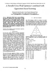
according to their average value. As for the specific formulas and the detailed calculation, please refer to literature [26]. In order to approach the best solution more quickly, the proposed algorithm in this paper improves the current best solution in solutions updating by weighting method. The update formulations are as shown in (20) and correlation coefficients are calculated by (18), (19), where 𝐴 1 , 𝐴 2 , 𝐴 3 are calculated by (16). → → → 𝐷𝛼 = 𝐶1 ⋅ 𝑋𝛼 − 𝑋⃗ , → → → (18) 𝐷𝛽 = 𝐶2 ⋅ 𝑋𝛽 − 𝑋⃗ , → → → 𝐷𝛿 = 𝐶3 ⋅ 𝑋𝛿 − 𝑋⃗ , → → → → 𝑋1 = 𝑋𝛼 − 𝐴 1 ⋅ 𝐷𝛼 , → → → → 𝑋2 = 𝑋𝛽 − 𝐴 2 ⋅ 𝐷𝛽 ,
(19)
→ → → → 𝑋3 = 𝑋𝛿 − 𝐴 3 ⋅ 𝐷𝛿 , → → → 𝑋⃗ (𝑡 + 1) = 𝑤1 ⋅ 𝑋1 + 𝑤2 ⋅ 𝑋2 + 𝑤3 ⋅ 𝑋3 ,
(20)
where 𝑤1 , 𝑤2 , 𝑤3 are the corresponding weights, which are calculated by 𝑤1 =
𝑓1 , 𝐹
𝑤2 =
𝑓2 , 𝐹
(21)
𝑓3 , 𝐹 where 𝑓1 , 𝑓2 , 𝑓3 calculated by (13) are the corresponding fitness values of 𝛼, 𝛽, 𝛿: 𝐹 = 𝑓1 +𝑓2 +𝑓3 . This paper emphasizes 𝑤3 =
that, different from GWO updating search agents, MDGWO uses (20) and (21) to update the location of search agents by weighting method for the first time; it is also the major contribution to the improved GWO. 4.3.3. Attacking Prey. The grey wolves finish the hunt by attacking the prey when it stops moving. In order to mathematically model approaching the prey, we decrease the value of 𝑒.⃗ Note that the fluctuation range of 𝐴⃗ is also decreased by 𝑒.⃗ In other words, 𝐴⃗ is a random value in the interval [−𝑒, 𝑒] where 𝑒⃗ is decreased from 2 to 0 over the course of iterations. When random values of 𝐴⃗ are in [−1, 1], the next position of a search agent can be in any position between its current position and the position of the prey; that is, the search agent will approach the best solution gradually, as shown in Figure 1. At the same time, for the purpose of mathematical model divergence, we utilize 𝐴⃗ with random values greater than 1 or less than −1 to oblige the search agent to diverge from the prey. As shown in Figure 1(b), 𝐴⃗ > 1 forces the grey wolves to diverge from the prey to hopefully find a better prey. 4.4. Pseudocode of MDGWO. The application of MDGWO algorithm in image segmentation mainly lies in optimizing Kapur’ entropy to obtain the best threshold; therefore, the fitness function as shown in (13) will be calculated based on Kapur’s entropy. Step 1. Read image 𝐽; if 𝐽 is a RGB image, then it will be processed by three channel of 𝐽R , 𝐽G , 𝐽B and store the data in ℎR , ℎG , ℎB , respectively; if 𝐽 is a grey image, then read the grey value and store it in ℎgr . Step 2. According to (3), calculate image grey values and probability distribution histogram.
Computational Intelligence and Neuroscience
7
Step 3. Initialize the population of grey wolves, parameter 𝑒,⃗ 𝐴,⃗ 𝐶,⃗ and Max iter. → Step 4. Initialize the population 𝑋𝑖 (𝑖 randomly:
=
→ 𝑋𝑖 = rand (SN, 1) ⋅ (𝑢𝑏 − 𝑙𝑏) + 𝑙𝑏.
1, 2, . . . , SN) (22)
→ Step 5. Use (11) to discretize 𝑋𝑖 , that is, being rounded toward zero. Use (12) to adjust the singular data beyond the boundaries of search space. Step 6. Calculate objective functions of each search agent by using (8). And calculate the fitness value of each search agent on the basis of objective functions. Step 7. According to the fitness values, assigning first three → → → best search agents to 𝑋𝛼 , 𝑋𝛽 , 𝑋𝛿 , respectively. → → → Step 8. Updating encircling parameters based on 𝑋𝛼 , 𝑋𝛽 , 𝑋𝛿 , → → → → → → which include calculating 𝐴 1 , 𝐴 2 , 𝐴 3 by (16), 𝐶1 , 𝐶2 , 𝐶3 by → → → (17), and 𝐷𝛼 , 𝐷𝛽 , 𝐷𝛿 by (18). Step 9. Update the position of search agents based on (19) and (20) for the next hunting. Step 10. Add one to circular point, if 𝑞 ≥ Max iter or meet the stop condition of the algorithm, the iteration will be finished and skip to Step 11; otherwise skip to Step 5. Step 11. Set the location of the wolf that has the best objective function as the best threshold of segmentation. Step 12. Input best threshold and images before and after segmentation.
5. Experiments and Discussion 5.1. Parameters Settings. The proposed algorithm has been tested under a set of benchmark images. Some of these images are widely used in the multilevel image segmentation literature to test different methods (Cameraman, Lena, Baboon, and Maize). Others are chosen on purpose from the Berkeley Segmentation Data Set and Benchmarks 500 (BSD500 for short, see [41]), as shown in Figure 2. The experiments were carried out on a Lenovo Laptop with an Intel Core i5 processor and 4 GB memory. The algorithm was developed via the signal processing toolbox, image processing toolbox, and global optimization toolbox of Matlab R2011b. According to relevant literatures, many methods were proved to have certain advantages compared with previous methods. This paper chooses the best advantageous method as comparison objective; the earlier or inferior literatures will no longer be used for the analysis. Based on quantities of contrast experiments, this paper will verify the superiority of MDGWO in image segmentation by comparison of image, data, chart, and so forth. In the following sections, MDGWO will be compared with the algorithm using electromagnetism
optimization (EMO) proposed in [20], the differential evolution (DE) [27], the Artifical Bee Colony (ABC) [10], and the original grey wolf optimizer. The EMO, DE, and ABC are the latest intelligent optimization methods by using Kapur’s entropy so far. The comparison with GWO is mainly used to test the advantages of MDWGO. In order to avoid the randomness of results, we use appropriate statistical metrics to compare the effectiveness of these algorithms. According to [19, 20] and the experiments, test thresholds are th = 2, 3, 4, 5 [1–3] and the stop criterion of each experiment is 150 iterations; the detailed settings of parameters are showed in Table 2. For verifying the stability, we use (23) to calculate the standard deviation (STD) at the end of each test. Once the STD value increases, the algorithms becomes more instable correspondingly [29]: Max iter
STD = √ ∑ 𝑖=1
2
(𝜃𝑖 − 𝜀) . Max iter
(23)
In addition, the peak signal to noise ratio (PSNR [20]) is used to compare the similarity between the segmented image and original image according to the mean square error (MSE [26]) of each pixel: PSNR = 20 log10 ( MSE = √
255 ) , (dB) , MSE
co 𝑎 𝑎 ∑ro 𝑖=1 ∑𝑗=1 (𝐼𝑜 (𝑖, 𝑗) − 𝐼th (𝑖, 𝑗))
ro × co
(24)
,
(25)
𝑎 where 𝐼𝑜𝑎 is the original image, 𝐼th is the segmented image, and 𝑎 depends on the type of image (grey image or RGB image); ro, co are, respectively, the total number of rows and columns in an image. Because Kapur’s entropy is based on histogram of the image, this paper provides test images and the corresponding histograms. From Figure 2, it can be seen that each image has the only distinctive histogram which can guarantee the universality and commonality of the algorithm. More importantly, most of these histograms do not follow the bimodal characteristic; therefore, the difficulty level of optimization increases accordingly.
5.2. The Image Segmentation Result Based on MDGWO with Different Thresholds. In order to reflect the segmentation effect, Figures 3 and 4 illustrate the segmentation results of original images in Figure 2 when the threshold is 2, 3, 4, and 5, respectively. The experiments indicate that the segmentation results turn out to be finer and there are also more segmented areas when the number of thresholds is larger and vice versa. In extreme cases, when the threshold is 2, the algorithm is reduced to be binary image segmentation (foregroundbackground segmentation). Certainly, that how many areas are segmented is related to the applications and requirements, this method only needs to set the corresponding number of thresholds (th). Besides giving the MDGWO segmentation results, like [20], Figures 3 and 4 also mark the position
8
Computational Intelligence and Neuroscience Table 2: Parameters settings of MDGWO.
Parameters Value
Population size 50
Threshold 2, 3, 4, 5
Image
Number of iterations 150
Histogram of left col.
Run time 35 Image
0.012
0.02
0.01 0.008 0.006
0.01
0.004
0.005
0.002
0 0
(a) Cameraman
50 100 150 200 250 300
0
0.008 0.006 0.004 0.002 0 0
(e) Maize
0
50 100 150 200 250 300
0
50 100 150 200 250 300
×10−3 8 7 6 5 4 3 2 1 0 0
50 100 150 200 250 300
50 100 150 200 250 300
(d) Butterfly
(f) Starfish
0.025
0.02 0.018 0.016 0.014 0.012 0.01 0.008 0.006 0.004 0.002 0
0.02 0.015 0.01 0.005 0
50 100 150 200 250 300
0.01 0.009 0.008 0.007 0.006 0.005 0.004 0.003 0.002 0.001 0
0.01
0.014 0.012 0.01 0.008 0.006 0.004 0.002 0
0
(b) Lena
0.012
(c) Baboon
Upper bound 256
Histogram of left col.
0.025
0.015
(g) Smiling Girl
Lower bound 1
0
50 100 150 200 250 300
(h) Surfing
0
50 100 150 200 250 300
Figure 2: The original images and their histograms.
of the threshold in each histogram. Compared with other MT methods, it is difficult to find the difference in terms of the segmentation effect. Therefore, Section 5.4 lists the thresholds, PSNR, STD, and MEAN for comparisons of MDGWO results and other techniques. 5.3. The Comparison of MDGWO in Multilevel Image Thresholding with Different Objective Functions. In Section 1, we summarize the relevant objective functions. The commonly used optimization functions include maximization of the entropy and maximization of the between-class variance (e.g., Otsu’s method). In [27], the authors, respectively, analyze
these objective functions and compare Kapur and Otsu systematically. The experiment results show that Kapur’s entropy gets the best effectiveness. Therefore, in order to verify MDGWO’s efficiency, we compare the thresholds and PSNR between Otsu and Kapur in Table 3. As shown in Table 3, the threshold distribution of Kapur is more dispersed and wider in most cases. However, the effect of image thresholding cannot be seen from the threshold distribution directly. Therefore, we focus on analysis the PSNR between Otsu and Kapur. In terms of PSNR, the Kapur method produces higher PSNR values on most items in Figure 2, except for the Sea Star Image with 𝑘 = 3, 5 and Surfer Image with 𝑘 = 4.
Computational Intelligence and Neuroscience
th = 2
Cameraman
Image
Lena Baboon
th = 3
th = 4
th = 5
0.025
0.025
0.025
0.02
0.02
0.02
0.02
0.015
0.015
0.015
0.015
0.01
0.01
0.01
0.01
0.005
0.005
0.005
0.005
0 0
Butterfly
9
0.012 0.01 0.008 0.006 0.004 0.002 0
0.012 0.01 0.008 0.006 0.004 0.002 0
0.01 0.009 0.008 0.007 0.006 0.005 0.004 0.003 0.002 0.001 0
0
0
0
50 100 150 200 250 300
50 100 150 200 250 300
50 100 150 200 250 300
50 100 150 200 250 300
0
0.012 0.01 0.008 0.006 0.004 0.002 0
0.012 0.01 0.008 0.006 0.004 0.002 0
0.01 0.009 0.008 0.007 0.006 0.005 0.004 0.003 0.002 0.001 0
0
0
0
0
50 100 150 200 250 300
50 100 150 200 250 300
50 100 150 200 250 300
50 100 150 200 250 300
0
0.012 0.01 0.008 0.006 0.004 0.002 0
0.012 0.01 0.008 0.006 0.004 0.002 0
0.01 0.009 0.008 0.007 0.006 0.005 0.004 0.003 0.002 0.001 0
0.025
0
0
0
0
50 100 150 200 250 300
50 100 150 200 250 300
50 100 150 200 250 300
50 100 150 200 250 300
0
0.012 0.01 0.008 0.006 0.004 0.002 0
0.012 0.01 0.008 0.006 0.004 0.002 0
0.01 0.009 0.008 0.007 0.006 0.005 0.004 0.003 0.002 0.001 0
0
50 100 150 200 250 300
0
50 100 150 200 250 300
0
50 100 150 200 250 300
0
50 100 150 200 250 300
Figure 3: The segmentation results of (a)–(d) in Figure 2 and their thresholds in histograms.
10
Computational Intelligence and Neuroscience th = 2
Surfing
Smiling Girl
Starfish
Maize
Image
0.014 0.012 0.01 0.008 0.006 0.004 0.002 0
0
50 100 150 200 250 300
×10−3 8 7 6 5 4 3 2 1 0 0 50 100 150 200 250 300
th = 3
0.014 0.012 0.01 0.008 0.006 0.004 0.002 0
0
50 100 150 200 250 300
×10−3 8 7 6 5 4 3 2 1 0 0 50 100 150 200 250 300
th = 4
0.014 0.012 0.01 0.008 0.006 0.004 0.002 0
0
50 100 150 200 250 300
×10−3 8 7 6 5 4 3 2 1 0 0 50 100 150 200 250 300
th = 5
0.014 0.012 0.01 0.008 0.006 0.004 0.002 0
0.025
0.025
0.025
0.02
0.02
0.02
0.02
0.015
0.015
0.015
0.015
0.01
0.01
0.01
0.01
0.005
0.005
0.005
0.005
0
0
0
0.02 0.018 0.016 0.014 0.012 0.01 0.008 0.006 0.004 0.002 0
0
50 100 150 200 250 300
50 100 150 200 250 300
0.02 0.018 0.016 0.014 0.012 0.01 0.008 0.006 0.004 0.002 0
0
0
50 100 150 200 250 300
50 100 150 200 250 300
0.02 0.018 0.016 0.014 0.012 0.01 0.008 0.006 0.004 0.002 0
0
0
50 100 150 200 250 300
50 100 150 200 250 300
50 100 150 200 250 300
×10−3 8 7 6 5 4 3 2 1 0 0 50 100 150 200 250 300
0.025
0
0
0
0.02 0.018 0.016 0.014 0.012 0.01 0.008 0.006 0.004 0.002 0
0
50 100 150 200 250 300
0
50 100 150 200 250 300
Figure 4: The segmentation results of (e)–(h) in Figure 2 and their thresholds in histograms.
Computational Intelligence and Neuroscience
11
Table 3: The comparison of MDGWO’s efficiency between Otsu and Kapur. Image
Cameraman
Lena
Baboon
Butterfly
Maize
Sea Star
Smiling Girl
Surfer
𝑘
Otsu thresholds
2 3
70 58
144 119
156
4 5
40 35
93 81
139 121
2 3 4
92 80 75
151 126 114
171 145
180
136
161
170 149
5
73
109
2 3 4
97 83 70
149 123 105
160 136
167
5
66
98
125
150
2
100
152
3 4
81 73
118 101
159 129
164
121
149
5
69
95
2
92
168
3 4 5
76 65 56
128 104 86
187 150 123
2 3
85 69
157 120
178
4 5
59 51
99 85
137 117
2 3
60 47
123 100
131
4 5
28 20
74 63
111 95
2 3
92 71
162 111
177
4 5
47 46
81 77
118 105
200 164
187 150
136 124
179 143
PSNR
174
189
175
177
208
193
158
196
The average value of Kapur is improved averagely by 22.24% compared to Otsu by checking against the corresponding PSNR values which are obtained from the MDGWO. The maximum value is increased by 53.42% for Cameraman Image when 𝑘 = 3. Therefore, the Kapur method is significantly better than the Otsu method, and we also mainly analyze the effectiveness of Kapur’s method in Section 5.4. 5.4. The Comparison of Quality Assessment by PSNR, STD, and MEAN. This paper adopts PSNR standard to evaluate the segmentation quality in comparison with other MT methods. Tables 4–6 illustrate the PSNR values under different thresholds of MDGWO, GWO, EMO, DE, ABC, and the MEAN and STD of objective functions. As shown in Table 4, it can be
Kapur thresholds
11.9475 12.9933
44 44
106 98
148
16.0180 16.3710
39 23
83 58
119 94
13.1029 15.7626 16.4291
93 70 43
163 121 81
172 127
171
103
141
PSNR 14.4629 19.9337
156 125
16.7206
41
73
12.4396 13.7731 14.9493
78 46 34
141 103 75
151 117
159
16.0012
29
64
100
134
12.4400
87
150
14.2563 14.6987
62 49
104 88
152 128
168
113
145
159
21.1684 23.1191 14.7164 17.5144 20.1729
178
21.8208 16.0302 18.6340 20.5198
170
22.0929 14.9325
16.4688
48
80
13.6677
84
165
15.2676 16.7309 18.5649
59 45 39
113 80 74
171 125 108
14.8445 17.6040
81 60
160 111
172
19.4039 21.4000
46 47
89 83
131 118
13.1358 12.8470
88 44
145 91
145
15.6914 18. 2260
24 44
67 83
100 115
12.5401 16.0569
52 52
141 103
168
20.8786 21.6071
49 24
86 53
131 88
18.5539 21.0711 180
22.4539 14.0407
187 147
198
16.5853 18.9818 20.8792 14.8595 17.4583
184 150
196
19.4487 20.9681 18.0033 19.1148
145 152
203
20.0759 21.7937 16.4343 18.9343
185 126
183
20.7218 21.8961
seen from the PSNR values that MDGWO gets the highest evaluation in most cases. Thus, it proves that MDGWO gets better results on image segmentation. In addition, when the number of thresholds increases, it shows superior PSNR value. In detail, the MDGWO algorithm produces higher PSNR values on all items in Table 4 except for the Smiling Girl Image with 𝑘 = 5 and Surfer Image with 𝑘 = 4 on the result of DE. As shown in Table 4, the average value of MDGWO is improved averagely by 13.16% compared to GWO by checking against the corresponding PSNR values. The maximum value is increased by 45.05% for Butterfly Image when 𝑘 = 5. Comparing with MTEMO, the average value of MDGWO is improved averagely by 11.56% by checking against the corresponding PSNR values. The maximum value is increased by 39.94% for Surfer Image when 𝑘 = 2.
12
Computational Intelligence and Neuroscience Table 4: PSNR metrics of MTEMO, DE, ABC, GWO, and MDGWO.
Image
Cameraman
Lena
Baboon
Butterfly
Maize
Sea Star
Smiling Girl
Surfer
𝑘
MTEMO
DE
ABC
GWO
MDGWO
2 3
13.626 18.803
12.584 17.584
13.920 14.462
14.279 19.696
14.463 19.934
4 5
20.586 20.661
20.111 21.282
20.81 22.40
20.809 22.404
21.168 23.119
2 3 4
14.672 17.247 18.251
8.823 14.386 16.151
14.590 17.197 18.559
14.680 17.416 19.762
14.716 17.514 20.173
5
20.019
16.720
20.321
21.299
21.820
2 3 4
16.016 16.016 18.485
8.103 12.596 13.178
16.007 18.592 18.417
16.024 18.632 20.480
16.035 18.634 20.519
5
20.507
13.135
20.224
22.060
22.092
2
11.065
8.702
14.402
14.762
14.932
3 4
14.176 16.725
13.028 13.028
14.504 16.189
17.873 21.021
18.553 21.071
5
19.026
14.786
19.286
21.485
22.453
2
13.633
10.549
13.590
13.950
14.040
3 4 5
15.229 16.280 17.211
13.022 14.270 15.079
15.295 16.346 17.046
16.201 18.713 20.410
16.585 18.981 20.879
2 3
14.398 16.987
8.610 14.078
14.395 16.981
14.809 17.431
14.885 17.458
4 5
18.304 20.165
16.191 16.474
18.427 20.330
19.421 20.887
19.448 20.968
2 3
13.420 18.254
14.986 11.243
13.514 18.069
17.989 18.742
18.003 19.114
4 5
18.860 19.840
14.556 22.980
18.826 19.769
19.823 21.214
20.075 21.793
2 3
11.744 18.584
9.737 11.638
11.878 18.762
16.154 18.895
16.434 18.934
4 5
19.478 20.468
21.866 19.576
19.647 20.479
20.234 21.699
20.721 21.896
By comparing with DE, the average value of MDGWO is improved averagely by 38.14% by checking against the corresponding PSNR values. The maximum value is increased by 97.89% for Baboon Image when 𝑘 = 2. The PSNR of the Smiling Girl with 𝑘 = 5 and Surfer Image with 𝑘 = 4 are slightly lower, but the gap is not significant. Comparing between ABC and MDGWO, the average value of MDGWO is improved averagely by 10.55% by checking against the corresponding PSNR values. The maximum value is increased by 38.36% for Surfer Image when 𝑘 = 2. From the perspective of STD which is shown in Table 5, it can be observed that MDGWO shows obviously advantages over MTEMO, DE, ABC, and GWO. The smaller the STD is, the smaller the change of fitness functions over the course of iterations will be, that is, the better stability of segmentation.
Therefore, the results show that MDGWO obtains exciting effect in stability. So MDGWO’s stability is better. Compared with GWO, the average value of MDGWO is improved averagely by 73.52% compared to GWO by checking against the corresponding STD values. The maximum value is increased by 96.44% for Baboon Image when 𝑘 = 3, and the minimum value is increased by 24.92% for Baboon Image when 𝑘 = 3. By comparing with MTEMO, the average value of MDGWO is improved averagely by 47.88%. The maximum value is increased by 87% for Lena Image when 𝑘 = 2, and the minimum value is increased by 0.6% for Surfer Image when 𝑘 = 3. Comparing between DE and MDGWO, the average value of MDGWO is improved averagely by 95.60%. The maximum
Computational Intelligence and Neuroscience
13
Table 5: STD metrics of MTEMO, DE, ABC, GWO, and MDGWO. Image
Camerman
Lena
Baboon
Butterfly
Maize
Sea Star
Smiling Girl
Surfer
𝑘
MTEMO
DE
ABC
GWO
MDGWO
2 3
0.1849 0.1649
1.2592 1.7601
0.1235 0.2122
0.1697 0.2287
0.0462 0.0758
4 5
0.2943 0.2999
2.1995 2.6579
0.3003 0.2784
0.3627 0.4278
0.0659 0.1964
2 3 4
0.0969 0.1665 0.2800
1.2902 1.7822 2.2104
0.0349 0.1300 0.1872
0.1536 0.3570 0.5965
0.0126 0.0264 0.0939
5
0.2515
2.5992
0.1827
0.5946
0.1570
2 3 4
0.0108 0.0393 0.1727
1.2862 1.7678 2.2126
0.0358 0.0202 0.1610
0.2171 0.4376 0.2986
0.0102 0.0156 0.1184
5
0.2868
2.6239
0.2660
0.5377
0.2316
2
0.0903
1.2708
0.0750
0.2179
0.0465
3 4
0.2207 0.2482
1.7429 2.2368
0.2952 0.3906
0.2712 0.4808
0.2036 0.2415
5
0.2900
2.6571
0.4818
0.5096
0.2684
2
0.0356
1.3501
0.0218
0.3571
0.0188
3 4 5
0.1222 0.2305 0.2502
1.8612 2.3230 2.7461
0.0901 0.2605 0.3834
0.2225 0.3903 0.4584
0.0270 0.0927 0.1677
2 3
0.1073 0.1497
1.3547 1.8741
0.1088 0.1752
0.1728 0.2028
0.0290 0.0374
4 5
0.1596 0.2639
2.3307 2.7550
0.1817 0.2180
0.5032 0.4550
0.1119 0.1437
2 3
0.0377 0.0955
1.2516 1.7311
0.0318 0.0577
0.1834 0.1712
0.0111 0.0242
4 5
0.1966 0.1550
2.1878 2.5989
0.1094 0.2768
0.2508 0.5273
0.0781 0.1302
2 3
0.0579 0.1002
1.3213 1.8337
0.0303 0.1646
0.2681 0.3014
0.0245 0.0996
4 5
0.3382 0.3690
2.3317 2.7846
0.1686 0.2580
0.3162 0.3815
0.1424 0.1706
value is increased by 99.21% for Baboon Image when 𝑘 = 2. The minimum value is increased by 88.32% for Butterfly Image when 𝑘 = 3. Comparing with ABC, the average value of MDGWO is improved averagely by 45.90%. The maximum value is increased by 79.70% for Lena Image when 𝑘 = 3, and the minimum value is increased by 12.93% for Baboon Image when 𝑘 = 5. As far as MEAN is concerned, this parameter presents the average value of fitness function over the course of iterations in Table 6, which reflects the algorithm stability to some extent. But its accuracy of evaluation is relatively low which can only reflect the fuzzy stability of the algorithm. The experiment data is offered here just in response to the parameter provided in literature [20]. In comparison with GWO, MTEWO, DE, and ABC in Table 6, it can be safely
assumed that, in most cases, MDGWO obtains higher MEAN of fitness function. Moreover, the difference is extremely small when MDGWO’s MEAN is lower. From the analyses of Tables 3–6, together with the visual effects of Figures 2, 3, and 4, it can be observed that MDGWO method obtains better segmentation effect and has advantage in optimal process, accuracy, stability, and robustness. Therefore, MDGWO is a MT algorithm with high accuracy and high segmentation quality.
6. Conclusion This paper proposes a modified discrete grey wolf optimizer, which is used to optimize the image histograms and realize the multilevel image segmentation. Based on the high efficiency of GWO in the course of optimization and stability,
14
Computational Intelligence and Neuroscience Table 6: MEAN metrics of MTEMO, DE, ABC, GWO, and MDGWO.
Image Camerman
Lena
Baboon
Butterfly
Maize
Sea Star
Smiling Girl
Surfer
𝑘 2 3 4 5 2 3 4 5 2 3 4 5 2 3 4 5 2 3 4 5 2 3 4 5 2 3 4 5 2 3 4 5
MTEMO 17.584 21.976 26.586 30.506 17.831 22.120 25.999 29.787 17.625 22.269 26.688 30.800 16.681 21.242 25.179 28.611 18.631 23.565 27.529 31.535 18.754 23.323 27.582 31.562 17.334 21.904 26.040 30.089 18.339 23.231 27.863 31.823
DE 12.4212 17.3764 21.7520 26.2505 12.7730 17.6428 21.8784 25.7311 12.7333 17.5005 21.9010 25.9681 12.5796 17.2545 22.0176 26.1795 13.3566 18.4245 22.9813 27.1709 13.4104 18.5516 23.0719 27.2551 12.3892 17.1339 21.6541 25.7130 13.0786 18.1492 23.0548 27.4979
this paper successfully applies the MDGWO to the field of MT by improving the location selection mechanism of 𝛼, 𝛽, and 𝛿 during the hunting and using weight to optimize the final position of prey (best threshold). The MDGWO method not only obtains better segmentation quality but also shows obvious superiority over GWO, MTEMO, DE, and ABC in stability, accuracy, and multilevel thresholding.
Competing Interests The authors declare that there are no competing interests regarding the publication of this paper.
Acknowledgments This work was supported in part by the National Natural Science Foundation of China (no. 61300239, no. 71301081, and no. 61572261), the Postdoctoral Science Foundation (no.
ABC 17.7638 22.3059 26.8409 30.8328 17.8139 22.0832 26.0615 29.9664 17.6760 22.1276 26.3912 30.3464 17.4205 22.2209 26.3794 30.6533 18.6316 23.2496 27.3931 31.2127 18.7295 23.2738 27.5057 31.4919 17.3129 21.8601 25.9904 30.0225 18.3393 23.2889 27.8017 31.7335
GWO 14.634 21.107 24.927 30.436 17.809 22.074 25.318 29.252 17.679 22.129 26.194 30.067 17.425 21.585 25.267 29.492 18.604 22.941 26.936 31.023 18.321 23.245 27.136 31.167 17.136 21.253 25.050 29.870 18.283 23.243 27.275 31.384
MDGWO 17.471 21.919 27.480 30.548 18.396 22.856 26.447 30.381 18.619 22.949 26.900 30.076 17.723 22.498 26.190 29.899 19.542 23.939 27.842 30.694 19.587 23.901 28.210 31.958 18.035 21.980 26.597 30.574 18.869 24.135 27.447 31.325
2014M551635 and no. 1302085B), the Innovation Project of Graduate Students Foundation of Jiangsu Province (KYLX15 0841), the Higher Education Revitalization Plan Foundation of Anhui Province (no. 2013SQRL102ZD, no. 2015xdjy196, no. 2015jyxm728, no. 2016jyxm0774, and no. 2016jyxm0777), and Natural Science Fund for Colleges and Universities in Jiangsu Province (no.16KJB520034), A Project Funded by the Priority Academic Program Development of Jiangsu Higher Education Institutions (PAPD), and Jiangsu Collaborative Innovation Center on Atmospheric Environment and Equipment Technology (CICAEET).
References [1] M. Sonka, V. Hlavac, and R. Boyle, Image Processing, Analysis, and Machine Vision, Cengage Learning, 2014. [2] S. Masood, M. Sharif, A. Masood, M. Yasmin, and M. Raza, “A survey on medical image segmentation,” Current Medical Imaging Reviews, vol. 11, no. 1, pp. 3–14, 2015.
Computational Intelligence and Neuroscience [3] P. Ghamisi, M. S. Couceiro, F. M. L. Martins, and J. A. Benediktsson, “Multilevel image segmentation based on fractional-order darwinian particle swarm optimization,” IEEE Transactions on Geoscience and Remote Sensing, vol. 52, no. 5, pp. 2382–2394, 2014. [4] M. Waseem Khan, “A survey: image segmentation techniques,” International Journal of Future Computer and Communication, vol. 3, no. 2, pp. 89–93, 2014. [5] J. Li, X. Li, B. Yang, and X. Sun, “Segmentation-based image copy-move forgery detection scheme,” IEEE Transactions on Information Forensics and Security, vol. 10, no. 3, pp. 507–518, 2015. [6] Z. Pan, J. Lei, Y. Zhang, X. Sun, and S. Kwong, “Fast motion estimation based on content property for low-complexity H.265/HEVC encoder,” IEEE Transactions on Broadcasting, vol. 62, no. 3, pp. 675–684, 2016. [7] X. Chen, S. Feng, and D. Pan, “An improved approach of lung image segmentation based on watershed algorithm,” in Proceedings of the the 7th International Conference on Internet Multimedia Computing and Service, pp. 1–5, Zhangjiajie, China, August 2015. [8] Y. Zheng, B. Jeon, D. Xu, Q. M. J. Wu, and H. Zhang, “Image segmentation by generalized hierarchical fuzzy C-means algorithm,” Journal of Intelligent and Fuzzy Systems, vol. 28, no. 2, pp. 961–973, 2015. [9] V. Osuna-Enciso, E. Cuevas, and H. Sossa, “A comparison of nature inspired algorithms for multi-threshold image segmentation,” Expert Systems with Applications, vol. 40, no. 4, pp. 1213– 1219, 2013. [10] T. Kurban, P. Civicioglu, R. Kurban, and E. Besdok, “Comparison of evolutionary and swarm based computational techniques for multilevel color image thresholding,” Applied Soft Computing Journal, vol. 23, pp. 128–143, 2014. [11] J. N. Kapur, P. K. Sahoo, and A. K. C. Wong, “A new method for gray-level picture thresholding using the entropy of the histogram,” Computer Vision, Graphics, and Image Processing, vol. 29, no. 3, pp. 273–285, 1985. [12] N. Otsu, “A threshold selection method from gray-level histograms,” Automatica, vol. 11, no. 285–296, pp. 23–27, 1975. [13] X. Li, Z. Zhao, and H. D. Cheng, “Fuzzy entropy threshold approach to breast cancer detection,” Information Sciences Applications, vol. 4, no. 1, pp. 49–56, 1995. [14] J. Kittler and J. Illingworth, “Minimum error thresholding,” Pattern Recognition, vol. 19, no. 1, pp. 41–47, 1986. [15] Y. Xue, S. Zhong, T. Ma, and J. Cao, “A hybrid evolutionary algorithm for numerical optimization problem,” Intelligent Automation & Soft Computing, vol. 21, no. 4, pp. 473–490, 2015. [16] P.-Y. Yin, “A fast scheme for optimal thresholding using genetic algorithms,” Signal Processing, vol. 72, no. 2, pp. 85–95, 1999. [17] W. Fujun, L. Junlan, L. Shiwei, Z. Xingyu, Z. Dawei, and T. Yanling, “An improved adaptive genetic algorithm for image segmentation and vision alignment used in microelectronic bonding,” IEEE/ASME Transactions on Mechatronics, vol. 19, no. 3, pp. 916–923, 2014. [18] S. Banerjee and N. D. Jana, “Bi level kapurs entropy based image segmentation using particle swarm optimization,” in Proceedings of the 3rd International Conference on Computer, Communication, Control and Information Technology (C3IT ’15), pp. 1–4, Hooghly, India, February 2015. [19] M.-H. Horng, “Multilevel thresholding selection based on the artificial bee colony algorithm for image segmentation,” Expert Systems with Applications, vol. 38, no. 11, pp. 13785–13791, 2011.
15 [20] D. Oliva, E. Cuevas, G. Pajares, D. Zaldivar, and V. Osuna, “A multilevel thresholding algorithm using electromagnetism optimization,” Neurocomputing, vol. 139, pp. 357–381, 2014. [21] S. Sarkar, G. R. Patra, and S. Das, “A differential evolution based approach for multilevel image segmentation using minimum cross entropy thresholding,” in Swarm, Evolutionary, and Memetic Computing, pp. 51–58, Springer, Berlin, Germany, 2011. [22] Y. Xue, Y. Zhuang, T. Ni, S. Ni, and X. Wen, “Self-adaptive learning based discrete differential evolution algorithm for solving CJWTA problem,” Journal of Systems Engineering and Electronics, vol. 25, no. 1, pp. 59–68, 2014. [23] S. Agrawal, R. Panda, S. Bhuyan, and B. K. Panigrahi, “Tsallis entropy based optimal multilevel thresholding using cuckoo search algorithm,” Swarm and Evolutionary Computation, vol. 11, pp. 16–30, 2013. [24] P. D. Sathya and R. Kayalvizhi, “Optimal multilevel thresholding using bacterial foraging algorithm,” Expert Systems with Applications, vol. 38, no. 12, pp. 15549–15564, 2011. [25] S. Ayas, H. Dogan, E. Gedikli, and M. Ekinci, “Microscopic image segmentation based on firefly algorithm for detection of tuberculosis bacteria,” in Proceedings of the 23rd Signal Processing and Communications Applications Conference (SIU ’15), pp. 851–854, Malatya, Turkey, May 2015. [26] S. Mirjalili, S. M. Mirjalili, and A. Lewis, “Grey wolf optimizer,” Advances in Engineering Software, vol. 69, pp. 46–61, 2014. [27] B. Akay, “A study on particle swarm optimization and artificial bee colony algorithms for multilevel thresholding,” Applied Soft Computing, vol. 13, no. 6, pp. 3066–3091, 2013. [28] A. K. Bhandari, A. Kumar, and G. K. Singh, “Modified artificial bee colony based computationally efficient multilevel thresholding for satellite image segmentation using Kapur’s, Otsu and Tsallis functions,” Expert Systems with Applications, vol. 42, no. 3, pp. 1573–1601, 2015. [29] P. Ghamisi, M. S. Couceiro, J. A. Benediktsson, and N. M. F. Ferreira, “An efficient method for segmentation of images based on fractional calculus and natural selection,” Expert Systems with Applications, vol. 39, no. 16, pp. 12407–12417, 2012. [30] L. Li, L. Sun, W. Kang, J. Guo, C. Han, and S. Li, “Fuzzy multilevel image thresholding based on modified discrete grey wolf optimizer and local information aggregation,” IEEE Access, vol. 4, pp. 6438–6450, 2016. [31] H.-S. Wu, F.-M. Zhang, and L.-S. Wu, “New swarm intelligence algorithm-wolf pack algorithm,” Xi Tong Gong Cheng Yu Dian Zi Ji Shu/Systems Engineering and Electronics, vol. 35, no. 11, pp. 2430–2438, 2013. [32] H. Wu and F. Zhang, “A uncultivated wolf pack algorithm for high-dimensional functions and its application in parameters optimization of PID controller,” in Proceedings of the IEEE Congress on Evolutionary Computation (CEC ’14), pp. 1477–1482, Beijing, China, July 2014. [33] H.-S. Wu and F.-M. Zhang, “Wolf pack algorithm for unconstrained global optimization,” Mathematical Problems in Engineering, vol. 2014, Article ID 465082, 17 pages, 2014. [34] Q. Zhou and Y. Zhou, “Wolf colony search algorithm based on leader strategy,” Application Research of Computers, vol. 9, pp. 2629–2632, 2013. [35] G. M. Komaki and V. Kayvanfar, “Grey Wolf Optimizer algorithm for the two-stage assembly flow shop scheduling problem with release time,” Journal of Computational Science, vol. 8, pp. 109–120, 2015.
16 [36] L. I. Wong, M. H. Sulaiman, M. R. Mohamed, and M. S. Hong, “Grey Wolf Optimizer for solving economic dispatch problems,” in Proceedings of the IEEE International Conference on Power and Energy (PECon ’14), pp. 150–154, Kuching, Malaysia, December 2014. [37] A. Chaman-Motlagh, “Superdefect photonic crystal filter optimization using Grey Wolf Optimizer,” IEEE Photonics Technology Letters, vol. 27, no. 22, pp. 2355–2358, 2015. [38] P. Q. Dzung, N. T. Tien, N. Dinh Tuyen, and H. Lee, “Selective harmonic elimination for cascaded multilevel inverters using grey wolf optimizer algorithm,” in Proceedings of the 9th International Conference on Power Electronics and ECCE Asia (ICPE ’15-ECCE Asia), June 2015. [39] N. Muangkote, K. Sunat, and S. Chiewchanwattana, “An improved grey wolf optimizer for training q-Gaussian Radial Basis Functional-link nets,” in Proceedings of the International Computer Science and Engineering Conference (ICSEC ’14), pp. 209–214, Khon Kaen, Thailand, August 2014. [40] A. Zhu, C. Xu, Z. Li, J. Wu, and Z. Liu, “Hybridizing grey Wolf optimization with differential evolution for global optimization and test scheduling for 3D stacked SoC,” Journal of Systems Engineering and Electronics, vol. 26, no. 2, pp. 317–328, 2015. [41] P. Arbel´aez, M. Maire, C. Fowlkes, and J. Malik, “Contour detection and hierarchical image segmentation,” IEEE Transactions on Pattern Analysis and Machine Intelligence, vol. 33, no. 5, pp. 898–916, 2011.
Computational Intelligence and Neuroscience
Journal of
Advances in
Industrial Engineering
Multimedia
Hindawi Publishing Corporation http://www.hindawi.com
The Scientific World Journal Volume 2014
Hindawi Publishing Corporation http://www.hindawi.com
Volume 2014
Applied Computational Intelligence and Soft Computing
International Journal of
Distributed Sensor Networks Hindawi Publishing Corporation http://www.hindawi.com
Volume 2014
Hindawi Publishing Corporation http://www.hindawi.com
Volume 2014
Hindawi Publishing Corporation http://www.hindawi.com
Volume 2014
Advances in
Fuzzy Systems Modelling & Simulation in Engineering Hindawi Publishing Corporation http://www.hindawi.com
Hindawi Publishing Corporation http://www.hindawi.com
Volume 2014
Volume 2014
Submit your manuscripts at https://www.hindawi.com
Journal of
Computer Networks and Communications
Advances in
Artificial Intelligence Hindawi Publishing Corporation http://www.hindawi.com
Hindawi Publishing Corporation http://www.hindawi.com
Volume 2014
International Journal of
Biomedical Imaging
Volume 2014
Advances in
Artificial Neural Systems
International Journal of
Computer Engineering
Computer Games Technology
Hindawi Publishing Corporation http://www.hindawi.com
Hindawi Publishing Corporation http://www.hindawi.com
Advances in
Volume 2014
Advances in
Software Engineering Volume 2014
Hindawi Publishing Corporation http://www.hindawi.com
Volume 2014
Hindawi Publishing Corporation http://www.hindawi.com
Volume 2014
Hindawi Publishing Corporation http://www.hindawi.com
Volume 2014
International Journal of
Reconfigurable Computing
Robotics Hindawi Publishing Corporation http://www.hindawi.com
Computational Intelligence and Neuroscience
Advances in
Human-Computer Interaction
Journal of
Volume 2014
Hindawi Publishing Corporation http://www.hindawi.com
Volume 2014
Hindawi Publishing Corporation http://www.hindawi.com
Journal of
Electrical and Computer Engineering Volume 2014
Hindawi Publishing Corporation http://www.hindawi.com
Volume 2014
Hindawi Publishing Corporation http://www.hindawi.com
Volume 2014