Jun 20, 2018 - Degree Distance, Modified Generalized Degree Distance, Graph Operations. 1. Introduction. Throughout this paper all graphs considered are ...
Advances in Pure Mathematics, 2018, 8, 548-558 http://www.scirp.org/journal/apm ISSN Online: 2160-0384 ISSN Print: 2160-0368
Modified Generalized Degree Distance of Some Graph Operations Shengmei Lv School of Mathematics and Statistics, Qinghai Nationalities University, Xining, China
How to cite this paper: Lv, S.M. (2018) Modified Generalized Degree Distance of Some Graph Operations. Advances in Pure Mathematics, 8, 548-558. https://doi.org/10.4236/apm.2018.86032 Received: May 3, 2018 Accepted: June 17, 2018 Published: June 20, 2018 Copyright © 2018 by author and Scientific Research Publishing Inc. This work is licensed under the Creative Commons Attribution International License (CC BY 4.0). http://creativecommons.org/licenses/by/4.0/ Open Access
Abstract The modified generality degree distance, is defined as:
H λ* ( G ) =
∑
d λ ( u , v ) ( dG ( u ) dG ( v ) ) , which is a modification of the ge-
{u ,v}⊆V ( G )
nerality degree distance. In this paper, we give some computing formulas of the modified generality degree distance of some graph operations, such as, composition, join, etc.
Keywords Degree Distance, Modified Generalized Degree Distance, Graph Operations
1. Introduction Throughout this paper all graphs considered are finite and simple graphs. Let G
be such a graph with vertex set V ( G ) and edge set E ( G ) , and denoted by
n and m the values of V ( G )
and
E ( G ) , respectively. For vertices
u , v ∈ V ( G ) , the distance between u and v in G, denoted by dG ( u , v ) , is the
length of a shortest
( u, v ) -path in G, and let
dG ( v ) be the degree of a vertex
v ∈ V ( G ) . The complement of G, denoted by G , is the graph with vertex set
V ( G ) , in which two distinct vertices are adjacent if and only if they are not ad-
( )
jacent in G, and denoted by m the value of E G . We use Cn , Pn and K n to denote the cycle, path and complete graph on n vertices, respectively. Other terminology and notation will be introduced where it is needed or can be found in [1]. A Topological index of a graph is a real number related to the graph; it does not depend on labeling or pictorial representation of a graph. In chemistry, topological index is used for modeling physicochemical, pharmacologic, biological and other properties of chemical compounds [2]. One of the oldest and DOI: 10.4236/apm.2018.86032 Jun. 20, 2018
548
Advances in Pure Mathematics
S. M. Lv
well-studied distance-based graph invariants is the Wiener number W ( G ) , also termed as Wiener index in chemical or mathematical chemistry literature, which is defined [3] as the sum of distances over all unordered vertex pairs in G, namely, W (G ) =
∑
dG ( u, v ) .
{u ,v}⊆V ( G )
Dobrynin and Kochetova [4] and Gutman [5] introduced a new graph invariant with the name degree distance or Schultz molecular topological index, which is defined as follows:
∑ ( dG ( u ) + dG ( v ) ) dG ( u, v ) .
= DD ( G )
{u ,v}⊆V ( G )
In [6], Gutman and Klavzar defined product-degree distance as follow:
= DD∗ ( G )
∑ ( dG ( u ) ⋅ dG ( v ) ) dG ( u, v ) .
{u ,v}⊆V ( G )
Note that the degree distance and product-degree distance are degree-weight versions of the Wiener index. We encourage the interested readers to consult [7] [8] [9] for Wiener index. In [4] [10] [11] [12] [13] [14], there are more conclusions for degree distance, which shows that the research of degree distance is a hot topic. In [15], Sagan et al. computed some exact formulae for the Wiener polynomial of various graph operations containing Cartesian product, composition, join, disjunction and symmetric difference of graphs, whose concepts will be presented in later part. In [16], Hamzeh et al. consider the generalized degree distances of some graph operations. The generalized degree distance of a graph is defined as follow [17]:
= Hλ (G )
∑
d λ ( u, v ) ( dG ( u ) + dG ( v ) ) .
{u ,v}⊆V ( G )
(1)
For a real number λ , the modified generalized degree distance, denoted by H λ* ( G ) , is also defined in [17]:
H λ* ( G ) =
∑
d λ ( u, v ) ( dG ( u ) dG ( v ) ) .
{u ,v}⊆V ( G )
(2)
If λ = 0 , H λ ( G ) = 4m and H λ* ( G ) = 4m 2 . When λ = 1 , H λ ( G ) = DD ( G ) and H λ* ( G ) = DD* ( G ) , which implies that the generalized degree distance is equal to the degree distance (or Schultz index), and the modified generalized degree distance is equal to the product-degree distance. Therefore the study of this new topological index is important and we try to obtain some new results related to this topological index.
In this paper, we show that the explicit formulas for H λ* ( G ) of some graph
operations containing the composition, join, disjunction and symmetric difference of graphs, and we apply the results to compute the modified generality degree distance of some special graphs. Next, we introduce four types of graph operations: The join G = G1 + G2 of graphs G1 and G2 with disjoint vertex sets V1 , DOI: 10.4236/apm.2018.86032
549
Advances in Pure Mathematics
S. M. Lv
V2 and edge sets E1 , E2 is the graph union G1 G2 together with all the edges joining V1 and V2 .
The composition G = G1 [G2 ] of graphs G1 and G2 with disjoint vertex
sets V1 and V2 and edge sets E1 and E2 is the graph with vertex set V1 × V2
and u = ( u1 , v1 ) is adjacent with v = ( u2 , v2 ) whenever ( u1 is adjacent with
u2 ) or ( u1 = u2 and v1 is adjacent with v2 ), see [18]. The disjunction G ∨ H of graphs G and H is the graph with vertex set
V ( G ) × V ( H ) and
or v1v2 ∈ E ( H ) .
( u1 , v1 )
is adjacent with
( u2 , v2 )
whenever u1u2 ∈ E ( G )
The symmetric difference G ⊕ H of two graphs G and H is the graph with
vertex set V ( G ) × V ( H ) and
= E (G ⊕ H )
{( u1 , u2 )( v1 , v2 ) | u1v1 ∈ E ( G ) or u2v2 ∈ E ( H ) but not both} .
In the final of this section, we present several well-known indices: the first
Zagreb index M 1 ( G ) and the second Zagreb index M 2 ( G ) [19], the first
Zagreb conindex M 1 ( G ) and the second Zagreb coindex M 2 ( G ) [20], which will be used in our results.
= M1 ( G )
= M 2 (G )
∑
dG ( u= ) , M1 ( G ) 2
u∈V ( G )
∑ ( dG ( u ) + dG ( v ) ) .
uv∈ / E(G )
= ∑ ( dG ( u ) dG ( v ) ) , M 2 ( G )
uv∈E ( G )
∑ ( dG ( u ) dG ( v ) ) .
uv∈/E ( G )
In fact, M 1 ( G ) can be also expressed as a sum over edges of G,
= M1 ( G )
∑ ( dG ( u ) + dG ( v ) ) .
uv∈E ( G )
2. Main Results The purpose of this section is to compute the modified generalized degree distance for four graph operations. We begin with the following crucial lemma related to distance properties of some graph operations. Lemma 2.1. [18] [21] Let G and H be two graphs, then we have:
1) V ( G ∨ H ) = V ( G [ H ]) = V ( G ⊕ H ) = V ( G ) ⋅ V ( H ) , 2
2
E ( G ∨ H )= E ( G ) ⋅ V ( H ) + E ( H ) ⋅ V ( G ) − 2 E ( G ) ⋅ E ( H ) , E ( G + H )=
E (G ) + E ( H ) + V (G ) ⋅ V ( H ) , 2
2
E ( G ⊕ H )= E ( G ) ⋅ V ( H ) + E ( H ) ⋅ V ( G ) − 4 E ( G ) ⋅ E ( H ) , E ( G [ H ]) = E ( G ) ⋅ V ( H ) + E ( H ) ⋅ V ( G ) . 2
2) The join, composition, disjunction and symmetric difference of graphs are associative and all of them are commutative except from composition. 0 u=v uv ∈ E ( G ) or uv ∈ E ( H ) or ( u ∈ V ( G ) & V ∈ V ( H ) ) 3) dG + H ( u , v ) =1 otherwise, 2 DOI: 10.4236/apm.2018.86032
550
Advances in Pure Mathematics
S. M. Lv
d G ( a, c ) a ≠ c = a c= &b d 0 4) dG[ H ] ( ( a, b ) , ( c, d ) ) = = a c & bd ∈ E ( H ) 1 2 = a c & bd ∈/ E ( H ) , &b d a c= 0 = 5) dG∨ H ( ( a, b ) , ( c, d ) ) = ac ∈ E ( G ) or bd ∈ E ( H ) 1 2 otherwise, &b d a c= 0 = 6) dG⊕ H ( ( a, b ) , ( c, d ) ) = 1 ac E ∈ ( G ) or bd ∈ E ( H ) but not both 2 otherwise, dG ( a ) + V ( H ) 7) dG + H ( a ) = d H ( a ) + V ( G )
a ∈V (G ) a ∈V ( H )
,
8) = dG[ H ] ( ( a, b ) ) V ( H ) dG ( a ) + d H ( b ) , 9) dG⊕ H ( ( a, b ) ) = V ( H ) dG ( a ) + V ( G ) d H ( b ) − 2dG ( a ) d H ( b ) , 10) dG∨ H ( ( a, b ) ) = V ( H ) dG ( a ) + V ( G ) d H ( b ) − dG ( a ) d H ( b ) . Proof. The parts 1) - 5) are consequence of definitions and some well-known results of the book of Imrich and Klavzar [18]. For the proof of 6) - 10) we refer to [21].
■
For a given graph Gi , we denote ni and mi by the number of vertices and edges, respectively. Then we can obtain the modified generalized degree distance of the join graph G1 + G2 as following: Theorem 2.1. Let G1 and G2 be two graphs. Then
H λ* ( G = 2λ ( n2 M 1 ( G1 ) + n1M 1 ( G2 ) + M 2 ( G1 ) + M 2 ( G2 ) ) 1 + G2 )
(
)
+ 2λ n22 m1 + n12 m2 + n2 M 1 ( G1 ) + n1M 1 ( G2 ) + M 2 ( G1 ) + M 2 ( G2 ) + 4m1m2 + n1n2 ( 2m1 + n1n2 + 2m2 ) + n22 m1 + n12 m2 . Proof. In the graph G1 + G2 , we can partition the set of pairs of vertices of
G1 + G2 into three subsets A1 , A2 and A3 . In A1 , we collect all pairs of vertices u and v such that u is in G1 and v is in G2 . Hence, they are adjacent in
G1 + G2 . The sets A2 and A3 are the set of pairs of vertices u and v which are in G1 and G2 , respectively. Therefore, we can partition the sum in the formu-
la of H λ* ( G1 + G2 ) into three sums Si such that Si is over Ai for i = 1, 2,3 . By 3) and 7) of Lemma 2.1, we have
= S1*
∑ ∑
((
dGλ1+G2 ( u , v ) dG1 ( u ) + n2
u∈V ( G1 ) v∈V ( G2 )
)(d
G2
( v ) + n1 ) )
= 4m1m2 + n2 n2 ( 2m1 + n1n2 + 2m2 ) .
= S2* =
∑
((
dGλ1+G2 ( u , v ) dG1 ( u ) + n2
{u ,v}⊆V ( G1 )
)(d
G1
( v ) + n2 ) )
∑ ( ( dG ( u ) + n2 ) ( dG ( v ) + n2 ) ) + ∑
uv∈E ( G1 )
1
1
(
)
uv∈ / E ( G1 )
2λ
(( d
G1
( u ) + n2 ) ( dG ( v ) + n2 ) ) 1
= 2λ M 2 ( G1 ) + n2 M 1 ( G1 ) + n22 m1 + M 2 ( G1 ) + n2 M 1 ( G1 ) + n22 m1. DOI: 10.4236/apm.2018.86032
551
Advances in Pure Mathematics
S. M. Lv
= S3* =
∑
((
)(
dGλ1+G2 ( u , v ) dG2 ( u ) + n1 dG2 ( v ) + n1
{u ,v}⊆V ( G2 )
∑ ( ( dG ( u ) + n1 ) ( dG ( v ) + n1 ) ) + ∑
uv∈E ( G2 )
2
2
(
)
uv∈ / E ( G2 )
2λ
))
(( d
G2
( u ) + n1 ) ( dG ( v ) + n1 ) ) 2
= 2λ M 2 ( G2 ) + n1M 1 ( G2 ) + n12 m2 + M 2 ( G2 ) + n1M 1 ( G2 ) + n12 m2 . Therefore,
H λ* ( G1 + G2 ) = S1* + S2* + S3*
(
= 2λ ( n2 M 1 ( G1 ) + n1M 1 ( G2 ) + M 2 ( G1 ) + M 2 ( G2 ) ) + 2λ n22 m1 + n12 m2
)
+ n2 M 1 ( G1 ) + n1M 1 ( G2 ) + M 2 ( G1 ) + M 2 ( G2 ) + 4m1m2 + n1n2 ( 2m1 + n1n2 + 2m2 ) + n22 m1 + n12 m2 . ■ In the above theorem, if λ = 1 , then we can obtain DD ( G1 + G2 ) . Replace *
separately G1 and G2 by K1 and G in Theorem 2.1, we can obtain the following result. Corollary 2.2. Let G be a connected graph with n vertices and m edges. Then H λ* ( K= 2λ ( M 1 ( G ) + M 2 ( G ) + m ) + ( M 1 ( G ) + M 2 ( G ) ) + n 2 + 2nm + m. 1 + G)
We can observe that M 1 ( Cn ) = 4n for n ≥ 3 , M 1 ( Pn= ) 4n − 6 for n > 1 ,
and M 1 (= = 2 ( n − 2 ) . Hence, we can compute the Cn ) 2 n ( n − 3 ) , M 1 ( P n) 2
formulae for modified generalized degree distance of fan graph K1 + Pn and wheel graph K1 + Cn (see Figure 1) in the following. Example 2.1. H λ* ( K1 += Pn ) 2λ −1 9n 2 − 39n + 44 + 3n 2 + 7 n − 15 .
(
) (
)
H λ* ( K1 += Cn ) 2λ −19n ( n − 3) + 3n ( n + 3) . Next, we compute the exact formula for the modified generalized degree distance of the composition of two graphs. Before starting the discussion, we first denote by A ( G ) the sum
∑ ii≠, jj=1dGλ ( ui , u j ) dG ( ui ) . It is easy to deduce that n
d ( u , u ) d ( u ) = ∑ d ( ui , u j ) dG ( u j ) . By calculations we obtain the expressions for A ( Pn ) and A ( Cn ) as follow-
∑
n n λ λ i, j 1 = i, j 1 G = G i j G i i≠ j i≠ j
ing:
A (= Pn )
n −1
∑ 2 ( 2n − 2i − 1) i λ , i =1
Figure 1. The graphs Pn + K1 and Cn + K1 . DOI: 10.4236/apm.2018.86032
552
Advances in Pure Mathematics
S. M. Lv
n2−1 λ ∑ i=1 4ni , A ( Cn ) = n −2 21−λ n1+λ + ∑ i=21 4ni λ ,
n is odd, n is even.
we can also obtain the expressions for H λ* ( Pn ) and H λ* ( Cn ) : n −1
H λ* ( Pn ) = 2 ( n − 1) + ∑8 ( i − 1)( n − i ) . λ
λ
i =2
n2−1 λ n is odd, ∑ i=1 8ni , H λ* ( Cn ) = λ n −2 4n n + ∑ 2 8ni λ , n is even. i =1 2
These formulae are similar to the known results in [22]: n −1
n −1
Wλ= ( Pn ) n∑i λ − ∑i λ +1 , =i 1 =i 1
n −1 λ n∑ i=21 i , Wλ ( Cn ) = λ +1 n−2 n + n∑ 2 i λ , i =1 2
n is odd, n is even.
Theorem 2.3. Let G1 and G2 be two graphs. Then
(
= H λ* ( G1 [G 2λ n22 m2 M 1 ( G1 ) + n1M 2 ( G2 ) + 2n2 m1M 1 ( G2 ) 2 ])
)
+ 2n2 ( m2 M 1 ( G1 ) + m1M 1 ( G2 ) ) + n1M 2 ( G2 ) + 4n22 m2 A ( G1 ) + 4m22Wλ ( G1 ) + n24 H λ* ( G1 ) .
{
}
{
}
Proof. Set V ( G1 ) = u1 , u2 , , un1 and V ( G2 ) = v1 , v2 , , vn2 . By 4), 8) of Lemma 2.1 and definition of H λ* ( G ) , we have
(
H λ* ( G1 [G2 ]) = ∑ {u ,v}⊆V ( G [G ])dGλ1[G2 ] ( u , v ) dG1[G2 ] ( u ) dG1[G2 ] ( v ) 1 2 =
)
1 ∑ ∑ d λ ( ui , vk ) , ( u j , vl ) n2 dG1 ( ui ) + dG2 ( vk ) 2 ( ui ,vk ) ( u j ,vl ) G1[G2 ]
(
(
)(
)
) ] ((u , v ) , (u , v )) ( n d (u ) + n d (u )
⋅ n2 dG1 ( u j ) + dG2 ( vl ) =
∑ p=1∑ k ,l =1 n1
n2
dGλ1[G2
vk vl ∈E ( G2 )
(
p
k
p
)
⋅ dG2 ( vk ) + dG2 ( vl ) + dG2 ( vk ) dG2 ( vl )
(
2 2 2 G1
l
p
2 G1
p
)
)(
+ ∑ k2,l =1∑ i ,1j =1dGλ1[G2 ] ( ui , vk ) , ( u j , vl ) n22 dG1 ( ui ) dG1 ( u j ) n
n
i≠ j
+ n2 dG1 ( ui ) dG2 ( vl ) + n2 dG1 ( u j ) dG2 ( vk ) + dG2 ( vk ) dG2 ( vl ) + ∑ p=1∑ n1
n2 λ k ,l =1 G1[G2 ] vk vl ∈ / E ( G2 )
d
(
((u , v ) , (u , v )) ( n d (u ) i
k
j
l
2 2 2 G1
p
)
+ n2 dG1 ( u p ) dG2 ( vk ) + dG2 ( vl ) + dG2 ( vk ) dG2 ( vl )
(
)
)
)
= 2λ n22 m2 M 1 ( G1 ) + n1M 2 ( G2 ) + 2n2 m1M 1 ( G2 ) + 2n2 ( m2 M 1 ( G1 ) + m1M 1 ( G2 ) ) + n1M 2 ( G2 ) + 4n m2 A ( G1 ) + 4m22Wλ ( G1 ) + n24 H λ* ( G1 ) 2 2
■ DOI: 10.4236/apm.2018.86032
553
Advances in Pure Mathematics
S. M. Lv
In Theorem 2.3, H λ* ( G1 [G2 ]) = DD* ( G1 [G2 ]) if λ = 1 , and in the above
(
))
(
proof, when = ui u j & vk vl ∈ E ( G2 ) , dG1[G2 ] ( ui , vk ) , u j , vl = 1 ; when ui ≠ u j , dG1[G2 ] ( ui , vk ) , u j , vl = dG1 ui , u j ; when = ui u j & vk vl ∈ / E ( G2 ) , dG1[G2 ] ( ui , vk ) , u j , vl = 2 by Lemma 2.1 4).
( (
)) ))
( (
(
)
By composing paths or cycles with various small graphs, we can obtain classes
of polymer-like graphs. As an application, we give the formulae of H λ* ( Pn [ K 2 ])
and H λ* ( Cn [ K 2 ]) , where Pn [ K 2 ] and Cn [ K 2 ] are open fence graph and closed fence graph (see Figure 2), respectively.
(
)
Example 2.2. H λ* ( Pn [ K 2 ]) = 25n − 32 + 24 H λ* ( Pn ) + A ( Pn ) + 4Wλ ( Pn ) ,
(
)
H λ ( Cn [ K 2 ]= ) 25n − 8 + 2 H λ ( Cn ) + A ( Cn ) + 4Wλ ( Cn ) . *
4
*
The following theorem characterizes the modified generalized degree distance of the disjunction of two graphs. Theorem 2.4. Let G1 and G2 be two graphs. Then
H λ* ( G1 ∨ G2 )
( (
)
(
)
= 2λ n2 n22 + 2n2 m2 − 4m2 M 2 ( G1 ) + n1 n12 + 2n1m1 − 4m1 M 2 ( G2 ) + n m2 M 1 ( G1 ) + n m1M 1 ( G2 ) + 2n1n2 ( m2 M 1 ( G1 ) + m1M 1 ( G2 ) ) 2 2
+ 2λ
2 1
(( M (G ) − n M (G )) M 1
2
2
1
2
2
)
( G1 ) + ( M1 ( G1 ) − n1M1 ( G1 ) ) M 2 ( G2 )
+ ( n1n2 M 1 ( G1 ) M 1 ( G2 ) − n1M 1 ( G1 ) M 1 ( G2 ) − n2 M 1 ( G2 ) M 1 ( G1 ) )
(
)
+ M 2 ( G1 ) M 2 ( G2 ) ) + 4n22 m12 m2 + 4n12 m22 m1 + 2n1m2 n22 − 2m2 M 1 ( G1 )
(
)
(
)(
)
+ 2n2 m1 n12 − 2m1 M 1 ( G2 ) + n22 − m2 n22 − 4m2 M 2 ( G1 )
(
)(
)
+ n12 − m1 n12 − 4m1 M 2 ( G2 ) − n1n2 M 1 ( G1 ) M 1 ( G2 ) + n1M 1 ( G1 ) M 2 ( G2 ) + n2 M 1 ( G2 ) M 2 ( G1 ) − M 2 ( G1 ) M 2 ( G2 ) . Proof. By the definition of G1 ∨ G2 , we first present the following four sums:
Figure 2. The graphs Pn [ K 2 ] and Cn [ K 2 ] . DOI: 10.4236/apm.2018.86032
554
Advances in Pure Mathematics
S. M. Lv
∑{x, y}⊆V (G )∑ uv∈E (G ) ( n2 dG ( x ) + n1dG ( u ) − dG ( x ) dG ( u ) )
= S1*
1
1
2
2
1
(
⋅ n2 dG1 ( y ) + n1dG2 ( v ) − dG1 ( y ) dG2 ( v ) 2 2 G1
2
1
+ ∑{x , y}⊆V ( G )∑ uv∈E ( G ) n d 1
2 1 G2
2
)
( x ) dG ( y )
= ∑{x , y}⊆V ( G )∑ uv∈E ( G ) n d 1
2
( u ) dG ( v ) 2
(
+ ∑{x , y}⊆V ( G )∑ uv∈E ( G ) n1n2 dG1 ( x ) dG2 ( v ) + dG1 ( y ) dG2 ( u ) 1
2
( (v ) ⋅ ( d
)
) ( y ))
− ∑ {x , y}⊆V ( G )∑ uv∈E( G ) n2 dG1 ( x ) dG1 ( y ) dG2 ( u ) + dG2 ( v ) 1
2
− ∑ {x , y}⊆V ( G )∑ uv∈E( G ) n1dG2 ( u ) dG2 1
2
1
2
( x ) + dG ( u ) dG ( v )
+ ∑ {x , y}⊆V ( G )∑ uv∈E( G ) dG1 ( x ) dG1 ( y ) dG2
(
)
G1
1
2
(
= 4n22 m12 m2 + 2n2 m1 n12 − 2m1 M 1 ( G2 ) + n12 − 2m1
)
2
M 2 ( G2 )
∑ xy∈E(G )∑ {u ,v}⊆V (G ) ( n2 dG ( x ) + n1dG ( u ) − dG ( x ) dG ( u ) )
= S2*
1
(
1
2
2
⋅ n2 dG1 ( y ) + n1dG2 ( v ) − dG1 ( y ) dG2 ( v )
1
2
)
= ∑ xy∈E( G )∑ {u ,v}⊆V ( G ) n22 dG1 ( x ) dG1 ( y ) 1
2
+ ∑ xy∈E( G )∑ {u ,v}⊆V ( G ) n12 ⋅ dG2 ( u ) dG2 ( v ) 1
2
(
+ ∑ xy∈E( G )∑ {u ,v}⊆V ( G ) n1n2 dG1 ( x ) dG2 ( v ) + dG1 ( y ) dG2 ( u ) 1
2
(
)
) ( y ))
− ∑ xy∈E( G )∑ {u ,v}⊆V ( G ) n2 dG1 ( x ) dG1 ( y ) dG2 ( u ) + dG2 ( v ) 1
2
(
− ∑ xy∈E( G )∑ {u ,v}⊆V ( G ) n1dG2 ( u ) dG2 ( v ) ⋅ dG1 ( x ) + dG1 1
2
+ ∑ xy∈E( G )∑ {u ,v}⊆V ( G ) dG1 ( x ) dG1 ( y ) dG2 ( u ) dG2 ( v ) 1
2
(
)
(
= 4n m m1 + 2n1m2 n − 2m2 M 1 ( G1 ) + n22 − 2m2 2 1
2 2
2 2
)
2
M 2 ( G1 )
∑ xy∈E(G )∑ uv∈E(G ) ( n2 dG ( x ) + n1dG ( u ) − dG ( x ) dG ( u ) )
= S3*
1
(
1
2
2
1
⋅ n2 dG1 ( y ) + n1dG2 ( v ) − dG1 ( y ) dG2 ( v ) = ∑ xy∈E( G )∑ uv∈E( G ) n d 1
2 2 G1
2
+ ∑ xy∈E( G )∑ uv∈E( G ) n d 1
2
2
)
( x ) dG ( y ) 1
2 1 G2
( u ) dG ( v ) 2
(
+ ∑ xy∈E( G )∑ uv∈E( G ) n1n2 dG1 ( x ) dG2 ( v ) + dG1 ( y ) dG2 ( u ) 1
2
( (v) (d
)
) ( y ))
− ∑ xy∈E( G )∑ uv∈E( G ) n2 dG1 ( x ) dG1 ( y ) dG2 ( u ) + dG2 ( v ) 1
2
− ∑ xy∈E( G )∑ uv∈E( G ) n1dG2 ( u ) dG2 1
2
1
2
+ ∑ xy∈E( G )∑ uv∈E( G ) dG1 ( x ) dG1 ( y ) dG2
( x ) + dG ( u ) dG ( v ) G1
1
2
= n m2 M 2 ( G1 ) + n1n2 M 1 ( G1 ) M 1 ( G2 ) − n2 M 1 ( G2 ) M 2 ( G1 ) 2 2
+ n12 m1M 2 ( G2 ) − n1M 1 ( G1 ) M 2 ( G2 ) + M 2 ( G1 ) M 2 ( G2 )
S4* =
∑ xyx≠∈/yE(G )∑ uvu≠∈/vE(G )2λ ( n2 dG ( x ) + n1dG ( u ) − dG ( x ) dG ( u ) ) 1
2
1
(
2
⋅ n2 dG1 ( y ) + n1dG2 ( v ) − dG1 ( y ) dG2 ( v )
(
1
2
)
+ ∑ xy∈/ E( G )∑ u∈V ( G ) 2λ n2 dG1 ( x ) + n1dG2 ( u ) − dG1 ( x ) dG2 ( u ) 1
DOI: 10.4236/apm.2018.86032
2
555
)
Advances in Pure Mathematics
S. M. Lv
⋅ n2 dG1 ( y ) + n1dG2 ( v ) − dG1 ( y ) dG2 ( v )
(
)
+ ∑ x∈V ( G )∑ uv∈/E( G ) 2
2
(
1
λ
2
(n d
2 G1
( x ) + n1dG ( u ) − dG ( x ) dG ( u ) )
⋅ n2 dG1 ( y ) + n1dG2 ( v ) − dG1 ( y ) dG2 ( v )
= 2λ
(( n
3 2
)
(
1
2
)
)
+ 2n22 m2 − 4n2 m2 M 2 ( G1 ) + n13 + 2n12 m1 − 4n1m1 M 2 ( G2 )
+ 2n1n2 ( m2 M 1 ( G1 ) + m1 M 1 ( G2 ) ) + n12 m1 M 1 ( G2 ) + n22 m2 M 1 ( G1 ) + 2λ
(( n n M 1 2
1
)
( G1 ) M1 ( G2 ) − n1M 1 ( G2 ) M 1 ( G1 ) − n2 M 1 ( G1 ) M 1 ( G2 ) )
+ ( M 1 ( G2 ) − n2 M 1 ( G2 ) ) M 2 ( G1 ) + ( M 1 ( G1 ) − n1 M 1 ( G1 ) ) M 2 ( G2 )
)
+ 2 M 2 ( G1 ) M 2 ( G2 ) . λ
Thus, we can obtain the result of Theorem 2.4 by the formula H λ* ( G1 ∨ G2 ) = S1* + S2* + S4* − S3* . ■ Finally, we consider the modified generalized degree distance of the symmetric difference of two graphs. Theorem 2.5. Let G1 and G2 be two graphs. Then
H λ* ( G1 ⊕ G2 )
( (
)
(
)
= 2λ n2 n22 + 2n2 m2 − 8m2 M 2 ( G1 ) + n1 n12 + 2n1m1 − 8m1 M 2 ( G2 ) + n22 m2 M 1 ( G1 ) + n12 m1M 1 ( G2 ) + 2n1n2 ( m2 M 1 ( G1 ) + m1M 1 ( G2 ) )
( 2 ( 2M ( G ) − n M ( G ) ) M
)
( G1 ) + 2 ( 2M1 ( G1 ) − n1M1 ( G1 ) ) M 2 ( G2 ) + n1n2 M 1 ( G1 ) M 2 ( G2 ) − 2n1M 1 ( G1 ) M 1 ( G2 ) − 2n2 M 1 ( G2 ) M 1 ( G1 ) + 22 M 2 ( G1 ) M 2 ( G2 ) ) + 4n22 m12 m2 + 4n12 m22 m1 + 2n1m2 ( n22 − 4m2 ) M 1 ( G1 ) +2
λ
1
2
(
2
1
2
)
2
(
+ 2n2 m1 n12 − 4m1 M 1 ( G2 ) + n22 − 2m2
(
)(
)( n
)
− 8m2 M 2 ( G1 )
2 2
)
+ n12 − 2m1 n12 − 8m1 M 2 ( G2 ) − 2n1n2 M 1 ( G1 ) M 1 ( G2 ) + 4n1 M 1 ( G1 ) M 2 ( G2 ) + 4n2 M 1 ( G2 ) M 2 ( G1 ) − 8M 2 ( G1 ) M 2 ( G2 ) . Proof. Similar to the proof of Theorem 2.4, we consider four sums:
= S1*
∑{x, y}⊆V (G )∑ uv∈E (G ) ( n2 dG ( x ) + n1dG ( u ) − dG ( x ) dG ( u ) ) 1
(
1
2
2
1
2
) = 4n m m + 2n m ( n − 4m ) M ( G ) + ( n − 4m ) M ( G ) . = S ∑ ( ) ∑{ } ( ) ( n d ( x ) + n d ( u ) − d ( x ) d ( u ) ) ⋅ ( n d ( y ) + n d ( v ) − d ( y ) d ( v )) = 4n m m + 2n m ( n − 4m ) M ( G ) + ( n − 4m ) M ( G ) . S = ∑ ( )∑ ( ) ( n d ( x ) + n d ( u ) − d ( x ) d ( u ) ) ⋅ ( n d ( y ) + n d ( v ) − d ( y ) d ( v )) ⋅ n2 dG1 ( y ) + n1dG2 ( v ) − dG1 ( y ) dG2 ( v ) 2 2
* 2
2 1
2
xy∈E G1
2
* 3
2 2
2 1
1
1 G2
1
xy∈E G1 2 G1
1
2
uv∈E G2
1 G2
1
2 G1
u , v ⊆V G2
2 G1
2 1
1
2
2 G1
1
2
G1
2
G2
G2
1
1
1 G2
G1
2
2 1
1 G2
G1
2 2
2
2
2 2
2
G1
2
1
G2
G2
= n m2 M 2 ( G1 ) + n1n2 M 1 ( G1 ) M 1 ( G2 ) − 2n2 M 1 ( G2 ) M 2 ( G1 ) 2 2
+ n12 m1 M 2 ( G2 ) − 2n1 M 1 ( G1 ) M 2 ( G2 ) + 4 M 2 ( G1 ) M 2 ( G2 ) . DOI: 10.4236/apm.2018.86032
556
Advances in Pure Mathematics
S. M. Lv
= S4*
∑ xyx≠∈/yE(G )∑ uuv≠∈/vE(G )2λ ( n2 dG ( x ) + n1dG ( u ) − dG ( x ) dG ( u ) ) 1
(
2
1
2
⋅ n2 dG1 ( y ) + n1dG2 ( v ) − dG1 ( y ) dG2 ( v ) = 2
λ
(( n
3 2
)
(
1
2
)
)
+ 2n m2 − 8n2 m2 M 2 ( G1 ) + n + 2n12 m1 − 8n1m1 M 2 ( G2 ) 2 2
3 1
+ 2n1n2 ( m2 M 1 ( G1 ) + m1M 1 ( G2 ) ) + n12 m1M 1 ( G2 ) + n22 m2 M 1 ( G1 ) + 2λ
(( n n M 1 2
1
)
( G1 ) M 1 ( G2 ) − 2n1M 1 ( G2 ) M 1 ( G1 ) − 2n2 M 1 ( G1 ) M 1 ( G2 ) )
+ 2 ( 2 M 1 ( G2 ) − n2 M 1 ( G2 ) ) M 2 ( G1 ) + 2 ( 2 M 1 ( G1 ) − n1 M 1 ( G1 ) ) M 2 ( G2 ) +2
λ +2
)
M 2 ( G1 ) M 2 ( G2 ) .
Therefore, we can obtain the result of Theorem 2.5 by H λ* ( G1 ⊕ G2 ) = S1* + S2* + S4* − 2 S3* .
■
Remark. In Section 2, we present the explicit formulae of the modified generalized degree distance for four types of graph operations containing G1 + G2 , G1 [G2 ] , G1 ∨ G2 and G1 ⊕ G2 , and we give some examples. It implies that our
results are convenient to compute the modified generalized degree distance of these graph operations. Moreover, if λ = 1 , then H λ* ( G ) = DD* ( G ) . This im-
plies that our results are related to the product-degree distance. In [16] Hamzeh
et al. construct graph polynomial as following: H λ* ( G, x ) =
d ∑ ( dG ( u ) dG ( v ) ) x
{u ,v}⊆V ( G )
λ
( u ,v )
.
It is easy to see that the results of our Theorems 2.1, 2.3, 2.4 and 2.5 are exactly
the first derivatives at point x = 1 of the graph polynomial H λ* ( G, x ) . Thus we
obtain the relation between the modified generalized degree distance polynomial and Wiener-type invariant polynomial for graphs.
Funding This work is supported by the National Natural Science Foundation of China (11761056) and by Natural Science Foundation of Qinghai Province (2018-ZJ-717), and by the Fund of Qinghai Nationalities University (2016XJG08).
References
DOI: 10.4236/apm.2018.86032
[1]
Bondy, J. and Murty, U. (1976) Graph Theory with Applications. Elsevier, New York. https://doi.org/10.1007/978-1-349-03521-2
[2]
Gutman, I. and Polansky, O. (1986) Mathematical Concepts in Organic Chemistry. Springer-Verlag, Berlin. https://doi.org/10.1007/978-3-642-70982-1
[3]
Wiener, H. (1947) Structural Determination of Paraffin Boiling Point. Journal of the American Chemical Society, 69, 17-20. https://doi.org/10.1021/ja01193a005
[4]
Dobrynin, A. and Kochetova, A. (1994) Degree Distance of a Graph: A Degree Analogue of the Wiener Index. Journal of Chemical Information and Computer Sciences, 34, 1082-1086. https://doi.org/10.1021/ci00021a008
[5]
Gutman, I. (1994) Selected Properties of the Schultz Molecular Topogical Index. Journal of Chemical Information and Computer Sciences, 34, 1087-1089. https://doi.org/10.1021/ci00021a009 557
Advances in Pure Mathematics
S. M. Lv [6]
Gutman, I. and Klavzarć, S. (1997) Wiener Number of Vertex-Weighted Graphs and a Chemical Applications. Discrete Applied Mathematics, 80, 73-81. https://doi.org/10.1016/S0166-218X(97)00070-X
[7]
Gutman, I. (1997) A Property of the Wiener Number and Its Modifications. Indian Journal of Chemistry: Section A, 36, 128-132.
[8]
Gutman, I., Rada, J. and Araujo, O. (2000) The Wiener Index of Starlike Trees and a Related Partial Order. MATCH Communications in Mathematical and in Computer Chemistry, 42, 145-154.
[9]
Hua, H. (2009) Wiener and Schultz Molecular Topological Indices of Graphs with Specified Cut Edges. MATCH Communications in Mathematical and in Computer Chemistry, 16, 643-651.
[10] Dankelmann, P., Gutman, I., Mukwembi, S. and Swart, H.C. (2009) On the Degree Distance of a Graph. Discrete Applied Mathematics, 157, 2773-2777. https://doi.org/10.1016/j.dam.2009.04.006 [11] Feng, L., Liu, W., Ili, A. and Yu, G. (2013) Degree Distance of Unicyclic Graphs with Given Matching Number. Graphs and Combinatorics, 5, 449-462. https://doi.org/10.1007/s00373-012-1143-5 [12] Ilić, A., Stevanović, D., Feng, L., Yu, G. and Dankelmann, P. (2011) Degree Distance of Unicyclic and bicyclic Graphs. Discrete Applied Mathematics, 159, 779-788. https://doi.org/10.1016/j.dam.2011.01.013 [13] Tomescu, I. (2008) Properties of Connected Graphs Having Minimum Degree Distance. Discrete Math, 309, 2745-2748. https://doi.org/10.1016/j.disc.2008.06.031 [14] Tomescu, I. (2010) Ordering Connected Graphs Having Small Degree Distances. Discrete Applied Mathematics, 158, 1714-1717. https://doi.org/10.1016/j.dam.2010.05.023 [15] Sagan, B., Yeh, Y. and Zhang, P. (1996) The Wiener Polynomial of a Graph. International Journal of Quantum Chemistry, 60, 959-969. https://doi.org/10.1002/(SICI)1097-461X(1996)60:53.0.CO;2-W [16] Hamzeh, A., Iranmanesh, A. and Hossein-Zadeh, S. (2013) Some Results on Generalized Degree Distance. Open Journal of Discrete Mathematics, 3, 143-150. https://doi.org/10.4236/ojdm.2013.33026 [17] Hamzeh, A., Iranmanesh, A., Hossein-Zadeh, S. and Diudea, M. (2012) Generalized Degree Distance of Trees, Unicyclic and Bicyclic Graphs. Studia Universitatis Babeș-Bolyai. Chemia, 4, 73-85. [18] Imrich, W. and Klavzarć, S. (2000) Product Graphs: Structure and Recognition. John Wiley & Sons, New York. [19] Gutman, I. and Trinajstic, N. (1972) Graph Theory and Molecular Orbitals. Total φ-Electron Energy of Alternant Hydrocarbons. Chemical Physics Letters, 17, 535-538. https://doi.org/10.1016/0009-2614(72)85099-1 [20] Došlić, T. (2008) Vertex-Weighted Wiener Polynomials for Composite Graphs. Ars Mathematica Contemporanea, 1, 66-80. [21] Khalifeh, M., Yousefi-Azari, H. and Ashrafi, A. (2008) The Hyper-Wiener Index of Graph Operations. Computers & Mathematics with Applications, 56, 1402-1407. https://doi.org/10.1016/j.camwa.2008.03.003 [22] Hossein-Zadeh, S., Hamzeh, A. and Ashrafi, A. (2009) Wiener-Type Invariants of Some Graph Operations. Filomat, 29, 103-113. https://doi.org/10.2298/FIL0903103H
DOI: 10.4236/apm.2018.86032
558
Advances in Pure Mathematics