Modified Naïve Bayes Classifier for E-Catalog Classification∗ Young-gon Kim1, Taehee Lee1, Jonghoon Chun2, and Sang-goo Lee1 1
School of Computer Science and Engineering / Center for E-Business Research Seoul National University, Seoul 151-742, Republic of Korea {gumory, thlee, sglee}@europa.snu.ac.kr 2 Department of Computer Engineering Myongji University, 449-728, Yongin, Kyunggi-Do, Republic of Korea
[email protected]
Abstract. As the wide use of online business transactions, the volume of product information that needs to be managed in a system has become drastically large, and the classification task of such data has become highly complex. The heterogeneity among competing standard classification schemes makes the problem only harder. However, the classification task is an indispensable part for successful e-commerce applications. In this paper, we present an automated approach for e-catalog classification. We extend the Naïve Bayes Classifier to make use of the structural characteristics of e-catalogs. We show how we can improve the accuracy of classification when appropriate characteristics of ecatalogs are utilized. Effectiveness of the proposed methods is validated through experiments.
1 Introduction E-catalog (Electronic catalog) hold information of products and services in an ecommerce system. E-catalog classification is the task of assigning an input catalog to one of the predefined categories (or classes). The categories are defined according to a specific classification scheme which usually has a hierarchical structure and thousands of leaf nodes. Correct classification is essential not only for data alignment and synchronization among business partners but also to keep the rapidly increasing product data maintainable and accessible. However, product data classification is a highly time-consuming task when it is done manually because of the increased scale of product information and the inherent complexity of the classification schemes. A number of competing standard classification schemes, such as UNSPSC1 and eCl@ss, do exist nowadays. Since none of them has yet been accepted universally, we need to reclas∗ This work was supported by the Ministry of Information & Communications, Korea, under the Information Technology Research Center (ITRC) Support Program. 1 http://www.unspsc.org J. Lee et al. (Eds.): DEECS 2006, LNCS 4055, pp. 246 – 257, 2006. © Springer-Verlag Berlin Heidelberg 2006
Modified Naïve Bayes Classifier for E-Catalog Classification
247
sify the product data for mapping between different classification schemes as a part of business operations [1]. The reclassification task increases the need for an automated approach for product data classification. E-catalogs are text intensive documents, so text classification techniques can be applied to e-catalog classification. Works in [2] applied several techniques from information retrieval and machine learning to product data classification. Among the well known algorithms such as Vector Space Model, k-Nearest Neighbor, and Naïve Bayes Classifier, they report that the Naïve Bayes Classifier shows the best accuracy. Although there is no single standard form of the e-catalog, conceptually it is a set of attribute-value pairs which, in turn, can be viewed as a structured document. Motivated by the intuition that the structural nature can be utilized, we shift our attention to making a structure-aware Naïve Bayes Classifier. When the Naïve Bayes Classifier is used for flat text classification, each word position is defined to be an attribute of the Naïve Bayes Classifier [3, 4]. Our approach differs from [3, 4] since our objective is to classify a set of attribute-value pairs instead. We start from the conventional Naïve Bayes Classifier rather than the textoriented model in order to make use of the attribute-wise distribution of the terms. Furthermore, noticing that each attribute has different discriminative power, we treat individual attributes differently by assigning weights according to their importance. In order to assign weights to the attributes in a reasonable way, we normalize attributes before weighting. We further improve the classification accuracy by utilizing the ‘category name’ attribute which is available in the training data. Our classifier shows improved accuracy compared to the Naïve Bayes Text Classifier especially in the real data which possibly have noisy attributes. The remainder of this paper is organized as follows. In section 2, we investigate the related work. In section 3, we describe how we modify conventional Naïve Bayes Classifier to make it applicable for e-catalog classification. In section 4, we present the implementation of our classifier and in section 5, we present experimental results. Finally in section 6, we conclude this paper.
2 Related Work Recently, with the rapid growth of semi-structured documents their classification issue has attracted an increasing attention. The common motivation is that the structure of documents may contain useful information for classification. In [5], terms in a document are augmented with tags. For example, in an XML document John Doe..., the term 'John' is augmented to yield 'resume.name.John'. Using these augmented terms, the Naive Bayes Classifier shows fairly improved accuracy. The classifier in [6] is based on the Bayesian networks. For each document in the training set, it constructs a Bayesian network whose structure is the same as that of the document itself (a hierarchically structured document can be modeled as a tree). The conditional probabilities collected from these Bayesian networks are used to infer the category of an input document which is also represented as a Bayesian network. Works in [7] present a way of building a rule based classifier for
248
Y.-g. Kim et al.
XML documents and [8] suggests a Bayesian network based classifier which classifies structured multimedia documents. [9], which has just been published online, presents similar model to ours. It splits a semi-structured document into parts according to the structure of the document and builds a separate classifier, level-0 classifier, for each part. Then the result of each level-0 classifier serves as an input to the metaclassifier which combines the inputs to finally determine the category. In comparison, our work takes simpler approach where the entire process is done in a single classifier by using a predetermined weighting policy to assign normalized weights for different attributes. By designing an efficient weight determining method, we expect that our model can be effectively used for general structured document classification.
3 Customized Naïve Bayes Classifier for E-Catalog Classification The Naïve Bayes Classifier has a long successful application history in the field of text classification due to its favorable space and speed complexity and relatively good performance. In this section, we illustrate the process of customizing the Naïve Bayes Classifier for e-catalog classification. 3.1 Naïve Bayes Classifier To classify an instance d, the Naïve Bayes Classifier calculates the posterior probability P(c|d) based on the Bayes Theorem and the independence assumption. Given a set of classes C, the attributes < a1 , a2 , L , an > and the values < v1 , v2 , L, vn > that describe an input instance, the Naïve Bayes Classifier assigns the most probable category according to the following formula.
c NB = arg max P(c j )∏ P( ai = vi | c j ) c j ∈C
i
(1)
Conceptually, this model classifies an instance which consists of a set of attributevalue pairs. If we try to use this classifier to diagnose a disease, proper attributes may be age, sex, blood pressure, etc. and the domains of the attributes must be totally different. When this model is applied to text classification, each word position is defined as an attribute. Given a list of words < w1 , w2 , L, wn > that constitutes an input document,
c NB = arg max P(c j )∏ P(ai = wi | c j ) c j ∈C
i
(2)
In this formula, the domain of each attribute is assumed to be the same. To reduce the computation cost, we can make an additional assumption that the attributes are identically distributed, which means that the probability of encountering a specific word is independent of the specific word position [4]. This is quite reasonable for flat text classification but clearly wrong for structured document classification. Most of the
Modified Naïve Bayes Classifier for E-Catalog Classification
249
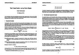
adaptations of Naïve Bayes Classifier for text classification are based on this formula. The classifiers introduced in Sect. 2, [5] and [6], also start from this model although they use their own techniques to take advantage of the structural information. In contrast, we start from the model described by Eq. (1), the original Naïve Bayes Classifier. The attributes are those of e-catalog. (Fig. 1) In Sect. 3.2 and Sect. 3.3, we present how we made it possible. (a)
Product Name
Class
Company Name
Description
Model Number
(b)
Class
…… Word 1
Word 2
……
Word 3
Fig. 1. (a) represents the structure of our classifier and (b) represents that of the Naïve Bayes Classifier for flat-text classification
3.2 Extending Attributes The main problem of our approach is about matching the attribute values. Since the values are texts composed of many words and are often noisy, accepting only the exact matches is misleading. It is clearly wrong to distinguish between ‘Desktop’ and ‘Desktop Computer’. The problem becomes worse when we try to use an attribute like ‘product description’ which is sometimes composed of full sentences. So, with a parser we have implemented, we made use of partial matches between attribute values. The parser which successfully manages Korean language extracts terms from a string by a set of heuristics including stemming and removing stop-words. In this model, each extracted term is treated as an independent attribute. In Fig. 2, (a) represents the original Naïve Bayes Classifier when an instance catalog is assigned and (b) represents our model extended according to the result of the parser. To cope with this model, we redefine the value of an attribute as a set of terms.
vi = {ti1 , ti 2 ,K, tim }
(3)
where tik is a term produced from vi by the parser. Then we can reasonably assume that P (ai = vi | c j ) = ∏ P(tik appears in ai | c j ) = ∏ k
k
n(c j , ai , tik ) n (c j , a i )
(4)
250
Y.-g. Kim et al.
where n(c j , ai , tik ) denotes the number of occurrences of tik in ai of the catalogs that
belong to class cj. Similarly, n(c j , ai ) denotes the sum of frequencies of all terms in ai of the catalogs that belong to class cj. n(ai ) denotes the total number of terms appearing in attribute ai. When none of the terms in training data matches tik, 1 / n(ai ) is used as P (t ik appears in ai | c j ) . Using Eq. (4), the classifier is reformulated as follows. (a)
Class
Product Name XNOTE, 2681KK2G
Company Name LG IBM
Model Number
Description
Compact size 2681-KK2G and slim-design
(b)
Class
Product Name XNOTE
Product Name 2681
Product Name KK2G
Company Name
Company Name
LG
IBM
3
Description
Model … Description Number
Compact
2
design 4
Model Number
2681
KK2G 2
Fig. 2. The structure of two Naïve Bayes Classifiers. The texts below the nodes represent values of an input catalog. (a) is the structure before extension and (b) is the structure after extension. In (b), 3, 2, 4, 2 terms are generated from each attribute.
c NB = arg max P ( c j ) ∏ P ( t ik appears c j ∈C
= arg max {| c j | ∏ c j ∈C
in a i | c j )
i,k
i,k
n ( c j , a i , t ik ) } n (c j , ai )
(5)
Using the training data, we count all the parameters, n(c j , ai , tik ) and n(c j , ai ) . They are stored in RDB tables and retrieved when the classification is performed. 3.3 Normalizing and Weighting Attributes
Our model in the previous section is structure aware in that it calculates the conditional probability based on attribute-wise distribution of terms. But one problem
Modified Naïve Bayes Classifier for E-Catalog Classification
251
arises in this model, that is, longer attributes which generate more terms are likely to dominate the classification. In our data, the attribute ‘product description’ generates the most terms although its effect on the classification is proven to be relatively low(Sect. 5). So we use normalized attributes. Since normalizing the product of probabilities rather than the sum of probabilities, we use geometric mean( n t1 Kt n ) for normalization.
c NB = arg max P ( c j ) ∏ ( ∏ P ( t ik appears c j ∈C
i
= arg max {| c j | ∏ ( ∏ c j ∈C
i
k
1
in a i | c j ) ) | v i |
k
(6)
1
n ( c j , a i , t ik ) |v i | ) } n (c j , ai )
Normalization enables us to weight the attributes. As we mentioned above, attributes have different effect on the classification although they are equally treated due to the independence assumption. Therefore giving more weights to more informative attributes can enhance the classification accuracy. It is impossible to reasonably weight the attributes without normalization because they are implicitly and arbitrarily weighted by the number of terms produced by the parser. In our model, weights are given as exponents for the same reason as we use geometric mean for normalizing attributes. Eq. (7) is our final formula where wi denotes the weight for attribute ai.
c NB = arg max P ( c j ) ∏ ( ∏ P ( t ik appears c j ∈C
i
= arg max {| c j | ∏ ( ∏ c j ∈C
i
k
k
n ( c j , a i , t ik ) n (c j , ai )
)
wi |v i |
wi
in a i | c j ) ) | v i | (7)
}
To find out which attribute has greater effect on the classification, we classify a set of catalogs using only one attribute at a time(Sect. 5). We determine the weighting policy based on the result of this experiment. 3.4 Utilizing Category Names
The target attribute of e-catalog classification is the class code. In most cases, a class code is represented as a string of digits and each has a corresponding name, which we call category name. For instance, in UNSPSC, the category name for the class code ‘43171801’ is ‘Notebook Computers’. Since the category name which is also an attribute of catalogs has one-to-one correspondence with the class code, it is intuitive that using this information can help the classification. Input catalogs cannot have category names because their categories are not decided. But the catalogs in the training set do have category names. As a way to utilize this valuable information, we use
252
Y.-g. Kim et al.
the product names of input catalogs instead of the category names. This is possible because the domains of the two attributes, category names and product names, have considerable amount of intersection. In our data, 57% of the terms in category names also appear in product names although the opposite is low because the domain of product names is much larger. We show the validity of this method in Sect. 5, through experiments.
4 Implementation 4.1 Training
In the training phase, catalogs in the training set are parsed and the term frequencies are counted to build the ‘frequency table’ and ‘total frequency table’ which are relational database tables. There is an example frequency table in Fig. 4. The column ‘Class_Code’ is for the class code, the target attribute, and ‘Term’ stores the terms parsed. In ‘Attr’, digits which denote specific attributes of catalogs are stored. 1 is for product name, 2 is for category name and 3 indicates company name. ‘Freq’ corresponds to n(c j , ai , tik ) (See Sect. 3.2). The total frequency table is for storing n(c j , ai ) and its structure is straightforward. Fig. 3 shows an example of the training data and Fig. 4 depicts the resulting frequency table and total frequency table. In the frequency table in Fig. 4, since each of ‘LCD SyncMaster100’ and ‘Flatron LCD171’ in Fig. 3 produces one ‘lcd’, the ‘Freq’ of the term ‘lcd’ which corresponds to n(c43172410 , a1 , ' lcd ' ) is 2. In the same manner, the ‘Freq’ of ‘syncmaster’ and ‘flatron’ is 1. In the example total frequency table, ‘Total_Freq’ of attribute 1 which corresponds to n(c43172410 , a1 ) is 6, 2+1+1+1+1. Product Name
Product Name
Product Name
Company Name
Company Name
Company Name
LCD SyncMaster100 Samsung
Product Description
High quality speaker is embedded.
Class Code 43172410
Category Name LCD Monitors
Flatron LCD171 LG
Product Description
Effectively protects electromagnetic waves.
Class Code 43172410
Category Name LCD Monitors
XNote LM50-DMP2 LG
Product Description Compact size and slim-design
Class Code 43171801
Category Name
Notebook Computers
Fig. 3. Three catalogs as training data. Two are from ‘43172410’ and one is from ‘43171801’.
Modified Naïve Bayes Classifier for E-Catalog Classification
Class_Code Attr Term Freq 43172410 1 lcd 2 43172410 1 syncmaster 1 43172410 1 100 1 43172410 1 flatron 1 43172410 1 171 1 43172410 2 lcd 2 43172410 2 monitors 2 43172410 3 samsung 1 43172410 3 lg 1 43172410 4 high 1 … 43172410 4 … 43171801 1 xnote 1 43171801 1 lm50 1 43171801 1 dmp2 1 43171801 2 notebook 1 43171801 2 computers 1 43171801 3 lg 1 43171801 4 compact 1 … 43171801 4 …
Class_Code Attr Total_Freq 43172410 1 6 43172410 2 4 43172410 3 2 43172410 4 8 43171801 1 3 43171801 2 2 43171801 3 1 43171801 4 4
253
Fig. 4. Frequency table and total frequency table generated from training the catalogs in Fig. 3
4.2 Classification
An example classification process of a simple input catalog is depicted in Fig. 5. The posterior probabilities of two categories, c43172410 and c43171801, are calculated according to Eq. 7 and the data in Fig. 4. Both n(a1 ) and n( a4 ) (See Sect 3.2) which are used for the probability estimation of the mismatching terms are assumed to be P ( c 43172410 | d ) = P ( c ) × P ( a 1 = v1 | c 43172410 ) × P ( a 4 = v 4 | c 43172410 )
Product Name
Flatron LCD180
Product Description
5
1
1 2 1 1 1 1 1 = 750 × ( × × )3 × ( × × × )4 6 6 50000 50000 50000 50000 50000 −10 −5 −18 = 750 × (1 .19 × 10 ) × ( 2 × 10 ) = 2 .60 × 10
Compact size and slim-design
Class Code ?
P ( c 43171801 | d ) = P ( c ) × P ( a 1 = v1 | c 43171801 ) × P ( a 4 = v 4 | c 43171801 ) 5
1
1 1 1 1 1 1 1 × × )3 × ( × × × )4 50000 50000 50000 4 4 4 4 = 1100 × (3 .20 × 10 − 24 ) × ( 2 .5 × 10 −1 ) = 8 .88 × 10 − 22 = 1100 × (
Fig. 5. An input catalog and the probability calculation. For simplicity, the input catalog contains only two attributes.
50000. The weight for a1, product name, is 5 and 1 is assigned to a4, product description. The final posterior probability of c43172410 is much higher although its probability
254
Y.-g. Kim et al.
from a4 is much lower than that of c43171801. Without normalization and weighting, the result would have been the opposite. The pseudo code in Table 1 describes our classification algorithm. Table 1. Classification Algorithm
Input : A catalog to be classified, Frequency Table, Total Frequency Table Output : Top-k most probable categories (1) Parse the values of the input catalog : {( t11 , t12 , … ), … , ( tn1 , tn2 , …) } { v 1 , … , v n} (2) for each class_code cj in frequency_table { (3) score(j) = 1; (4) for each attribute ai { (5) terms(j,i) = set of terms in ai of cj; (6) score(j,i) = 1; (7) for each input term tik from ai { (8) if (tik is in terms(j,i)) (9) score(j,i)= score(j,i) × ( n(c j , ai , t ik ) / n(c j , ai ) ); (10) else (11) score(j,i)= score(j,i) × ( 1 / n(ai ) ); (12) } (13) score ( j , i ) = |vi | score( j , i ) (14) score(j) = score(j) × score( j, i ) wi ; (15) } (16) score(j) = score(j) × | c j | (17) } (18) return Top-k class_code according to score(j)
→
The first step should be parsing the values of the input catalog. Then the scores of categories are computed and according to the scores, top-k categories are returned. This algorithm computes our final formula, Eq. (7), step by step. Lines (8) through (11) show how we calculate the probabilities. In lines (13) and (14), normalization and weighting is applied respectively and the statement in line (16) makes the final score of cj by multiplying the class size part of our formula. Lines (2) through (17) are implemented as an SQL query with 2 GROUP BY clauses. In the query, a product of probabilities is computed as a sum of logarithms of the probabilities. Due to the three loops and the keyword search in line (8), the time required by our algorithm is O(| c | × | a | × log t × i) where |c| and |a| is the number of classes and attributes, t is the average size of terms(j,i) in line (5) and i is the average number of input terms from one attribute. t is taken in logarithm because the keyword search is done on the index. Selecting top-k is performed at O(| c | ×k ) so it does not affect the entire
Modified Naïve Bayes Classifier for E-Catalog Classification
255
complexity. Regarding |a| as constant, which is 5 in our data since we use five attributes, the time complexity can be rewritten as O(| c | × log t × i) . In the next section, we present the result of our experiment which measured the classification time with varying |c|.
5 Experimental Results The e-catalogs used for our experiment are from a practical product database of Public Procurement Services (PPS) of Korea. PPS is responsible for procurement for government and public agencies [10] and the database currently contains 495,653 product catalogs under G2B classification system. The G2B classification system is made based on UNSPSC classification system and consists of 7960 leaf classes. From the dataset, we measured the time for classifying a catalog and the accuracy of the algorithm. Since Naïve Bayes classifier is a lazy classifier which is known to require a relatively short training time, we did not compare the time for training with other classifiers. We ran our tests on Intel Pentium4 2.4Ghz machine which has 2GB of RAM. Database server we used is Oracle 9i and the interface including parsing and selecting top-k was implemented with JDK1.4.1. Fig. 6 shows the result of measuring classification time with varying number of categories in the training data. The set of training categories in the experiment was selected randomly from the test dataset. As the figure shows, the classification time increases linearly as the number of target categories increases. Under the assumption that the average number of terms contained in a category is almost same over the whole categories, this result follows the time complexity we estimated in the previous section. In our experiments, a classification was performed within a second even in a case of more than 7,000 target categories and 256 terms in a category on average. Prior to applying our classifying algorithm, the weight of each attribute has to be decided. For taking a hint as to the weight of each attribute, we classified a set of catalogs by utilizing one attribute at a time and disregarding the others. Since meaningful attributes in our consideration are product name, company name, product description, model number and category name, the experiments were done for the five attributes and the result is given in Fig. 7. The result shows that the discriminative power of product name far surpasses those of the other attributes. But the weight of each attribute can not be determined proportionally to the accuracy of each attribute because the attributes are not completely independent of one another. Since the final result is not very sensitive to the weights, after performing more experiments, we concluded that weighting 5 on product name and 1 on the others gives the best result in our dataset. To examine the accuracy of our classification algorithm, we have generated 2 datasets, Data1 and Data2. In Data1, we divided the catalogs into a training set and a test set which are 70% and 30% of the whole respectively. In Data2, the whole product data is used as a training set and 10,000 randomly sampled product data from the user request
256
Y.-g. Kim et al.
log2 were used as a test set. The product data in user request log are raw descriptions containing many noisy terms whereas those of Data1 are standardized, structured and cleansed by manual efforts of domain experts. From the experimental result of using Data2, we could estimate the performance of our algorithm in a real environment. The result of the accuracy test is shown in Fig. 8. (a) is the result from Data1 and (b) is from Data2. In each of them, the accuracy is measured in 4 different settings. 1
)c es 0.9 (e 0.8 im T 0.7 no tia 0.6 cif 0.5 is 0.4 asl C 0.3 gea 0.2 erv 0.1 A
0 1000
2000
3000
4000
5000
6000
7000
8000
|C|
Fig. 6. Average Classification Time 80 70 60
) 50 % y(c rau 40 cc A 30 20 10 0 Product Name
Category Name
Company Name
Product Description
Model No.
Fig. 7. Classification accuracy with only one attribute
• • • •
Flat: Naive Bayes Classifier for flat text classification Structured: After extending and normalizing attributes Weighted: Weighting 5 for product name and 1 for the others Category Name: Utilizing category names in addition to the Weighted
We considered the accuracy of only the first ranked category though our classifier returns top-k categories. As expected the overall accuracy is much higher in Data1 than in Data2 since Data2 has more noise. But normalizing and weighting considerably increase the accuracy of Data2 up to 81%. Normalizing and weighting have the effect of reducing noise and improving the accuracy. Utilizing category names slightly improved the accuracy in both Data 1 and Data 2. 2
The user request log contains product descriptions in a raw format that customers submit for cataloging or purchasing.
Modified Naïve Bayes Classifier for E-Catalog Classification 100 90
82
85
82
80
86
81
257
82
66
70
) % 60 y(c rau 50 cc 40 A
57 (a) Data 1 (b) Data 2
30 20 10 0 Flat
Structured
Weighted
Category Name
Fig. 8. The result of the accuracy test
6 Conclusion In this paper, we propose a modified Naïve Bayes Classifier which effectively classifies e-catalogs. Our model presents a way of implementing a structure-aware classifier based on the Naïve Bayes Classifier. It deals with attribute-wise distribution of terms to cope with the structured nature of e-catalogs. By normalizing attributes, it is possible to assign weight irrespective of the different length of the attributes. By weighting attributes according to their discriminative power, we could achieve improved accuracy. As the experimental results show, our classifier successfully manages the real data which possibly have noisy attributes. Since many of the characteristics of our model can be applied to other types of structured documents, we expect that our classifier can be adapted to XML or HTML document classification.
References 1. D. Fensel, Y. Ding, E. Schulten, B. Omelayenko, G. Botquin, M. Brown, and A. Flett: Product Data Integeration in B2B E-commerce. IEEE Intelligent System, Vol 16/3, pp 5459, 2001. 2. Y. Ding, M. Korotkiy, B. Omelayenko, V. Kartseva, V. Zykov, M. Klein, E. Schulten, D. Fensel: GoldenBullet: Automated Classification of Product Data in E-commerce. Business Information System 2002, 2002. 3. F. Sebastiani: Machine Learning in Automated Text Categorization. ACM Computing Surveys Vol 34/1, pp 1-47, 2002. 4. T. Mitchell: Machine Learning, McGraw-Hill, 1997. 5. J. Yi, N. Sundaresan: A classifier for semi-structured documents. 6th ACM SIGKDD, pp 340-344, 2000. 6. L. Denoyer, P. Gallinari: Bayesian Network Model for Semi-structured Document Classification. Information Processing & Management, Vol 40/5, pp 807-827, Elsevier, 2004. 7. M. J. Zaki, C. C. Aggarwal: XRules: An Effective Structural Classifier for XML Data. 9th ACM SIGKDD, pp 316-325, 2003. 8. L. Denoyer, J. Vittaut, P. Gallinari, S. Brunessaux, S. Brunessaux: Structured Multimedia Document Classification. ACM DOCENG 2003, pp 153-160, 2003. 9. A. Bratko, B. Filipic: Exploiting Structural Information for Semi-structured Document Categorization. Information Processing & Management, Vol 42/3, pp 679-694, Elsevier, 2006. 10. KOCIS (Korea Ontology-based e-Catalog Information System), http://www.g2b.go.kr:8100/index.jsp. Accessed on Feb, 2006.