Quality Assurance, surface inspection. 1 INTRODUCTION. Phase shifting techniques find widespread application to interferometric form testing in ultra precise ...
Modified Phase Retrieval Algorithm for Interferometric Form Testing in Production Machines Stephan Stürwald, Karl Vielhaber and Robert Schmitt Fraunhofer Institute for Production Technology IPT, Steinbachstrasse 17, D-52074 Aachen, Germany ABSTRACT Form testing interferometry permits a fast, non-tactile and fullfield quantitative phase imaging of components in ultra precise manufacturing. To reduce the influence of vibrations under manufacturing conditions, it is most common to use the FTbased spatial carrier phase measurement technique (SCPM) which requires only a single interferogram recording. The utilization of a generalized, relatively new spatial phase-shifting method operating in the position space opens up prospects for reduced phase noise and less reconstruction errors of the calculated phase-map under production conditions. Therefore this phase-shifting technique is investigated for applicability in machine integrated interferometric form testing of optical lenses. A characterization of the algorithm and a comparison with the commonly used FT-based algorithm is performed. Keywords: Interferometry, Algorithm, Form Measurement, Quality Assurance, surface inspection
1 INTRODUCTION Phase shifting techniques find widespread application to interferometric form testing in ultra precise manufacturing of spherical and aspherical lenses as the accuracy is in the nanometre range. Up to the present a variety of systems and algorithms for phase-shifting methods have been developed for non-destructive testing and quality control of optically smooth and both reflective and transparent samples [1,2,3]. Quality inspection of ultra precise mould inserts and manufactured optics is performed outside the manufacturing machine using phase-shifting methods. The correction of local form deviations is imprecise as the manufactured optics or the mould inserts have to be repositioned in the machine tool. A promising way to overcome this problem is a machine integrated measurement system [4]. Thus for the manufacturing of mould inserts in optical quality as well as for machine-integrated measurements for quality control of optics a closed loop process chain allows a faster manufacturing process and less iterative reworking. The direct integration of phase shifting interferometers into the production environment is difficult because of their sensitivity to external influences. One major disturbing influence is caused by vibrations [5]. The algorithms compared in this paper are primarily intended to be used in a machine environment where vibrations, acoustic noise and air turbulences are unavoidable. Thus the experimental results of different spatial phase-shifting techniques which require only one off-axis interferogram are compared with data retrieved by simulations. With a nanometre positioning machine, mounted with a light focus sensor, a reference measurement is performed. Additionally, a three step temporal phase shifting method is used under laboratory conditions for further comparative
measurements. For a sustainable application of the measurement technology in production the minimization of investment costs is also an important challenge. Thus a cost intensive actuated mirror to perform temporal phase shifting should not be required.
2 SPATIAL AND TEMPORAL PHASE SHIFTING TECHNIQUES OPERATING IN THE POSITION SPACE In an interferometer setup as depicted in Figure 1, a reference wave R(x,y) and an object wave O(x,y) are superimposed in the plane (x,y) of the image recording device which leads to the interferogram equation [1]:
I k ( x, y ) O ( x , y ) R ( x, y ) I O ( x, y ) I R ( x, y ) . 2
1 ( x, y) cos
R ,k
( x, y ) O ( x, y )
(1)
With IO(x,y)=|O(x,y)|2 and IR(x,y)=|R(x,y)|2 denoting the intensities of the two waves and γ(x,y) the interferogram modulation. In presence of a sample in the optical path of O, the phase distribution represents the sum O(x,y)=O0(x,y)+ΔφS(x,y) where O0 designates the pure object wave phase and ΔφS the optical path length induced by the sample. 2.1 Generalized spatial phase shifting In case of spatial phase shifting the reference plane wave and the object wave are in off-axis geometry. This latter terminology refers to the fact that the reference wave arrives at the camera with a slight angle in relation to the object wave (Figure 1(a)). The resulting carrier fringes of the reference wave can be described as R(x,y)=xβx(x,y)+yβy(x,y)+C. The parameters βx and βy denote the spatial gradient of the phase difference between O and R. C represents a constant phase offset. In this way a spatial carrier fringe pattern is generated. For the reconstruction of the object wave phase from the spatial phase shifted interferograms a method is applied which has been developed for digital holographic microscopy [6]. The algorithm is particularly suited for imaging of living biological samples conformed to microscope setups and spherical wave fronts. Here the algorithm is modified to match the needs of form testing interferometry in reflection geometry with plane waves in a null test. The principle is based on utilization of intensities of adjacent pixels within a region of interest (ROI, Figure 1(b)) around an interferogram pixel to solve an equation system from which the complex object wave can be obtained including phase and amplitude. The utilized algorithm is based on the assumption that only the phase difference ΔφI(x,y)=R,k(x,y)-O(x,y) between the object and reference wave varies rapidly spatially in the interferogram. Additionally, because of the spatial phase-
shifting algorithm, the object wave must be assumed to be constant within an area of approximately 55 pixels around a given point of interest in the interferogram. These requirements can be fulfilled by a specimen with a smooth surface or an adequate relation between the magnification of the used optical system and the image recording device. Therefore, the magnification has to be chosen in such a way that the smallest imaged structures of the sample, which are restricted by the resolution of the optical imaging system because of the Abbe criterion, are oversampled by the CCD sensor. In this way the lateral resolution of the reconstructed holographic phase contrast images is not decreased by the spatial phase-shifting algorithm. For areas without a sample, ΔφI(x,y) can be approximated by a mathematical model [6]:
I ( x, y ) R ,k ( x, y ) O ( x, y ) 2 ( K x x 2 K y y 2 Lx x L y y) .
(2)
The parameters Kx, Ky in Equation (2) describe the divergence of the object wave and the properties of the microscope lens normally applied in digital holographic microscopy. Depending on the experimental setup in form testing interferometry, these two parameters can be neglected. The factors Lx, Ly describe the linear phase difference between O and R that is due to the offaxis geometry of the experimental setup. For quantitative phase measurements from Ik(x,y) the complex object wave O(x,y)=|O(x,y)| exp(i·ΔφS(x,y)) can be calculated for each pixel by solving a set of equations that is obtained by inserting Equation (2) into Equation (1) (for details see [6]). As the amplitude is in general not needed in form testing interferometry, the determination of the amplitude can be omitted to provide a faster calculation. The parameters Kx, Ky, Lx, Ly in Equation (2) cannot be obtained directly from the geometry of the experimental setup in Figure 1 with adequate accuracy. Thus they are fitted in an area of the hologram without a sample by an iterative fitting process [7].
Figure 1: (a) Formation of an interferogram on a CCD-camera and (b) zoom of an interferogram with a ROI of 33 pixels. 2.2 FT-Based Algorithm The Fourier transform (FT) based spatial phase-shifting algorithm, also known as SCPM-method, is a widely known and robust method for phase retrieval and described in [3,8,9]. Applying a Hann window function h1(x,y) and the Fourier transform to a spatial phase shifted interferogram I(x,y) with carrier fringes in x-direction, the partitions in the frequency domain can be written as:
FT[h 1 (x, y) I(x, y)] FT[h 1 (x, y)] FT[I(x, y)] C 0 ( x , y ) M ( x , y ) M ( x , y ) B( x , y )
(3)
Here, * is the symbol for convolution and C0 denotes the zero order in the Fourier domain which is located in the centre (Figure 2(a)). The parameters Mδ and M-δ indicate the
Figure 2: Fourier transform of an off-axis interferogram (a) with characteristic, indicated components and experimental setup (b). information of the structure shifted with the carrier fringe frequency δ and -δ from the zero order. The component B represents the background. The algorithm locates the identical and symmetric components Mδ and M-δ, eliminates M-δ and shifts Mδ to the origin. Afterwards the inverse Fourier transform is applied to the modified Fourier transform (Figure 2(a)) and the phase (modulo 2π) is obtained by
φO(x,y) arctan Im [ FT 1 (M δ )]/ Re [ FT 1 (M δ )] . (4) 2.3 Temporal phase shifting For temporal phase shifting a variable three step algorithm [1,2,3] is applied. In comparison to a four or five step algorithm the three step algorithm provides a faster interferogram acquisition and a variable adaption to different reference wave phase shifts. For the described experiments three phase shifted interferograms Ik(x,y) (Equation 1) with k=1,2,3 and a constant shift of Φ=π/2 are generated by modulation of the reference wave phase with a piezo actuated mirror (PM) (Figure 2(b)). From the resulting equation system the unknown phase (modulo 2π) is calculated:
1 cos Φ . I1(x,y) I 3(x,y) (5) φO(x,y) arctan sin Φ 2 I 2(x,y) I1(x,y) I 3(x,y) For the separation of the sample induced phase change ΔφS(x,y) from the measured phase O(x,y) the object wave phase background O0(x,y) is approximated by a polynomial of second degree in a region without a sample and afterwards subtracted from O(x,y) (modulo 2π). 2.4 Phase retrieval and interpretation After determining the phase difference ΔφS(x,y) induced by the specimen, the 2π ambiguity is removed by a line by line phase unwrapping process [3] in case of the algorithms operating in the position space. For the FT-based algorithm described in section 2.2 a phase unwrapping algorithm operating in the frequency domain is utilized [10]. The unwrapped phase distributions represent a quantitative phase contrast image. For incident light mode as depicted in Figure 2 the topography of a reflective specimen zs can be calculated from the phase distribution ΔφS(x,y) [3]: z S ( x, y )
4
S ( x , y ) .
(6)
2.5 Experimental setup For the investigations on different algorithms for phase determination in interferometric form testing that are described in sections 2.1-2.3 a Twyman-Green interferometer is utilized. The experimental setup is schematically depicted in Figure 2(b).
It is a variant of a Michelson interferometer principally used to test optical components and is commercially available in compact, integrated and well-protected devices. The emitted light of a laser (stabilized HeNe-laser, λ = 632,9 nm) is spatially filtered (SF), collimated (L1) and divided by the beam splitter (BS) into an object illumination wave (O) and a reference wave (R). Optionally an enlargement of the object wave is performed by a beam expander. Here the specimen is illuminated by a plane wave and the reflected light is superimposed with R by the beam splitter. The resulting intensity distribution is recorded with a camera (L2, CCD) with a resolution of 10241024 pixels. The piezo-actuated mirror PM which is used to modulate the reference wave phase in order to create temporal phase shifted interferograms is synchronized with the interferogram acquisition by a digital interface. The intensity ratio between O and R is adjusted by adequately chosen optical density filters (G) or, alternatively by substituting the beam splitter (BS) by a polarising beam splitter cube in combination with two λ/2plates (not shown).
3 COMPARATIVE ANALYSIS ON PHASE EVALUATION 3.1 Experimental approach For an experimental comparison of the phase shifting algorithms a reference sample is manufactured with a diamond tool in a turning process. It consists of a metal with a highly reflective surface as utilized for moulds in optic production. As geometry a rotational symmetric cosine function of g(x)=0.5 cos(2π/15000 µm x) µm is selected. Thus the diameter of the structure yields 30 mm. To characterize the sample spatial and temporal phase shifted interferograms are recorded with the experimental setup shown in Figure 2(b). An interferogram with carrier fringes required for spatial phase shifting is shown in Figure 3(a),(b). Afterwards the corresponding phase distributions O(x,y) (modulo 2π) are determined with the generalized spatial phase shifting method and the FT-based algorithm (Figure 3(c),(d)) which are described in section 2.1 and 2.2 respectively. For demodulation of the phase distributions (modulo 2π) the unwrapping procedures described in section 2.4 are utilized. The results are shown in Figure 3(e),(f). Height profiles at the cross sections marked with dashed white lines in Figure 3(e),(f) are obtained with Equation (6) and illustrated in Figure 4(a),(b). The complete height information retrieved by the different phase shifting algorithms is depicted in 3D-representations in Figure 4(c),(d). Furthermore, temporal phase shifting is applied according to Equation (5). The different algorithms are characterized by the PV-value (Peak to Valley value) and the noise σ which is represented by the standard deviation in an area without the structures of the sample. experiment PV noise (nm) (nm) spatial phase shifting. spatial p. s. (FFT-based) temporal phase shifting
simulation PV noise (nm) (nm)
1039±29
23±3
999,30±0,62
1,26E-12
1032±71
27±5
999±8
2,46
1006±17
24±2
-
-
Table 1: Experimental versus theoretical results simulated with ideal sample properties.
Figure 3: (a): Spatial phase shifted interferogram of the reference sample and its zoom in (b); (c): phase distribution (modulo 2π) of the sample determined with the generalized phase shifting and (d) with the FT-based method. (e,f): corresponding unwrapped phase distributions of (c,d).
Figure 4 : Corresponding height profile and 3D representations of the unwrapped phase distributions in Figure 3 (e),(f). It is shown that all experimental measurements agree within the errors values. Additionally the PV-error value of the FT-based algorithm has a significantly higher error than the generalized spatial phase shifting algorithm. The standard deviation σ of the FT-method also indicates higher values than the first method. The temporal phase shifting method reveals the lowest PV-error value of all tested phase shifting methods and also very low values for σ. But it has to be considered that due to the phase shifting error of temporal phase-shifting techniques principally induced by vibrations a direct integration into the machine is often not feasible [5].
3.2 Simulation In order to characterize only the error induced by an algorithm, the experimentally obtained interferogram is reproduced with the theoretical knowledge of structure, wavelength and density of the carrier fringes and afterwards the spatial phase shifting algorithms are applied. Thus no influences especially caused by the surface of the sample, aberrations in the optical system and vibrations are considered.
4 CONCLUSION The presented results demonstrate that the generalized spatial phase shifting algorithm which is intended for digital holographic microscopy adapted to spherical wave fronts, can be applied in interferometric form testing with plane waves in a null test. Furthermore, with the high resolution inspection of reflective surfaces it has been shown that this algorithm enables a noise reduction in comparison to the FT-based spatial phase shifting algorithm. In conclusion, the demonstrated algorithm represents a reasonable alternative to the widely known FTbased algorithm in form testing interferometry and has the potential to replace the more cost intensive temporal phase shifting methods.
5 ACKNOWLEDGEMENT This work is funded by the German Research Foundation (DFG) within the Transregional Collaborative Research Center SFB/TR4 "Process Chains for the Replication of Complex Optical Elements" at the University of Bremen and RWTH Aachen, Germany, and the Oklahoma State University at Stillwater, USA.
6 REFERENCES D. Malacara, Optical shop testing, Chapter 14: Phase shifting interferometry, Wiley, New Jersey, 2007, pp 547655. [2] D. W. Robinson, G. T. Reid, Interferogram Analysis, IOP Publishing, Philadelphia, 1993. [3] T. Kreis, Holographic Interferometry: Principles and Methods, Akademie Verlag, Berlin, 1996. [4] R. Schmitt, D. Dörner, “Measurement Technology for the Machine Integrated Determination of Form Deviations in Optical Surfaces”, Annals of the CIRP, 55: 559-562, 2006. [5] P. J. de Droot, “Vibration in phase shifting interferometry”, J. Opt. Soc. Am., 1995, 12/2:354-365 [6] , M. Liebling; T. Blu, M. Unser, “Complex-Wave Retrieval from a Single Off-Axis Hologram”, In: J. Opt. Soc. Am., 2004, A 21 No. 3, pp. 367–377 [7] D. Carl, B. Kemper, B., G. Wernicke, G. von Bally, “Parameter-optimized digital holographic microscope for high resolution living-cell analysis”, Appl. Opt., Vol. 43 2004, pp. 6536–6544 [8] D. J Bone, H.-A. Bachor, R. J. Sandeman, “Fringe-pattern analysis using a 2-D Fourier transform”, Appl. Opt., Vol. 25, 1986, pp. 1653-1660 [9] T. Kreis, “Digital holographic interference-phase measurement using the fouriertransform method”, J. Opt. Soc. Am., A 3, 1986, pp. 847-855 [10] M.A Schofield, Y. Zhu, “Fast phase unwrapping algorithm for interferometric applications”, Optical Letters, Vol 28, No.14, 2003
[1]
Figure 5: (a) Simulated phase distribution (modulo 2π) of the sample determined with the generalized phase shifting and (b) with the FT-based method. (c,d): corresponding unwrapped phase distributions of (a,b) and cross sections (e,d) of (c,d). The results of the simulations are depicted in Figure 5. The phase distributions O(x,y) (modulo 2π) for the generalized phase shifting method and the FT-based method are shown in Figure 5(a),(b) respectively. Below these the corresponding unwrapped phase distributions are presented in Figure 5(c),(d). Analogue to the experimental results the height profiles at the cross sections marked with dashed white lines in Figure 5(c),(d) are illustrated in Figure 5(e),(f). For a comparison with the experimentally obtained results the same analyses regarding PV-value and noise σ are performed. The values, contrasted in Table 1 with the experimental values, indicate again that the FT-based algorithm leads to higher PV-error values and increased noise of σ=2.5 nm. Thus the generalized spatial phase shifting method introduced in section 2.1 is considered to be more adequate for this setup than the FT-based algorithm in section 2.2.