Modified Simplex Algorithm For Solving Non-Convex PWLP Models Milan Houška Department of Operational and System Analysis Faculty of Economics and Management Czech University of Agriculture in Prague phone 02/24382351 e-mail:
[email protected] Abstract The known algorithms for solving the piecewise linear programming (PWLP) models can be divided into two groups by the type of the objective function of the model. If it is a convex function, the model is rewritten in the form solvable by the standard simplex algorithm, otherwise it is necessary to use the auxiliary model of integer programming with added bivalent variables. It leads to the increase of the dimension of the model (number of variables and constraints) equally as to computational complications. The article suggests a way to find the optimal solution of the non-convex PWLP model without using the bivalent variables. It defines properties of the PWLP model, which are important for formulation of modified tests of optimality and feasibility of solution, and shows how to use these tests in combination with standard Jordan elimination steps for finding the optimal solution. Keywords The Method of Cost Evaluated Distance Variables, Piecewise Linear Programming, Non-Convex Optimization Models
1 Introduction A general model of piecewise linear programming (PWLP) is defined as follows:
max Z(x) where
∑a x n
ij
j
j=1
≤ b i , i = 1, 2, ..., m; x j ≥ 0, j = 1, 2,..., n ,
(1)
Z(x) = Z1(x1) + Z2(x2) + … + Zj(xj) + … + Zn(xn), Zj(xj) = Zj1(xj), xj ∈ 〈0 ; kj1〉,
Zj(xj) = Zj2(xj), xj ∈ 〈kj1 ; kj2〉,
Zj(xj) = Z jp j (xj), xj ∈ 〈 k jp j ; ∞) for j = 1, 2, … , n and all the functions Zjk are the linear functions. My previous papers [1], [2] suggested transforming this model to the form
≤ bi , i=1, 2, ..., m; x j ≥ 0, j=1, 2,...,n, j=1 x +r − r = k , j=1,2,...,n, k=1,2,...p max Z(x,r) j j(2k-1) j(2k) jk j rjk ≥ 0, j=1,2,...,n, k=1,2,...p j ⋅ = r r 0, j=1,2,...,n, k=1,2,...p j(2k-1) j(2k) j where
∑a x n
ij
j
(2)
Z(x,r) = ∑ c j x j + ∑ c jk rjk , j = 1,2,...,n is the linear objective function,
∑a x n
j=1
ij
j
n
pj
j=1
k =1
≤ bi , i = 1,2,...m are the original constraints,
x j + rj(2k −1) − rj(2k) = k jk ,j = 1,2,...,n,k = 1,2,...p j are the added boundary points constraints with rj(2k-1) left distance variables and rj(2k) right distance variables, cj and cjk are the new cost coefficients, xj ≥ 0 , j = 1,..., n, are the non-negativity constraints for original structure variables and rjk ≥ 0, j = 1,..., n, k = 1, ..., pj, are the non-negativity constraints for distance variables. The non-linear constraints rj(2k-1) ⋅ rj(2k) = 0 can be ignored for convex optimization models, because violating these constraints makes a downgrade of the value of the objective function. The model is a convex optimization model, if the following conditions are fulfilled: • The set of the feasible solutions is convex and coherent. (3) • For the new cost coefficients of each partial objective function is considered to be: cj ≥ cj + cj2 ≥ cj + cj2 + cj4 ≥ … ≥ cj +
∑c
jk
for maximization or
∑c
jk
for minimization.
pj
k=1
cj ≤ cj + cj2 ≤ cj + cj2 + cj4 ≤ … ≤ cj +
pj
k=1
(4)
In this case it is possible to use the standard simplex method to solve it. When the condition (4) is not valid, the model is not a convex optimization model. Using the standard simplex method for solving this model, we obtain the final simplex table with solution, which objective function value looks like unbounded. All coefficients of some variable are non-positive and the shadow price of this variable is negative. We can find some non-basic solution with better value of the objective function. But this solution is not feasible, because at least one pair of distance variables exists, for which holds rj(2k-1) ⋅ rj(2k) > 0. This non-convex problem can be also solved by a method of cost evaluated distance variables, which is described in [3]. There is suggested a new form of the simplex algorithm tests, which enable the solving of non-convex PWLP models without adding the bivalent variables, in this article.
2 The Algorithm for non-convex PWLP models There are some existence conditions of the local extremes of a function of more variables on the set of feasible solutions. The local extreme of that function may exist in a point, for which it holds:
•
all the partial derivatives of the function in this point are equal to zero or
•
some of the partial derivatives of the function in this point do not exist or
•
the point lies on the boundary of the set of the feasible solutions.
During the transformation of the model (1) to the model (2), the set of the feasible solution is changed. The boundary points of all partial objective functions became the vertices of the new set of feasible solutions. This means that the optimal solution of the original PWLP model always must lie on the boundary of that new set. It is possible to show, that this situation allows reformulation of the goal of the transformed model; it is not useful to search for the optimal solution of the transformed model, which is without respecting the non-linear constraints rj(2k-1) ⋅ rj(2k) = 0
(5)
unbounded. If the best basic solution of the transformed model (2) with implicit respecting the constraints (5) is successfully found, the optimal solution of the original PWLP model is found, too. Because of the range of this article this proposition will not be proved here. It is included in [6]. When the standard linear programming model is solved, the simplex method tests the optimality of the current basic solution by computing the shadow prices for non-basic variables. If the solution is not optimal, the method changes the basis; one variable leaves the basis and the other enters it. The old and new basis are the neighbor bases. The non-convexity of the objective function may cause, the new basis, which has better value of the objective function, to not be the neighbor of the old basis because more than one variable has to leave from and enter the basis to improve the objective function value. The standard test of optimality does not respect this fact, but shadow prices are very useful for construction of the new optimality test. The idea of the new test of optimality is based on relationships among structural variables and their distance variables, which result directly from the definition of the distance variables. For example, if the value of the variable xj is known, the values of all distance variables rjk, as well as the presence of them in the basis, are known, too. The suggested algorithm is described in the following flow chart. Its application will be demonstrated by the illustrative example. Start
Use the standard simplex method as long as possible
Does the model appear unbounded because of the distance variables?
No
End, the optimum solution of the convex PWLP model was found
Yes
Does the group of variables for improving the value of the objective function in the basis solution exist?
No
Yes No
Does this basis include a feasible solution? Yes Do SEVERAL eliminatin steps to change the basis
Figure 1: The algorithm for solving the non-convex PWLP model
3 Example Let’s solve the model
z(x) = z1(x1) + z2(x2), 5x1 + 3x2 ≤ 15,
x1,2 ≥ 0, where
End, the optimum solution of the non-convex PWLP model was found
z1(x1) = -x1 for x1 ∈ 0;1
z2(x2) = -2x2 for x2 ∈ 0; 2
z1(x1) = x1 – 2 for x1 ∈ 1; 2
z2(x2) = 2x2 – 8 for x2 ∈ 2; 4
z1(x1) = 3x1 – 6 for x1 ≥ 2
z2(x2) = 6x2 – 24 for x2 ≥ 4.
Transforming the model to the form (2) we obtain
5 x1 + 3x2 ≤ 15 x1 + r11 − r12 = 1
max Z (x,r )
x1 + r13 − r14 = 2
x2 + r21 − r22 = 2 x2 + r23 − r24 = 4
x ≥ 0, r ≥ 0 r11 ⋅ r12 = 0, r13 ⋅ r14
= 0, r21 ⋅ r22 = 0, r23 ⋅ r24 = 0
(6)
where
Z(x,r) = -x1 + 2r12 + 2r14 – 2x2 + 4r21 + 4r24.
(7)
Initial basic solution is in the next table. T
xB c B 0 d1 0 r11 0 r13 0 r21 0 r23 Zj-Cj
-1 x1 5 1 1
0 r11
2 r12
1
-1
1
0
-2
0 r13
2 r14
1
-1
0
-2
-2 x2 3
0 r21
4 r22
1 1 2
1
-1
0
-4
0 r23
4 r24
1 0
-1 -4
0 d1 1
0
b 15 1 2 2 4 0
Table 1: The initial basis solution The optimality test This solution is not optimal, but there are variables r12, r14, r22 and r24which have a non-positive shadow price. Now it is necessary to find the feasible basic solution with some of the variables r12, r14, r22 or r24. The feasibility test for r12: The variable r12 can only enter into the basis together with the variable x1. The values of these variables in the BASIC solution would be x1 = 2 and r12 = 1. Their values are derived from the value of the second boundary point for the partial objective function of the variable x1. Then it is easy to compute the changes of the objective function of the model for such a solution: x1⋅(z1 – c1) + r12 ⋅(z3 – c3) = 2 ⋅ 1 + 1 ⋅ (-2) = 0. It means, that this solution is the alternative solution. The test for r14: The variable r14 can enter to the basis together with the variables x1 and r12. The variable r14 is the right distance variable and belongs to the boundary point k12. There is no higher boundary point of the partial objective function for the variable x1 and so the values of all these variables are bounded by
original constraints only. The limit value1 for the variable x1 can be derived from the test of feasibility in the starting simplex table:
Ω1 = 15/5 = 3. The maximum value of the variable x1 is 3. The values of the distance variable are r12 = 2 and r14 = 1. Objective function changes are computed as follows x1⋅(z1 – c1) + r12 ⋅(z3 – c3) + r14 ⋅(z5 – c5) = 3 ⋅ 1 + 2 ⋅ (-2) + 1 ⋅ (-2) = -3. The value of the objective function can be improved about 3 units by entering the variables x1, r12 and r14 to the basis. The same test will be done also for the variables r22 and r24. By adding the variables x2 and r22, the alternative solution is obtained; by adding the variables x2, r22 and r24, the value of the objective function increases about 6 units. This is the highest value of the objective function. The new solution Three elimination steps have to be done to enter variables x2, r22 and r24 to the basis. During these steps it is necessary to respect the standard test of feasibility of solution. The simplex table with new solution after these steps is in the next table. T
xB c B 4 r24 0 r11 0 r13 -2 x2 4 r22 Zj-Cj
-1 x1 1,667 1 1 1,667 1,667 11
0 r11 0 1 0 0 0 0
2 r12 0 -1 0 0 0 -2
0 r13 0 0 1 0 0 0
2 r14 0 0 -1 0 0 -2
-2 x2 0 0 0 1 0 0
0 r21 0 0 0 0 -1 -4
4 r22 0 0 0 0 1 0
0 r23 -1 0 0 0 0 -4
4 r24 1 0 0 0 0 0
0 d1 0,333 0 0 0,333 0,333 2
b 1 1 2 5 3 6
Table 2: The new basic solution The optimality test The variables r12, r14, r21 and r23 can be the perspective for a new solution. The Feasibility test for r12 and r14 Looking at the criteria row it is obvious, that both variables r12 and r14 are not perspective because the variable x1 has to enter the basis together with these variables and causes too large worsening of the value of the objective function. Feasibility test for r23: Before this variable enter the basis, the variable r24 has to leave the basis. This will be realized by allowing the reserve of the original constraint of the model; it means entering the variable d1 to the basis. The values of the variables d1 and r23 in the basic solution are derived from the value of the first boundary point of the partial objective function of the variable x2. It is easy to compute the values of variables d1 = 9, r23 = 2 and the value of the objective function changes (worsening) 9 ⋅ 2 + 2 ⋅ (-4) = 10. The feasibility test of the variable r21 is the same. If it enters to the basis we obtain the initial solution
1
It is easier to use the limit value for structure variables, when they are known. If other, the values of variables in the basic solution can be computed by the inverse matrix of the new basis [6].
again. Because the objective function value cannot be improved, the solution in table 2 is the best basic solution of the transformed model, and it is also the optimal solution of the original PWLP model. The optimal values of the variables are x1 = 0, x2 = 3 and the optimal value of the objective function is Z(x1, x2)opt = 6.
Conclusion This contribution shows the way to solve the piecewise linear programming models with non-convex objective function without the bivalent variables. The theoretical background of the presented algorithm is described very briefly because of the limited range of the article. The algorithm is demonstrated in the illustrative example.
References [1] Houška, M., Brožová, H.: The Method of Cost Evaluated Distance Variables for Solving Piecewise Linear Programming Models. In: Proceedings of the 20th International Conference MME, Ostrava, 2002, ISBN 80-248-0153-1, p. 107 – 112.
[2] Houška, M.: Využití metody ohodnocených rozdílových proměnných pro řešení praktického problému. In: Proceedings of the International Conference “Kvantitatatívne metódy v ekonómii a podnikaní - metodológia a prax v novom tisícročí“, Bratislava, 2002, ISBN 80-225-1589-2, p. 7 – 11. [3] Houška, M.: The Method of Cost Evaluated Distance Variables for Solving of Some Non-Convex Piecewise Linear Programming Models. In: Proceedings of the 3rd Ph.D. Seminar, Prague, 2003, ISBN 80-213-1016-2, p. 41 – 46. [4] Laščiak, A. a kol.: Optimálne programovanie. Alfa, Bratislava, 1983, ISBN 63-560-83
[5] Korbut, A.A., Finkelštejn, J.J.: Diskrétne programovanie. Alfa, Bratislava, 1972, ISBN 63-032-72 [6] Houška, M.: Modelování objektů pomocí metod operační analýzy. Ph.D. Thesis, in preparation