MODIS-based retrieval of suspended sediment ...

MODIS-based retrieval of suspended sediment concentration and diffuse attenuation coefficient in Chinese estuarine and coastal waters Leonid Sokoletsky, Yang Xianping, and Fang Shen

State Key Laboratory of Estuarine and Coastal Research, East China Normal University, Shanghai, 200062, China

ABSTRACT Radiative transfer modelling in atmosphere, water, and on the air-water surface was used to create an algorithm and computer code for satellite monitoring Chinese estuarine and coastal waters. The atmospheric part of the algorithm is based on the Reference Evaluation of Solar Transmittance (REST) model for calculation of optical properties of the atmosphere from the top of the atmosphere to the target; for modelling optical properties from target towards satellite's sensor, an optical reciprocity principle has been used. An algorithm uses estimates derived from three different sources: 1) the MODIS-based software; 2) radiative transfer equations, and 3) well-known empirical relationships between measured parameters and optical depths and transmittances for such atmospheric components as molecules, aerosols, ozone, nitrogen dioxide, precipitable water vapor and uniformly mixed gases. Using this model allowed us to derive a reliable relationship relating an important parameter, the diffuse-to-global solar incoming irradiance ratio, to the aerosol optical thickness, solar zenith angle and wavelength. The surface and underwater parts of the algorithm contained theoretical and semi-empirical relationships between inherent (such as absorption, scattering and backscattering coefficients) and apparent (remote-sensing reflectance and diffuse attenuation coefficient, Kd) optical properties, and suspended sediment concentration (SSC) measured in the Yangtze River Estuary and its adjacent coastal area. The first false colour maps of SSC and Kd demonstrated a well accordance with the multi-year field observations in the region, and suggest promise for use of this algorithm for the regular monitoring of Chinese and worldwide natural waters. Keyword list: Atmospheric correction, Case 2 waters, radiative transfer, suspended sediment concentration

1. INTRODUCTION The use of visible signatures in estuarine and coastal (so called, Case 2) waters presents many difficulties due to the variety of optically active constituents (OACs) in the water, mainly suspended sediment matter, yellow substance and phytoplankton and covarying byproducts. The inversion of multispectral in situ and remote sensing reflectance and transmittance data into the OACs concentrations and the water quality parameters (WQPs) in Case 2 waters has not yet been extensively studied. However, such studies may be useful due to the possibility of using the data collected by satellite-borne spectroradiometers (e.g., CZCS, SeaWiFS, MERIS, MODIS, OCTS, GOCI) for the large water areas in the almost real time regime. The diffuse attenuation coefficient (Kd) and suspended sediment concentration (SSC) are the important representatives of the WQPs and they were in the focus of some in situ and remote sensing investigations performed in the East China estuarine and coastal waters1-14. According to these research studies, the Chinese waters are generally typical Case 2 waters with optical properties [such as the spectral absorption a(λ) and backscattering bb(λ)] dominated by the suspended sediments, with concentrations varied from ~1 – 10 g m-3 in relatively clear inland (like the Poyang Lake1) and coastal Ocean Remote Sensing and Monitoring from Space, edited by Robert J. Frouin, Delu Pan, Hiroshi Murakami, Young Baek Son, Proc. of SPIE Vol. 9261, 926119 · © 2014 SPIE CCC code: 0277-786X/14/$18 · doi: 10.1117/12.2069205 Proc. of SPIE Vol. 9261 926119-1 Downloaded From: http://proceedings.spiedigitallibrary.org/ on 11/19/2014 Terms of Use: http://spiedl.org/terms

(like the East China Sea2-6) waters up to ~ 1000 – 5000 g m-3 in extremely turbid (like the Subei Bank of the Yellow Sea3, the Upper7 and Lower Yangtze River8, Yangtze River Estuary2,4,5,9, Yellow River Estuary9, and Hangzhou Bay2,4-6) waters. Such large SSC range leads to the huge variations in Kd values. For example, according to Shi and Wang10, and Wang et al.11,12, diffuse attenuation coefficient at λ = 490 nm, Kd(490) may vary from 0.2 to more than 5 m-1 in the Taihu Lake, Gulf of Bohai, Yellow Sea, and East China Sea. Qiu et al.13 and Sokoletsky and Shen14 derived even higher Kd(490) variability in the East China coastal waters: Kd(490) = 0.03 – 10 m-1 and Kd(490) = 0.17 – 59 m-1, respectively. The most probable reason for such differences in Kd(490) observed by different authors is the spatial and temporal (i.e., seasonal and diurnal) biogeochemical and optical variability within the sites under investigation. Note that the methods of the Kd(490) estimation play probably smaller role here. For example, Sokoletsky and Shen14 and Sokoletsky et al.15 have tested different analytical approximations for Kd calculated from the inherent optical properties (IOPs) such as single-scattering albedo ω0, backscattering probability B, and asymmetry parameter g. They found minimal differences between the Kd values computed by the powerful numerical method – modified discrete ordinates method, MDOM16 – and such approximated analytical methods as the quasi-single-scattering method (QSSA)17, Gordon’s18, Kirk’s19, BenDavid’s20, Lee’s21 and modified QSSA14 models, especially for the near surface depths. The great temporal and geographical variability of Chinese natural waters makes difficult remote sensing in these waters. One of the biggest challenges here is removing atmospheric impact (so called “atmospheric correction, AC”) on the upwelling signal received by satellites’ sensors. The majority of AC techniques based on the “black pixel” assumption, i.e., water-leaving radiance Lw(λ) assumed to be zero at certain wavelength λ. Historically such techniques were developed for relatively clear open waters, for which Lw(λ) was assigned to be zero at the λ = 670 nm22 or at the NIR wavelengths (i.e., λ = 765 and 865 nm23). However, such assumptions usually fail in strongly turbid waters, for which there is strong backscattering by particulate matter in these spectral ranges24. This fact was a reason for development of the new techniques exploiting an assumption Lw(λ) = 0 for the shortwave infrared wavelengths (λ > 1000 nm)25 or, oppositely, at the short wavelengths, i.e., λ = 365 or λ = 412 nm26. However, using the spectral bands far away from the spectral range under interest often leads to the large errors due to increasing the extrapolation error in the aerosol contribution (Ref. [27], p.30). Some problems are also related with using numerical radiative transfer computations28 or preliminary calculated look-uptables, LUTs2 for AC purposes. Although numerical radiative transfer methods allow calculation of optical properties of the atmosphere with a high accuracy, they are too expensive and time consuming to be used on an operational basis for the near real-time remote sensing29.The LUTs approach is free from such disadvantages, but it has less accuracy than numerical methods due to interpolation errors. Also, AC algorithms developed on the base of numerical and LUTs approaches have low perceptibility and difficult for debugging and changes. Therefore, the simple analytical AC schemes, especially not demanding assumptions about the water-leaving black pixel or about the spectral radiance form, still attract the attention of researchers24, 29-33. The present study is conducted in the framework of the project “Radiative Transfer and Particulate Optics Approximations for Assessment of Optical and Biogeochemical Variables in Turbid Coastal Waters” of the National Natural Science Foundation of China. The MODIS/Aqua experiment has been performed above the eastern Chinese waters. The study aims to develop MODIS-based remote sensing algorithm for the SSC and Kd assessment using the Level 1 radiometric and geolocation data (obtained from the NASA LAADS website), Level 2 atmospheric data (obtained from the NASA Giovanni website), and the analytical AC algorithm. The new AC algorithm is similar to that which was developed earlier for the eastern US waters33. Now we have included such important additional issues as (1) the light transmittance by the atmospheric constituents34-37, (2) multiple scattering in the atmosphere20, (3) a more meticulous account of the path atmospheric radiance29, 38, and (4) sun glitter effect39. An initial validation of suggested AC and water quality algorithm for Chinese and American inland, estuarine, and coastal waters is provided.

2.

DESCRIPTION OF THE ALGORITHM

Input and output main parameters for the MODIS AC and water quality algorithm are given in the Table 1, and a flow chart of the algorithm is shown in Fig. 1.

Proc. of SPIE Vol. 9261 926119-2 Downloaded From: http://proceedings.spiedigitallibrary.org/ on 11/19/2014 Terms of Use: http://spiedl.org/terms

Table 1. Input and output main parameters

Input parameters Parameter Site latitude Site longitude Date and time Site elevation TOA spectral upwelling radiance Atmospheric pressure Columnar ozone amount Columnar nitrogen dioxide amount Precipitable water vapor Temperature Relative humidity Wind speed Aerosol optical thickness at λ = 550 nm Ångström exponent Solar azimuth angle Viewing (satellite) zenith angle Viewing (satellite) azimuth angle Water vapor absorption coefficient Spectral mixed gas absorption coefficient Spectral ozone absorption coefficient Spectral nitrogen dioxide absorption coefficient

Designation Lat Long (D, t) H Lu, TOA(λ) p uoz un w T RH W τa(550) α φ0 θv φv Aw(λ) Ag(λ) Aoz(λ) An(λ)

Units degrees degrees

Notes Positive for North Positive for East

meters μW cm-2 nm-1 sr-1 hPa cm cm cm 0 C or 0K % m s-1 AOT degrees degrees degrees cm-1 cm-1 cm-1 cm-1

Ref. [34], pp.66-78 Ref. [34], pp.66-78 Ref. [34], pp.66-78 Ref. [34], pp.66-78

Output parameters Solar zenith angle TOA spectral downwelling irradiance Rayleigh optical air mass Spectral Rayleigh optical thickness Spectral Rayleigh transmittance Water vapor optical air mass Spectral water vapor transmittance Mixed gases optical air mass Spectral mixed gases transmittance Ozone optical air mass Spectral ozone transmittance Nitrogen dioxide optical air mass Spectral nitrogen dioxide transmittance Aerosol optical air mass Spectral aerosol optical thickness Aerosol forward scattering probability Spectral aerosol asymmetry parameter Spectral aerosol transmittance Spectral direct atmospheric downwelling transmittance Spectral direct atmospheric incoming irradiance

θ0 Ed, TOA(λ) mR τR(λ) TR(λ) mw Tw(λ) mg Tg(λ) moz Toz(λ) mn Tn(λ) ma τa(λ) Fa ga Ta(λ) Td, dir(λ) Ed, dir(λ, 0+)

Spectral water vapor transmittance for diffuse irradiance Spectral nitrogen dioxide transmittance for diffuse irradiance Spectral diffuse atmospheric downwelling transmittance Spectral diffuse atmospheric incoming irradiance Spectral global atmospheric incoming irradiance

Tw' ( λ )

degrees μW cm-2 nm-1

μW cm-2 nm-1

Tn' ( λ ) Td, dif(λ) Ed, dif(λ, 0+) Ed(λ, 0+)

μW cm-2 nm-1 μW cm-2 nm-1


Ed = Ed, dir+Ed, dif

Spectral diffuseness of incoming irradiance Spectral direct atmospheric upwelling transmittance Spectral diffuse atmospheric upwelling transmittance Spectral sun glitter radiance at the TOA Spectral upwelling radiance from Rayleigh scattering at TOA Spectral upwelling radiance from aerosol scattering at TOA Spectral water-leaving radiance Spectral remote-sensing reflectance Spectral normalized water-leaving radiance Suspended sediment concentration Absorption coefficient at λ = 490 nm Backscattering coefficient at λ = 490 nm Diffuse attenuation coefficient at λ = 490 nm Satellite Lu, TOA(λ) spectra, geolocation and ancillary

dE = Ed, dif/Ed

dE(λ, 0+) Tu, dir(λ) Tu, dif(λ) Lg, TOA(λ)

μW cm-2 nm-1 sr-1

LR, TOA(λ)

μW cm-2 nm-1 sr-1

La, TOA(λ) Lw(λ) Rrs(λ) Lwn(λ) SSC a(490) bb(490) Kd(490)

μW cm-2 nm-1 sr-1 μW cm-2 nm-1 sr-1 sr-1 μW cm-2 nm-1 sr-1 g m-3 m-1 m-1 m-1

Rrs = Lw/Ed(0+) Lwn = F0Rrs

LUTs of Aw(λ), Ag(λ), Aoz(λ), and An(λ)

Solar zenith angle and the optical air masses Spectral top of the atmosphere (TOA) irradiance Molecular and aerosol spectral optical thicknesses Spectral downwelling atmospheric transmittances Spectral incoming irradiances Spectral sun glitter radiance at the TOA Spectral upwelling radiance from Rayleigh scattering at the TOA Spectral upwelling radiance from aerosol scattering at the TOA Spectral water-leaving radiance Spectral remote-sensing reflectance and normalized water-leaving radiance Land, clouds and suspicious pixels masking Water quality parameters: SSC and Kd(490) Figure 1. Flow chart of the suggested atmospheric correction and water quality algorithm. Below we give details of the algorithm.


2.1 Solar zenith angle and the optical air masses The solar zenith angle θ0 is computed by the standard astronomical equations described by Exell (1981)40, Duffie and Beckman (1991)41 and Rigollier et al. (2000)42 with the equation of time suggested by Sokoletsky et al. (2011)33. Another possible option is using the MODIS-derived (Level 1B) θ0 values. Discrepancies between these two methods were within -0.8o – 0.2o for all data. The optical air mass for different atmospheric constituents (mc) is computed by the equation34,36:

mc =

p / 1013.25

μ 0 + ac1 (θ0 )a c2 (ac3 − θ0 )a c 4

,

(1)

where μ0 = cos θ0, θ0 is in degrees, and coefficients for different constituents aci (i=1, 2, 3, 4) are taken from Table 2: Table 2. Coefficients of Eq. (1) Component Molecules (Rayleigh scattering) Water vapor Mixed gases Ozone Nitrogen dioxide Aerosol

ac1 0.48353 0.10648 0.48353 1.0651 1.1212 0.16851

ac2 0.095846 0.11423 0.095846 0.6379 1.6132 0.18198

ac3 96.741 93.781 96.741 101.8 111.55 95.318

ac4 -1.754 -1.9203 -1.754 -2.2694 -3.2629 -1.9542

2.2 Spectral top of the atmosphere (TOA) irradiance

The spectral TOA downwelling irradiance is estimated from the equation:

Ed, TOA (λ ) = F0 (λ )εμ 0 ,

(2)

where F0 (λ ) is the extraterrestrial spectral irradiance ("spectral solar constant", in μW cm-2 nm-1), which is approximated within the 350─800 nm spectral range as33:

F0 (λ) = −3274.2 + 21.61λ − 0.04928λ2 + 4.892 × 10−5 λ3 − 1.809 × 10−8 λ4 (λ in nm);

(3)

ε is the eccentricity correction parameter computed by Spenser (1971)43:

ε = 1.00011 + 0.034221 cos χ + 0.00128 sin χ + 0.000719 cos 2 χ + 0.000077 sin 2 χ , where the day angle

χ

(4)

(in radians) is represented via the Julian day of the year Nd and solar time ST as

χ=

2π( N d − 1 + ST / 24) . 365


(5)

2.3 Molecular and aerosol spectral optical thicknesses TOA

The spectral atmospheric constituent’s optical thickness τc(λ) expressed as τ c (λ ) = ∫ σ ext, c (λ, z )dz , where σext c(λ, z) is z =0

the constituent’s extinction (in km-1) at a height z (in km). For the Rayleigh scattering this parameter is computed by the power equation derived by us from Gueymard (1995)34 τ R (λ ) = 1.427 × 1010 λ−4.075 ,

(6)

where λ is the wavelength in nanometers. The spectral aerosol optical thickness τa(λ) is estimated from the NASA Giovanni data system for each target (pixel) using the Ångström law44:

τa (λ) = τa (550)(550 / λ) α .

(7)

2.4 Spectral downwelling atmospheric transmittances

The downwelling atmospheric transmittance for atmospheric molecules TR (λ ) was computed by the two-stream radiative transfer Ben-David model15, 20 assuming the spectral Rayleigh single-scattering albedo ω0 R (λ ) = 1 (no absorption) and the spectral Rayleigh asymmetry parameter g R (λ) = 0 (isotropic scattering): TR (λ ) =

1 . 1 + 0.5mR τ R (λ )

(8)

Estimation of spectral water vapor transmittance Tw(λ) by the extended Bouguer-Lambert-Beer (BLB) law 34, 35:

T w ( λ ) = exp −

{(wm

)1 .05 [ f w ( λ ) ] n ( λ ) Aw ( λ ) B w }

c (λ )

w

,

(9)

where

f w (λ ) = k w (λ )[0.394 − 0.26946 λ + (0.46478 + 0.23757 λ ) p / 1013.25] , λ in μm, 1, if λ ≤ 0.67 μm ⎧ k w (λ ) = ⎨ , − 0.02454 + 0.037533 λ , if λ > 0.67 μm ⎩(0.98449 + 0.023889 λ ) w

(

(10) (11)

)

Bw = 0.624 w 0.457 mw exp 0.1916 − 0.0785 mw + 0.0004706 mw2 ,

(12)

n(λ) = 0.88631 + 0.025274λ − 3.5949 exp(−4.5445λ) , λ in μm,

(13)

c(λ) = 0.53851 + 0.003262λ + 1.5244 exp(−4.2892λ) , λ in μm,

(14)

and the spectral water vapor absorption coefficient Aw(λ) is taken from the Appendix Table of Gueymard (1995)34. The spectral mixed gases transmittance Tg(λ) has been estimated by the extended BLB law in the form34:

{[

]}

Tg (λ) = exp − mg u g Ag (λ) α ,


(15)

where the gaseous scaled pathlength ug and the spectral absorption coefficient Ag(λ) are taken from Table 3.1 and Appendix Table by Gueymard (1995)34, respectively, and exponent α = 0.5641 for λ < 1 μm, or else α = 0.7070. Note that for the spectral suite used by MODIS in the visible and NIR range, ag(λ) = 0 and, hence, τg(λ) = 0, and Tg(λ) = 1. For the ozone and nitrogen dioxide, downwelling transmittance was computed by the regular BLB law (for absorption) equation34: Tc (λ) = exp[− mc u c Ac (λ )] ,

(16)

where subscript “c” means “constituents”; the effective ozone pathlength (columnar ozone amount) uoz (in cm) is provided by the NASA Giovanni website while the effective nitrogen dioxide pathlength un is estimated as a function of the Julian day of the year Nd by equation derived from Gueymard’s (1995)34 suggestions: un =

0.0002 N d − 15 + 0.0001 N d − 196 N d − 15 + N d − 196

.

(17)

The spectral absorption coefficients for both atmospheric constituents (Aoz and An) may be found in the Appendix Table by Gueymard (1995)34. The spectral aerosol transmittance Ta ( λ ) is computed by the Ben-David model15, 34: Ta (λ ) =

1 , cosh [zma τ a (λ )] + ( x / z ) sinh [zma τ a (λ )]

(18)

where x = 1 − 0.5(1 + g a )ω0a , z = (1 − ω0 a )(1 − g a ω0 a ) .

(19)

The atmospheric single-scattering albedo ω0a is accepted 0.93, i.e., value close to many different types of observed atmospheres45, 46. The aerosol asymmetry factor g a was estimated as 0.848 from the equation47: g a = αg1 + (1 − α) g 2 ,

(20)

where α, g1, and g2 are parameters of the two-term Henyey-Greenstein (TTHG) scattering phase function 38, 45, 47, 48:

p a ( θ ) = α f ( θ , g 1 ) + (1 − α ) f ( θ , g 2 )

(21)

1 1− g2 4 π 1 + g 2 − 2 g cos θ

(22)

with

f (θ, g ) =

(

)

1 .5

,

where θ is a scattering angle, and parameters were selected to present large aerosol particles, namely48: α= 0.978, g1 = 0.8838, and g2 = -0.7490. The spectral direct atmospheric downwelling transmittance Td, dir (λ ) is computed as

Td, dir (λ) = TR (λ)Tw (λ)Tg (λ)Toz (λ)Tn (λ)Ta (λ) .


(23)

' The spectral water vapor transmittance for diffuse downwelling irradiance Tw (λ) has been estimated by equation similar to Eq. (9)34, 37:

T w' ( λ ) = exp −

{[w / cos θ

ef, w

(λ )

]1.05 [ f w ( λ ) ] n ( λ ) Aw ( λ ) B w }c ( λ )

,

(24)

where effective angle for water vapor θef, w(λ) is estimated as follows49:

θ ef, w (λ) = 48 + 14.12s w (λ) − 22.77s w2 (λ) + 19.24s w3 (λ),

(25)

where similarity (Hulst’s) parameter for the water vapor sw(λ) is

1 − ω0 w (λ) . 1 − g w ω0 w (λ)

s w (λ ) =

(26)

Here ω0w = bw/(aw+bw) is the single-scattering albedo for the water vapor; aw and bw are the absorption and scattering coefficients of pure water, respectively. We used aw(λ) table data by Lu (2006)50, and Pope and Fry (1997)51 for λ < 600 nm and 600 ≤ λ ≤ 734 nm, respectively. For the bw(λ), a power spectral dependence bw (λ ) = 4.190 × 10 −8 λ−4.197 ,

(27)

derived from Zhang et al. (2009)52 at zero salinity and temperature of 25oC has been used. Assuming the water vapor asymmetry parameter gw = 0, we get from Eq. (26):

sw (λ) = 1 − ω0w (λ) .

(28)

' The spectral nitrogen dioxide transmittance for diffuse downwelling irradiance Tn (λ) has been estimated as

{

}

Tn' (λ ) = exp − m 'n u n A n (λ ) ,

(29)

where mn' =

(

p / 1013.25

cos θ ef, n + 1.1212 θ ef, n

(30)

)1.6132 (111.55 − θ ef, n )−3.2629

with θef, n = 48o (it follows from equations similar to Eqs. (25) and (26) rewritten for the nitrogen dioxide at ω0n (λ) = 1). The spectral diffuse atmospheric downwelling transmittance Td, dif(λ) is estimated by37:

Td, dif (λ) = Toz (λ)Tg (λ)Tn' (λ)Tw' (λ){0.5[1 − exp(− mR τ R (λ) )]exp[− 0.25ma τ a (λ)] + Fa F (λ) exp[− mR τ R (λ)][1 − exp(− 0.25ma ω0a (λ)τ a (λ) )]}

,

(31)

where ω0a(λ) = 0.93 and Fa = 0.953 is the aerosol forward scattering probability estimated for the TTHG scattering phase function (Eqs. 21 and 22 at the same values of α, g1, and g2) by46:


Fa = 1 − α

⎛ ⎞ ⎜ 1 + g 2 − 1⎟ ⎜⎜ ⎟⎟ ; 2 ⎝ 1 + g2 ⎠

⎛ ⎞ 1 − g1 ⎜ 1 + g1 ⎟ − (1 − α ) 1 − g 2 − 1 ⎟⎟ 2g2 2 g 1 ⎜⎜ 1 + g 2 1 ⎝ ⎠

(32)

F(λ) is the spectral multiple scattering correction factor depending on ma and τa(λ) as follows37: g 0 + g1τ a ( λ ) , 1 + g 2 τ a (λ )

(33)

3 .715 + 0 .368 m a + 0 .036294 m a2 , 1 + 0 . 0009391 m a2

(34)

− 0 .164 − 0 .72567 m a + 0 .20701 m a2 , 1 + 0 .0019012 m a2

(35)

F (λ ) =

with g0 =

g1 =

− 0 .052288 + 0 .31902 m a + 0 .17871 m a2 ; 1 + 0 .0069592 m a2

g2 =

(36)

2.5 Spectral incoming irradiances

The spectral direct incoming irradiance: Ed, dir (λ, 0+) = Ed, TOA (λ) × Td, dir (λ) .

(37)

E d, dif (λ, 0 + ) = E d, TOA (λ ) × Td, dif (λ ) .

(38)

Ed(λ, 0+) = Ed, dir(λ, 0+)+Ed, dif(λ, 0+).

(39)

The spectral diffuse incoming irradiance:

The spectral global incoming irradiance:

The contribution of the spectral diffuse incoming irradiance into the spectral global incoming irradiance (“incoming irradiance diffuseness”): dE(λ, 0+) = Ed, dif(λ, 0+)/Ed(λ, 0+).

(40)

2.6 Spectral upwelling atmospheric transmittances

The spectral direct Tu, dir (λ ) and diffuse Tu, dif (λ ) atmospheric upwelling transmittances were derived by applying the reciprocity principle as53, 54:

[

Tu, dir (λ, θ v ) = Td, dir (λ, θ 0 )

]μ / μ 0

v

[

, Tu, dif (λ , θv ) = Td, dif (λ , θ0 )

]μ

0

/ μv

, μ 0 = cosθ 0 , μ v = cosθ v .

(41)

2.7 Spectral sun glitter radiance at the TOA

The spectral sun glitter radiance at the TOA level is estimated by the air-water statistical model developed by Cox and Munk (1954)39 and extended by Gordon and Voss (2004) in the form55:


Lg, TOA (λ) =

E d, dir ( λ , 0+ )Rdir ( ω )Tu, dir ( λ ) 4μ 0 μ v cos 4 β

pw ,

(42)

where Rdir (ω) is the direct surface reflectance computed by the Fresnel’s and Snell’s laws: Rdir (ω) =

⎛ sin ω ⎞ 1 ⎡ tan 2 (ω − ω' ) sin 2 (ω − ω' ) ⎤ , ⎟ + ⎢ 2 ⎥ ω' = asin⎜⎜ ⎟ 2 2 ⎣⎢ tan (ω + ω' ) sin (ω + ω' ) ⎦⎥ ⎝ nw ⎠

(43)

and nw is the refractive index of water assumed to be 1.336 in the visible range. The angles ω and β are determined from equations39, 55: cos ω = 0.5[1 + μ 0 μ v − sin θ 0 sin θ v cos(ϕ v − ϕ 0 )] , cos β =

μ0 + μ v , 2 cos ω

(44)

and the probability density of sea surface slopes pw is assumed to be 0.5 according to Gong et al. (2008)32. 2.8 Spectral upwelling radiance from Rayleigh scattering at the TOA

The upwelling radiance at TOA level caused by the Rayleigh scattering was modeled in accordance with the Gordon and Castaño (1987)38 and Rahman and Dedieu (1994)29 assumptions as follows: (λ ) =

ω0 R (λ ) τ R (λ ) p R E

A O T , d

A O T , R

L

(λ )

,

4πμ 0 μ v

(45)

where pR (λ ) is the Rayleigh scattering phase function, approximated by equation p R ( θ) =

[

) ]

(

1 .5 (1 − δ) 1 + cos 2 θ + 2δ , 2+δ

(46)

ω 0 R (λ) = 1, δ = 0.0139 is the molecular depolarization factor, while θ is the scattering angle calculated from the following equation: cos θ = −μ 0 μ v − sin θ 0 sin θ v cos(ϕ v − ϕ 0 ) .

(47)

2.9 Spectral upwelling radiance from aerosol scattering at the TOA

The atmospheric radiance caused by aerosol particles scattering is estimated similarly to that of molecules29, 38: (λ ) =

ω 0 a (λ ) τ a ( λ ) p a E

A O T , d

A O T , a

L

(λ )

4πμ 0 μ v

,

where ω0a(λ) = 0.93 and the aerosol scattering phase function pa is described by Eqs. (21) and (22). 2.10 Spectral water-leaving radiance

The spectral water-leaving radiance is computed as


(48)

Lw (λ ) =

Lu, TOA (λ ) - Lg, TOA (λ ) - LR, TOA (λ ) - La, TOA (λ ) Tu, dif (λ )

.

(49)

2.11 Spectral remote-sensing reflectance and normalized water-leaving radiance

The remote-sensing reflectance is computed by its definition: Rrs(λ) = Lw(λ)/Ed(λ, 0+).

(50)

The normalized water-leaving radiance is computed by simplified equation22, 55 Lwn(λ) = F0(λ)Rrs(λ).

(51)

2.12 Land, cloud and suspicious pixels masking

Cloud masking in the AC algorithm was based on testing two quantities: the TOA radiance at the third MODIS band, Lu, TOA(465.6), and the TOA 26th to 5th spectral bands radiance ratio, Lu, TOA(1383)/Lu, TOA(1241.6). Pixels with the Lu, TOA(465.6) > 11μW cm-2 nm-1 sr-1 or Lu, TOA(1383)/Lu, TOA(1241.6) > 0.3 were identified as clouds. Both conditions were established from our numerical exercises at the area and being motivated by publications of Gao et al. (2002)56 and Wang and Shi (2006)57. The condition of Rrs(λ) < 0.005 sr-1 was used for those pixels masking as a “suspicious” pixel. Finally, the pixels identified as being land, cloud and suspicious ones were colored by the white color. 2.13 Water quality parameters: SSC and Kd(490)

Eighteen cruise campaigns of in situ radiometric and SSC measurements (279 samples), and tank-based measurements (82 samples) were used for development of a simple remote-sensed SSC (in g m-3) estimation model, namely:

SSC = 10 2 Rrs ( 645.5) / Rrs (553.6) ,

(52)

where 645.5 and 553.6 nm are the central wavelengths of the first and fourth MODIS bands, respectively58. Details of in situ and tank measurements have been described earlier by Shen et al.2, 5 and by Sokoletsky and Shen14. The diffuse attenuation coefficient near to air-water surface at λ = 490 nm and θ0= 0o, Kd(0o, 490 nm, 0-) is safely determined by the quasi-single-scattering approximation14, 15, 17 as a sum of corresponding absorption (a) and backscattering (bb) coefficients: Kd(0o, 490 nm, 0-) = a(490 nm, 0-)+bb(490 nm, 0-),

(53)

where all three optical quantities have units of m-1. In remote-sensing mode, these coefficients were estimated from power type equations based on in situ measurements and pure water optical properties50-52 as follows:

a (490 nm, 0−) = 0.015 + 2.441× 10 −4 (SSC )1.777

(54)

bb (490 nm, 0−) = 0.00135 + 1.126 × 10 −4 (SSC )1.779 .

(55)

and

3.

GEOGRAPHICAL AREAS AND OBSERVATION DATES

Two different geographical areas were selected for research and validation of developed atmospheric correction and water quality algorithms. The first area is the East China coastal area (Fig. 2) with six main water basins, which were


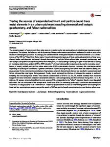
used for test computations and mapping: the Yangtze River Estuary, Hangzhou Bay, Taihu Lake, East China Sea (southern and northern parts), and Yellow Sea. The second area is the US East Coast waters area spanning the Neuse River Estuary (NRE) and Pamlico Sound (PS) (Fig. 3), which was used for the algorithm validation. The MODIS/ Aqua acquisitions were performed above the Chinese waters from 2008 – 2013, while in situ (ModMon and FerryMon spectral reflectance and chlorophyll observations59) and remote sensing (with the ENVISAT/MERIS sensor33) observations were exploited for the East US coastal waters during 2006 – 2009. 36 °N

Yellow Sea 34 °N

117%

120°2

123°E

126°E

126°E

32 °N

Yangtze River

30 °N

;Hangzhou Bay

East China Sea

Zhejiang

28' N

1N9 E

120°E

121"E

122"E

123°E

124"E

125"E

126°E

Figure 2. The study area showing six sub-areas used for the test computations (patterned rectangles). 4.

RESULTS FOR THE CHINESE NATURAL WATERS

Below we show some input and output atmospheric and water parameters for the Chinese waters observed by the MODIS/Aqua on March 24, 2012 with the spatial resolution of 1 km. A total number of pixels under investigation was n = 8435 with 813, 1174, 2248, 2483, and 1717 pixels for Yangtze River Estuary, Hangzhou Bay, Taihu Lake, East China Sea, and Yellow Sea, respectively. In turn, the East China Sea has been represented by two geographical areas lying between latitudes of 30oN and 30.5oN (southern part, 1197 pixels), and 31.5oN and 32oN (northern part, 1286 pixels), respectively. A total mean time of one scene (Figure 2) of image processing was generally ~ 20 – 30 minutes on the Intel Pentium Dual-Core E5200 Processor, 2.5 GHz. The Fig. 4 gives an example of the aerosol optical thickness (AOT) average spectra τa(λ), derived from the MODIS data using the Ångström law (Eq. 7). The numerical values of the mean AOTs are rather large, ranging from τa(550) = 0.23(±0.00) for the southern part of the East China Sea to τa(550) = 0.57(±0.04) for the Taihu Lake. Such large values may indicate the relatively high aerosol densities and large median size of aerosols fine mode45 in the area. These values


of AOT correspond to the values of the atmospheric visibilities (estimated by Eqs. (4.27) and (4.28) of Ref. [34]) varied from 27 km for the southern part of the East China Sea atmosphere to 9 km for Taihu Lake. The TOA spectral upwelling radiance Lu, TOA(λ) is shown in Fig. 5. All spectra have close spectral features: 1) a slow decrease at 410 < λ < 465 nm; 2) a sharper decrease at 465 < λ < 530 nm; 3) a slower decrease at 530 < λ < 645 nm; 4) a sharper decrease at 645 < λ < 665 nm; and 5) a slower decrease at 665 < λ < 677 nm. Of note is that a similar spectral form and numeral values were derived from the ocean-atmosphere model by Shen and Verhoef (2010)60, their Figs. 3-5.

Figure 3. The Neuse River-Pamlico Sound Estuarine System with ModMon stations and FerryMon routes. Redrawn from Sokoletsky et al. (2012)59.

0.8 Yangtze River Estuary

Taihu Lake

0.7 -

East China Sea (N)

Hangzhou Bay

East China Sea (S) ,Yellow Sea

0.6 I-

0.5 -

o

a

0.4 0.3 0.2 0.1

400

450

500

550

600

650

700

Wavelength (nm)

Figure 4. The AOTs over Chinese East Coast waters registered by the MODIS on March 24, 2012. The symbols show average values, while the vertical lines indicate standard deviation values. Two different parts of the East China Sea designated by the letter “S” (southern part) and “N”(northern part).


12 Yangtze River Estuary rn

10

E

y

Hangzhou Bay

Taihu Lake

i

East China Sea (S)

xYellow Sea

East China Sea (N)

-

C

V

t. d

$ 6

;

o

4-

,o

-

aC

¢

f

2-

O

1-

! I! i

f

-

0

400

i

i

i

i

i

450

500

550

600

650

700

Wavelength (nm)

Figure 5. The TOA radiance spectra registered by the MODIS/Aqua on March 24, 2012.

The next figures demonstrate the impact of atmospheric constituents on direct light transmittance (Fig. 6), and spectral behavior of downwelling (Fig. 7) and upwelling (Fig. 8) transmittances for the both direct and diffuse light. 1

0.95 -

I _al

0.9 0.85 -

-Rayleigh -03 +NO2 +Gases +H2O -Aerosols 0.8

400

450

500

550

600

650

700

Wavelength (nm)

Figure 6. The spectral transmittances of the direct downwelling irradiance of atmospheric constituents. Model results were obtained from the MODIS/Aqua acquisition on March 24, 2012. The mean (solid curves) and standard deviation (vertical lines) values given for the whole (n = 8435) dataset. 1

0.9 = 0.8 = 0.7 =

-Direct

-Diffuse

0.6 = 0.5 = 0.4 = 0.3 = 0.2

400

450

500

550

600

650

700

Wavelength (nm)

Figure 7. The same as Fig. 6, but for the total direct and diffuse downwelling transmittances.


1

0.9 = 0.8 =

0.7 =

-Direct -Diffuse

0.6 =

0.3 =

ii

r ---r--}--{---{-rr

04 =

r

1

1I

111

0.2 = 0.1

400

''

450

500

550

600

650

700

Wavelength (nm)

Figure 8. The same as Fig. 6, but for the total direct and diffuse upwelling transmittances. It is not surprising that aerosols and molecules contribute the greatest impact on light attenuation in the atmosphere, while a mutual impact of ozone, nitrogen dioxide, different gases and water vapor is relatively small in the visible spectral range. The aerosols cause not only the largest impact on the atmospheric transmittance over the East China natural waters, but their impact is also the most variable relative to the others constituents. It is interesting also to note the closeness of values between downwelling and upwelling transmittances that is explained by application of the reciprocity principle for transmitted light53, 54 and by the close values between solar zenith (36o±1o) and satellite zenith (35o±10o) angles at the time of scene acquisition.

Figures 9 and 10 show the spectral distribution of the TOA path (from aerosols and molecules) and sun glitter, respectively. 10 Yangtze River Estuary

N E

Taihu Lake

8

East China Sea (N)

Hangzhou Bay

East China Sea (S) Yellow Sea

6+ rs

4

L a Q

2

ca

s

0

o

0

o

400

450

500

550

600

650

700

Wavelength (nm)

Figure 9. The TOA path radiance spectra derived from the MERIS data for different Chinese natural waters on March 24, 2012.


12

1-

#

#

#

0.8 - 4 0.6 -

i

t

i

i

i

I4

:

0.4 -

Yangtze River Estuary

Hangzhou Bay

Taihu Lake

02 -

Each China Sea (S)

East China Sea (N)

xYellow Sea

0

400

450

500

600

550

650

700

Wavelength (nm)

Figure 10. The same as Fig. 9, but the TOA sun glitter spectra.

Figs. 11 and 12 demonstrate atmospherically-corrected Rrs(λ) and Lwn(λ) spectra, respectively. Both figures have the obvious spectral features related to the shift of main maximum from the green (~ 550 nm) for the coastal East China Sea waters to the red or even to the near infrared range for the other, more turbid waters. Note that this obstacle allows using the red-to-green spectral ratio as an indicator of water quality, expressed, for example, through the SSC or Kd. 0.1

0.08 -

0.06 N ce

0.04 Yangtze River Estuary

0.02 -

Hangzhou Bay

Taihu Lake

East China Sea (S)

xYellow Sea

East China Sea (N)

0

400

450

500

600

550

650

700

Wavelength (nm)

Figure 11. Remote-sensing reflectance spectra for different Chinese natural waters on March 24, 2012 derived after application of atmospheric correction.

#

Yangtze River Estuary

0

400

o

Hangzhou Bay

Taihu Lake

East China Sea (S)

East China Sea (N)

xYellow Sea

I

I

I

450

500

550

600

650

700

Wavelength (nm)

Figure 12. The same as Fig. 11, but for normalized water-leaving radiance.


It is important to note also that the spectral form of retrieved optical signals seems similar to what were observed earlier2, , even though the current numerical values may be different (generally higher) in some degree than those provided by the other in situ or remote sensing measurements and estimates. Figure 13 yields an additional confirmation for using the green-red spectral range for the water quality assessment in the Chinese natural waters by showing the contribution of the water-leaving radiance on the TOA level, Lw, TOA(λ) = Lw(λ)×Tu, dif(λ), to the total TOA signal Lu, TOA(λ). Rational here in that this contribution is much larger in the green-red range relative to the other spectral ranges, and, thus, the accuracy of retrieved Lw(λ) in that spectral range is increased. Fig. 13 shows a gradual increase from the blue to the red spectral range for all types of the waters. However, at 645 nm these contributions are significantly different for different waters, starting from 51.7±3.1% for the relatively clear southern East China Sea and ending 77.5±0.1% for the extremely turbid waters of Hangzhou Bay. We also show (in the same figure) results of numerical simulating (Monte-Carlo and successive order of scattering) for the maritime aerosol model (with RH = 80%) and three different typical waters derived from Wang et al. (2010)27. It is notable that similar results exist for the SSC-dominated waters in the ~ 400-550 nm spectral range, although our modeling results demonstrate the increasing contribution of the Lw, TOA(λ) into Lu, TOA(λ) at λ > 550 nm up to ~ 650 nm while the typical SSC-dominated waters (dash curve) have a maximum at λ ≈ 550 nm. A difference between the literature and our results is most likely due to the actual differences in the biogeochemical (and, hence, optical) situations in different natural waters. For example, Wang et al. (2010)27 found that the scattering coefficient, b(λ = 550 nm) varied between 3.1 and 3.9 m-1 in the Mauritanian coast, while our in 3, 6, 9, 11, 12, 14

90

80

Hangzhou Bay East China Sea (S) Yellow Sea - -Case 2, SSC- dominated

Yangtze River Estuary Taihu Lake East China Sea (N)

-Case 1 waters

70

---Case 2, CDOMdominated

60 50 40 30

20

`.

10 0

400

450

500

550

600

650

700

Wavelength (nm)

Figure 13. The contribution of the water-leaving radiance achieved the TOA into total signal received by the satellite’s sensor for different Chinese natural waters on March 24, 2012. The black curves illustrating three typical world waters cases are also given for comparison.

situ measurements14 performed in Yangtze River Estuary and its adjacent coastal area in May 2011 yielded b(λ = 550 nm) ranges of 53 ─ 95 and 1.9 ─ 13.0 m-1, respectively. This may indicate the larger backscattering and reflected radiance, and, therefore, the larger contribution of the water-leaving radiance to the total TOA radiance in the Chinese waters comparative to the Mauritanian coastal waters. Seasonal variations and differences in models also may contribute in discrepancies between these two results. An impact of the atmospheric correction on the Rrs(645.5)/Rrs(553.6) spectral ratio, SSC, and Kd(0o, 490 nm, 0-) for different Chinese waters observed by the MODIS/Aqua on March 24, 2012 is demonstrated in Figs. 14, 15, and 16, respectively. We use the TOA radiance reflectance spectral ratio, RL, TOA(645.5)/RL, TOA(553.6), where RL, TOA = Lu, TOA/ Ed, TOA, as a surrogate ratio for the Rrs(645.5)/Rrs(553.6) for these three figures. Thus, a mutual impact of atmospheric


path radiance and sun glitter on the TOA upwelling radiance was rejected. All figures demonstrate the great differences between the atmospherically corrected and uncorrected output quantities. 1.6 Yangtze River Estuary Hangzhou Bay Taihu Lake East China Sea (S) East China Sea (N) x Yellow Sea

1.4 1.2

-1:1 line 1.0

0.8 0.6 0.4 0.2

02

0.4

0.6

1.0

0.8

1.2

1.4

16

RLTOa(645.5)/RL,TOn(553.6)

Figure 14. A demonstration of the impact of the AC on the Rrs(645.5)/Rrs(553.6) spectral ratio in accordance with our atmospheric correction model for different Chinese waters observed by the MODIS/Aqua on March 24, 2012. 1280

640 320 -

Yangtze River Estuary Hangzhou Bay Taihu Lake East China Sea (S)

East China Sea (N)

160

1 Yellow Sea

80 40 20 10 5

10

20

40

80

160

SSC (g m-3) - without atmospheric correction

Figure 15. The same as Fig. 14, but for SSC. 62.5 12.5 E

R 2.5

E

Yangtze River Estuary Hangzhou Bay Taihu Lake East China Sea (S) East China Sea (N) Yellow Sea

0.5

C 0.1

0.02 0.02

0.1

0.5

2.5

12.5

Ká(490) (m-1) - without atmospheric correction

Figure 16. The same as Fig. 14, but for Kd(0o, 490 nm, 0-).


Calculations show that at RL, TOA(645.5)/RL, TOA(553.6) ≈ 0.6, outputs are the same with and without AC. However, at RL, TOA(645.5)/RL, TOA(553.6) < 0.6 or RL, TOA(645.5)/RL, TOA(553.6) > 0.6, the AC procedure causes a decrease or increase in outputs, respectively. Figure 17 shows examples of the produced color (false) images for the SSC (left side) and Kd(0o, 490, 0-) (right side) values in the East China coastal area. Kd(0 °,490nm) with atm.cor.,UTC 5:20,May 16,2008

SSC with atm.cor.,UTC 5:20,May 16,2008 36°N

36°N

34 °N

34 °N

32°N

32°N

30 °N

30 °N

28118°E

120 °E

m

io

121 °E

40

122 °E

80

123°E Lon ieo

124 °E

320

640

125 °E

126 °E

34 °N

32°N

30 °N

28119°E

2560

1280

0 n5

SSC with atm.cor.,UTC 5:35,May 10,2009 36°N

120 °E

121 °E

0z

0f

0s

122 °E

123°E Lon

8

1

SSC(mg/L)

124 °E

125 °E

126 °E

28119°E

120 °E

121 °E

124 °E

125 °E

640

1280

126 °E

Lon 16

32

64

128

256

20

10

40

80

Kd(1 /m)

320

160

2560

SSC(mg/L)

Kd(0 °,490nm) with atm.cor.,UTC 5:10,May 24,2010

SSC with atm.cor.,UTC 5:10,May 24,2010 Kd(0 °,490nm) with atm.cor.,UTC 5:35,May 10,2009

123°E

122 °E

36°N

36°N

34 °N 34 °N

32°N

32°N

28118°E

28119°E

0 a5

30 °N

30 °N

30 °N

120°E

0 .i

0z

121°E

05

122°E 123°E Lon

8

1

Kd(1/m)

124°E

16

32

125°E

64

128

126°E

zss

120 °E

121 °E

122 °E

123 °E

124 °E

125 °E

640

1280

126 °E

26119°E

120°E

121°E

122°E 123°E Lon

Lon 10

20

40

80

160

320

2560

0 a5

SSC(mg/L)


0 .i

0z

05

8

1

Kd(1/m)

124°E

16

32

125°E

64

128

126°E

zss

SSC with atm.cor.,UTC 5:15,May 18,2011

SSC with atm.cor.,UTC 5:25,Mar 24,2012


36 N

36°N

36 N

34 °N

34 °N

34©N

32 °N

32°N

32©N

30 °N

30 °N

30 °N

2119 °E

120 °E

121 °E

122 °E

.0

0

123 °E

124 °E

Lon

125 °E

126 °E

28119°E

121 °E

122 °E

123 °E

124 °E

125 °E

126 °E

28119 °E

Lon 640

80 SSC(m9/L)m

120 °E

121 °E

122 °E

20

40

30

Kd(1/m)

Kd(0 °,490nm) with atm.cor.,UTC 5:25,Mar 24,2012

123 °E

124 °E

126 °E

sa

imo

126 °E

Lon

2560

1280

36°N

SSC(mg /L)320

SSC with atm.cor.,UTC 5:30,Apr 12,2013 Kd(0 °,490nm) with atm.cor.,UTC 5:30,Apr 12,2013

36°N 36°N

34 °N

34 °N

32°N

32°N

30 °N

30 °N

28119°E

120 °E

34 °N

120 °E

123°E Lon

121 °E

122 °E

124 °E

125 °E

126 °E

32°N

30 °N

28118°E

10

120 °E

20

123°E Lon

121 °E

40

Kd(1/m)

122 °E

80

160

320

124 °E

640

125 °E

1280

126 °E

28119°E

2560

0 a5

120 °E

0z

0 .i

123°E Lon

121 °E

05

122 °E

8

1

16

32

125 °E

64

128

126 °E

zss

Kd(1/m)

SSC(mg/L)

SSC with atm.cor.,UTC 5:35,Apr 26,2013

124 °E

Kd(0 °,490nm) with atm.cor.,UTC 5:35,Apr 26,2013

36°N

36°N

SSC with atm.cor.,UTC 5:40,May 13,2013 36 °N

34 °N

34 °N 34 °N

32°N

32°N

30 °N

30 °N

28118°E

10

120 °E

20

121 °E

40

123°E Lon

122 °E

80

160

SSC(mg/L)

320

124 °E

640

125 °E

1280

126 °E

28119°E

32 °N

30 °N

120 °E

121 °E

123°E Lon

122 °E

124 °E

125 °E

126 °E

281%°E

121 °E

123 °E

122 °E

124 °E

125 °E

640

12E0

126 °E

Lon 10

2560

120 °E

Kd(1/m)


20

40

80

160

SSC(mglL)

320

2560


Kd(0°,490)with atm.cor.,UTC 4:50,Sep 15,2013

36°t

36 N

34°t

34°N

32°t

32°N

30 °N

30 °N

28116E

0 a5

120°E

0 .i

0z

121°E

05

122°E 123°E Lon

8

1

Kd(1/m)

124°E

16

32

125°E

64

128

126°E

zss

30°N

28119°E

io

120°E

m

121°E

40

122°E 123°E Lon 80

ieo

320

124°E

125°E

126°E

28119 °E

120 °E

121 °E

122 °E

123 °E

124 °E

125 °E

126 °E

L0 n 640

1280

2560

SSC(mg/L)

Kd(ilm)

Figure 17. Examples of the SSC (left side) and Kd(0o, 490, 0-) (right side) mapping of the East China coastal waters by simplified analytical algorithm developed in the study. Land, clouds and suspicious pixels are colored white, as explained in detail in the text. 5.

VALIDATION OF THE ATMOSPHERIC CORRECTION AND THE WATER QUALITY ALGORITHMS

An initial validation of the represented atmospheric correction algorithm may be made by comparison of our Rrs(λ) and Lwn(λ) values with the literature data. As mentioned above, the literature data2, 3, 6, 9, 11, 12, 14 confirm a correctness of their spectral forms for the Chinese natural waters. Also, several publications2-6, 9 give in situ and remote sensing SSC values that are close to our range (from almost zero to 2500 g m-3 and even higher) found for the East China coastal waters. Our SSC and Kd(490) maps also confirm that the Hangzhou Bay, Yangtze River Estuary and Subei Bank of the Yellow Sea are extremely turbid waters, although a degree of their turbidity is seasonally and spatially variable1-6, 10, 12. However, the values of Kd(490) < 250 m-1 found from the current study are significantly greater than those were found previously (< 5 m-1 ; < 10 m-1 , and < 59 m-1 according to Refs. 10-12, 13, and 14, respectively). Thus, an additional validation of our AC algorithm for the East China coastal waters is necessary. Nevertheless, Fig. 18 gives the indirect validation of the current AC algorithm for the US East Coast waters. Two series of in situ observations were undertaken in 2006 ─ 2009 in support of remote sensing efforts: ModMon (regular field and laboratory observations) and FerryMon (permanent observations from ferries)33, 59. The Rrs(709)/Rrs(665) spectral ratio has been used as an index of the chlorophyll a concentration. The three-year dynamics of this ratio was estimated from the both in situ measurements and MERIS observations. Fig. 18 provides an example of the Rrs(709)/Rrs(665) spectral ratio data for the central station (34o57.165'N, 76 o48.831'E) of the Neuse River, NC, US. The ±3-hour time window and distance of less than 300 m between satellite overpass and this station were selected for this figure. The figure clearly demonstrates the closeness between the ModMon, FerryMon, and results of the current AC algorithm, especially during the strong phytoplankton bloom (January ─ March 2007). The results of the previously published AC algorithm33 (black crosses) and results obtained without any AC (yellow triangles) are also shown for comparison.


ln situ (ModMon) In situ (FerryMon) RS (without AC) RS (with AC: current version) x RS (with AC: "Remote Sensing ", 2011)

x

l Jan -06

Jul -06 Dec -06 Jul -07 Dec -07 Jun -08 Dec -08 Jun -09 Dec -09 Month of the Year

Figure 18. Much-up values of Rrs(709)/Rrs(665) spectral ratio measured during ModMon (a blue curve with symbols) and FerryMon (green circles) in situ observations, as well as Rrs(709)/Rrs(665) values predicted from the MODIS data as follows: without AC (yellow triangles), by the current AC algorithm (purple squares), and by the previously published AC algorithm33 (black crosses) are shown for the central station of the Neuse River, NC, US (2006-2009). The ±3-hour time window and distance less than 300 m between satellite overpass and in situ measurements were selected for this figure. 6. CONCLUSIONS A completely analytical atmospheric correction algorithm has been developed as a continuation of attempts24, 29-33 to create a simple AC algorithm for any types of natural waters, without any preliminary assumptions about spectral behavior and numerical values of the water-leaving radiance. The new AC algorithm is similar to that which was developed earlier for the eastern US waters33, although it uses a much more meticulous analysis. The SSC and Kd(490) computations and mapping of the East China coastal waters on the base of this AC algorithm are also presented and analyzed. An initial validation of suggested AC and water quality algorithm for Chinese and American inland, estuarine, and coastal waters is provided.

ACKNOWLEDGMENTS We thank Dr. Chris Gueymard from the Solar Consulting Services for the valuable discussion on the optical atmospheric model. The research leading to these results has received funding from the National Science Foundation of China (grant numbers 41371346 and 41271375) and the Doctoral Fund of Ministry of Education of China (grant number 20120076110009). 7.

REFERENCES

[1] Salama, M. S. and Shen, F., “Simultaneous atmospheric correction and quantification of suspended particulate matters from orbital and geostationary earth observation sensors,” Est. Coast. Shelf Sc. 86, 499-511 (2010). [2] Shen, F., Verhoef, W., Zhou, Y., Salama, M. S. and Liu, X., “Satellite estimates of wide-range suspended sediment concentrations in Changjiang (Yangtze) estuary using MERIS data,” Est. Coasts 33, 1420-1429 (2010). [3] Zhang, M., Tang, J., Dong, Q., Song, Q. and Ding J., “Retrieval of total suspended concentration in the Yellow and East China Seas from MODIS imagery,” Rem. Sens. Envir. 114, 392-403 (2010). [4] Shen, F., Zhou, Y., Li, J., He, Q. and Verhoef, W., “Remotely sensed variability of the suspended sediment concentration and its response to decreased river discharge in the Yangtze estuary and adjacent coast,” Cont. Shelf Res. 69, 52-61 (2013). [5] Shen, F., Zhou, Y., Peng, X. and Chen, Y. “Satellite multi-sensor mapping of suspended particulate matter in turbid estuarine and coastal ocean, China,” Int. J. Rem. Sens. 35(11-12), 4173-4192 (2014).


[6] He, X., Bai, Y., Pan, D., Tang, J. and Wang, D., “Atmospheric correction of satellite ocean color imagery using the ultraviolet wavelength for highly turbid waters,” Opt. Express 20(18), 20754-20770 (2012). [7] Wang, J. J., Lu, X. X. and Zhou, Y., “Retrieval of suspended sediment concentrations in the turbid waters of the Upper Yangtze River using Landsat ETM+,” Chinese Sc. Bul. 52 (Supp. II), 273-280 (2007). [8] Wang, J. J. and Lu, X. X., “Estimation of suspended sediment concentrations using Terra MODIS: An example from the Lower Yangtze River, China,” Sc. Total Envir. 408, 1131-1138 (2010). [9] Shen, F., Salama, M. S., Zhou, Y., Li, J., Su, Zh. and Kuang, D., “Remote-sensing reflectance characteristics of highly turbid estuarine waters – a comparative experiment of the Yangtze River and the Yellow River,” Int. J. Rem. Sens. 31(10), 2639-2654 (2010). [10] Shi, W. and Wang, M., "Satellite observations of the seasonal sediment plume in central East China Sea," J. Mar. Syst.82, 280-285 (2010). [11] Wang, M., Shi, W. and Tang, J., “Water property monitoring and assessment for China’s inland Lake Taihu from MODIS-Aqua measurements,” Rem. Sens. Envir. 115, 841-854 (2011). [12] Wang, M., Shi, W. and Jiang, L., “Atmospheric correction using near-infrared bands for satellite ocean color data processing in the turbid western Pacific region,” Opt. Express 20(2), 741-753 (2012). [13] Qiu, Zh., Wu, T., and Su, Y., “Retrieval of diffuse attenuation coefficient in the China seas from surface reflectance,” Opt. Express 21(13), 15287-15297 (2013). [14] Sokoletsky, L. G. and Shen, F., “Optical closure for remote-sensing reflectance based on accurate radiative transfer approximations: the case of the Changjiang (Yangtze) River Estuary and its adjacent coastal area, China,” Int. J. Rem. Sens. 35(11-12), 4193-4224 (2014). [15] Sokoletsky, L. G., Budak, V. P., Shen, F. and Kokhanovsky, A. A., “Comparative analysis of radiative transfer approaches for calculation of plane transmittance and diffuse attenuation coefficient of plane-parallel light scattering layers,” Appl. Opt. 53(3), 459-468 (2014). [16] Budak, V. P., Klyuykov, D. A. and Korkin, S. V., “Complete matrix solution of radiative transfer equation for PILE of horizontally homogeneous slabs,” J. Quant.Spectrosc. Radiat. Trans. 112, 1141-1148 (2011). [17] Gordon, H.R., Brown O. B. and Jacobs, M. M., “Computed relationships between the inherent and apparent optical properties of a flat homogeneous ocean,” Appl. Opt. 14(2), 417-427 (1975). [18] Gordon, H.G.,“Can the Lambert-Beer law be applied to the diffuse attenuation coefficient of ocean water?,” Limnol. Oceanogr. 34(8), 1389-1409 (1989). [19] Kirk, J. T. O., “Volume scattering function, average cosines, and the underwater light field,” Limnol. Oceanogr. 36(3), 455-467 (1991). [20] Ben-David, A., “Multiple-scattering effects on differential absorption for the transmission of a plane-parallel beam in a homogeneous medium,” Appl. Opt. 36 (6), 1386-1398 (1997). [21] Lee, Z. P., Du, K. P., and Arnone, R., “A model for the diffuse attenuation coefficient of downwelling irradiance,” J. Geophys. Res. 110(C2), C02016 (2005). [22] Gordon, H. R. and Clark, D. K., “Clear water radiances for atmospheric correction of coastal zone color scanner imagery,” Appl. Opt. 20(24), 4175-4180 (1981). [23] Gordon, H. R. and Wang, M., “Retrieval of water-leaving radiance and aerosol optical thickness over the oceans with SeaWiFS: a preliminary algorithm,” Appl. Opt. 33(3), 443-452 (1994). [24] Ruddick, K. G., Ovidio, F. and Rijkeboer, M., Atmospheric correction of SeaWiFS imagery for turbid coastal and inland waters,” Appl. Opt. 39(6), 897-912 (2000). [25] Wang, M., “Remote sensing of the ocean contributions from ultraviolet to near-infrared using the shortwave infrared bands: simulations,” Appl. Opt. 46(9), 1535-1547 (2007). [26] He, X., Bai, Y., Pan, D., Tang, J. and Wang, D., “Atmospheric correction of satellite ocean color imagery using the ultraviolet wavelength for highly turbid waters,” Opt. Express 20(18), 20754-20770 (2012). [27] Wang, M., Gordon, H. R. and Morel, A., “Atmospheric Correction for Remotely-Sensed Ocean-Colour Products,” Ch. 3 in Reports of the International Ocean-Colour Coordinating Group (IOCCG), No. 10. Wang, M. (ed.), Dartmouth, Canada, 15-22 (2010). [28] Kotchenova, S. Y., Vermote, E. F., Levy, R. and Lyapustin, A., “Radiative transfer codes for atmospheric correction and aerosol retrieval: intercomparison study,” App. Opt. 47(13), 2215–2226 (2008). [29] Rahman, H. and Dedieu, G., "SMAC: a simplified method for the atmospheric correction of satellite measurements in the solar spectrum," Int. J. Rem. Sens. 15(1), 123-143 (1994). [30] Sturm, B. and Zibordi, G., “SeaWiFS atmospheric correction by an approximate model and vicarious calibration,” Int. J. Rem. Sens. 23(3), 489-501 (2002).


[31] Guanter, L., “New algorithms for atmospheric correction and retrieval of biophysical parameters in Earth Observation. Application to ENVISAT/MERIS data,” Ph.D. Diss. University of Valencia, Valencia, Spain (2006). [32] Gong, S., Huang, J., Li, Y. and Wang, H., “Comparison of atmospheric correction algorithms for TM image in inland water,” Int. J. Rem. Sens. 29(8), 2199-2210 (2008). [33] Sokoletsky, L. G., Lunetta, R. S., Wetz, M. S. and Paerl, H. W., “MERIS retrieval of water quality components in the turbid Albemarle-Pamlico Sound Estuary, USA,” Remote Sensing 3(4), 684-707 (2011). [34] Gueymard, C., “SMARTS2, a simple model of the atmospheric radiative transfer of sunshine: Algorithms and performance assessment,” Report FSEC-PF-270-95, Florida Solar Energy Center, Cocoa, FL (1995). [35] Gueymard, C. A., “Parameterized transmittance model for direct beam and circumsolar spectral irradiance,” Solar Energy 71(5), 325-346 (2001). [36] Gueymard, C. A., “Direct solar transmittance and irradiance predictions with broadband models. Part I: detailed theoretical performance assessment,” Solar Energy 74, 355-379 (2003). [37] Gueymard, C. A., “REST2: High-performance solar radiation model for cloudless-sky irradiance, illuminance, and photosynthetically active radiation – Validation with a benchmark dataset,” Solar Energy 82, 272-285 (2008). [38] Gordon, H. R. and Castaño, D. J., “Coastal Zone Color Scanner atmospheric correction algorithm: multiple scattering effects,” Appl. Opt. 26(11), 2111-2122 (1988). [39] Cox C. and Munk, W., “Measurement of the roughness of the sea surface from photographs of the sun’s glitter,” J. Opt. Soc. Amer. 44(11), 838-850 (1954). [40] Exell, R. H. B., “A mathematical model for solar radiation in South-East Asia (Thailand),” Solar Energy 26(2), 161–168 (1981). [41] Duffie, J.A. and Beckman, W.A., “Solar Engineering of Thermal Processes,” Wiley: New York, NY, USA (1991). [42] Rigollier, C., Bauer, O. and Wald, L., “On the clear sky model of the 4th European Solar Radiation Atlas with respect to the Heliosat method,” Solar Energy 68(1), 33-48 (2000). [43] Spenser, J. W., “Fourier series representation of the position of the sun,” Search 2(5), 172 (1971). [44] Ångström, A, “Techniques of determining the turbidity of the atmosphere,” Tellus, 13, 214-223 (1961). [45] Dubovik, O., Holben, B., Eck, T.F., Smirnov, A., Kaufman, Y.J., King, M.D., Tanre, D., and Slutsker, I., “Variability of absorption and optical properties of key aerosol types observed in worldwide locations,” J. Atm. Sci. 59, 590-608 (2002). [46] Gueymard, C. A. and Thevenard, D., “Monthly average clear-sky broadband irradiance database for worldwide solar heat gain and building cooling load calculations,” Solar Energy 83, 1998-2018 (2009). [47] Haltrin, V. I., “Two-term Henyey-Greenstein light scattering phase function for seawater,” Proc. IGARSS’99, Hamburg, Germany, ed. Tammy I. Stein (1999). [48] Aranuvachapun, S., “Variation of atmospheric optical depth for remote sensing radiance calculations,” Rem. Sens. Envir. 13, 131-147 (1983). [49] Sokoletsky, L. G., Kokhanovsky, A. A. and Shen, F., “Comparative analysis of radiative transfer approaches for calculation of diffuse reflectance of plane-parallel light scattering layers,” Appl. Opt. 52(35), 8471-8483 (2013). [50] Lu, Z., “Optical absorption of pure water in the blue and ultraviolet,” Ph.D. Diss., Texas A & M University, Texas, USA (2006). [51] Pope, R. M. and Fry, E. S., “Absorption spectrum (380-700 nm) of pure water. II. Integrating cavity measurements,” Appl. Opt. 36(33), 8710-8723 (1997). [52] Zhang, X., Hi, L. and He, M.-X., “Scattering by pure seawater: Effect of salinity,” Optics Express 17(7), 56985710 (2009). [53] Sekera, Z., “Reciprocity relations for diffuse reflection and transmission of radiative transfer in the planetary atmosphere,” Astrophys. J. 162, 3-16 (1970). [54] Yang, H. and Gordon, H. R., “Remote sensing of ocean color: assessment of water-leaving radiance bidirectional effects on atmospheric diffuse transmittance,” Appl. Opt. 36(30), 7887-7897 (1997). [55] Gordon, H. R. and Voss, K. J., “MODIS Normalized Water-leaving Radiance Algorithm Theoretical Basis Document (MODIS 18), Version 5,” Univ. Miami, Coral Gables, FL, US (2004). [56] Gao, Bo-Cai, Yang, P., Han, W., Li, R.-R. and Wiscombe, W. J., “An algorithm using visible and 1.38- m channels to retrieve cirrus cloud reflectances from aircraft and satellite data,” IEEE Trans. Geosci. Remote Sensing 40(8), 1659-1668 (2002). [57] Wang, M. and Shi, W., “Cloud masking for ocean color data processing in the coastal regions,” IEEE Trans. Geosci. Remote Sensing 44(11), 3196-3205 (2006).


[58] Kahru, M., “Exercises using MODIS 250-m bands by Mati Kahru (2004-2008),” http://www.wimsoft.com/Course/2_Level_1B/Exercises_modis_250m.pdf. [59] Sokoletsky, L. G., Lunetta, R. S., Wetz, M. S. and Paerl, H. W., “Assessment of the water quality components in turbid estuarine waters based on radiative transfer approximations,” Israel J. Plant Sci. 60, 209-229 (2012). [60] Shen, F. and Verhoef, W., “Suppression of local haze variations in MERIS images over turbid coastal waters for retrieval of suspended sediment concentration,” Optics Express 18(12), 12653-12662 (2010).
