Modular FPGA-Based Digital Ultrasound Beamforming Mawia A. Hassan, Abou-Bakr M. Youssef, Yasser M. Kadah Systems & Biomedical Engineering Department Cairo University Giza, Egypt
[email protected] Abstract— The evaluation of ultrasound system is measured by the development in analog and digital electronics. A modular field programmable gate array (FPGA)-based digital ultrasound beamforming is presented. The digital beamforming is implemented in Virtex-5 FPGA. The objective of this work is to develop a modular low-cost PC-based digital ultrasound imaging system that has almost all of its processing steps done on the PC side. The system consists of: two 8 channels block and reconstructed line block. The 8 channel block consist of: memory block to save the samples data after converted to fixed point type, delay block implemented by addressable shift register - the delay process is based on sampled delay focusing (SDF) - and M-code block applied the summation of each RF channel samples. The reconstructed block consists of pipelined adder to apply the summation of the two 8 channels blocks. The power consumption and device utilization was acceptable. Also it is possible to build 16-,32-,64-,and 128-channel beamformer. The hardware architecture of the design provided flexibility for beamforming. Keywords-ultrasound; digital beamforming; FPGA I.
INTRODUCTION
Different articles introduced the issues involved in digital beamformer design including the description of its main components. Embedded digital beamforming was initially done using Application-Specific Integrated Circuits (ASICs) [6]. Many approaches also described the digital signal processing algorithms that can be used in digital beamforming signal demodulation [7][8][9]. Real-time digital ultrasound imaging is described in [10]. A compact medical ultrasound beamformer architecture that uses oversampled 1-bit analog-to-digital converters (ADC) is presented in [11]. However, the development in ADC and FPGA technologies, make it is possible to use fast analog acquisition like serial low voltage differential signaling (LVDS) interface protocol, which makes the output from an ADC to come as a serial bit stream with drivers on both the ADC and the FPGA to recover the parallel data. This reduces the need for designing the sigma-delta sampling and the signal recovery filters for the oversampled 1-bit data stream while maintaining an optimal.
With the growing availability of high-end integrated analog front-end circuits, distinction between different digital ultrasound imaging systems is determined almost exclusively by their software component. Our previous work concerned on description the digital ultrasound imaging system [1] and the processing steps which done on the PC side [2].
In this paper, a modular FPGA-based digital ultrasound beamforming is presented. The digital beamforming is implemented in Virtex-5 FPGA (Xilinx, Inc.). This paper is extending of our previous work [1] [2].
A commonly used approach to image acquisition in ultrasound system is digital beamforming. Digital beamforming, as applied to the medical ultrasound, is defined as phase alignment and summation [3] of signals that are generated from a common source, by received at different times by a multi-elements ultrasound transducer [4].
A. Linear Array Reconstruction Selected of a group of elements (aperture) whose location is defines the phase center of the beam [12]. Electronic focusing was applied on receive for each aperture. Received at the aperture elements are delayed by focusing delays and summed to form scan line in the image. After that one elements shift is applied to the aperture and the process was repeated till the end of the array elements at the outer side processing all image scan lines (Fig. 1 where aperture equal 16 elements). The number of lines is equal to the total number of elements minus the number of the aperture elements plus one.
The commonly use arrays are linear, curved, or phase array. The important distinctions arise from the method of beam steering use with these arrays. For linear and curve linear, the steering is accomplished by selection of a group of elements whose location defines the phase center of the beam. In contrast to linear and curve linear array, phase array transducer required that the beamformer steers the beam with switched set of array elements [5]. These requirements mention important differences in complexity over the linear and curved array. Beamformer has two functions: directivity to the transducer (enhancing its gain) and defines a focal point within the body, from which location of the returning echo is derived.
978-1-4244-7000-6/11/$26.00 ©2011 IEEE
II.
METHODOLOGIES
Figure 1. Linear array elements
C. Delay Equation Fig. 2 shows the geometry which is used to determine the channel and depth-dependent delay of a focused transducer array. After a wave-front is transmit into the medium an echo wave propagates back from the focal points (P) to the transducer. Which c denoting the speed of sound in the medium, the distance from P to the origin is given by [13]:
ti = Figure 2. Geometry of a focused transducer array
B. Linear Phase Array Reconstruction In contrast the linear array, phase array transducer required that the beamformer steered the beam with an unswitched set of array elements [12]. This reconstruction technique divides the field of view (FOV) into different point targets (raster points), P(i,j). Each point represented as an image pixel, which is separated laterally and axially by small distances. Each target is considered as a point source that transmits signals to the aperture elements. The beamforming timing is then calculated for each point based on the distance R between the point and the receiving element, and the velocity of ultrasonic beam in the media. Then the samples corresponding to the focal point are synchronized and added to complete the beamforming as the following: N
PD (i, j ) = ∑ X n (K i , j ),
(1)
n =1
where PD (i,j) is the signal value at the point whose its coordinates are (i,j), and Xn (Ki,j) is the sample corresponding to the target point in the signal Xn received by the element number n. The sample number Ki,j which is equivalent to the time delay is calculated using the equation below:
K i, j =
Rn (i, j ) . T ×c
(2)
Here Rn (i, j) is the distance from the center of the element to the point target, c is the acoustic velocity via the media, and T is the sampling period of the signal data.
Figure 3. Architecture implementation of the modular FPGA-Based digital ultrasound receive beamformer blocks
1 ( xi − x f ) 2 + ( yi − y f ) 2 . c
(3)
Where (xf ,yf) is the position of the focal point, (xi ,yi) is the center for the physical element number i, and c is the speed of sound. A point is selected on the whole aperture (AP) as a reference (xc ,yc) for the imaging process. The propagation time (tc) for this was calculated as in equation (3), but the distance here from P to the reference (xc ,yc). The delay to use on each element (ti) of the array is then [13][14]:
Δti = tc − ti
(4)
D. Implementation Steps A typical architecture implementation of the modular FPGA-based digital ultrasound receive beamformer is shown in Fig.3. The system consist of: Two 8 channels block and reconstructed line block. The beamfomer is done by using Xilinx system generator (Xilinx, Inc.) and MATLAB simulink (MathWorks, Inc.). The digital beamforming is implemented in Virtex-5 FPGA. The RF data saved in MATLAB workspace and used Xilinx block to read the one dimension RF data from workspace. The implementation steps are: 1) The RF data saved in MATLAB workspace and used Xilinx block to read the one dimension RF data from workspace. 2) The RF data then convert the double precision data type to fixed point numeric precision for hardware efficiency. 3) Verified the fixed-point Model by compared the fixedpoint results to the floating-point results and determine if the quantization error is acceptable. 4) After verified the model, each channel data saved in memory block. The memory word size is determined by the bit width of the channel data. The memory controlled by wire enable port with 1 indicates that the value of the channel data should be written to the memory address pointed to by step-up counter. 5) The delay process is based on sampled delay focusing (SDF). The delays calculated using the same method in section C Then the delays converted to number of samples by divided the delays by the sampling time. SDF consist of addressable shift register (ASR) to delay the sampled signals, and M-code Xilinx block that contain the calculated delays. The samples are delayed by the value in the address input of the ASR. 6) After delaying each RF channel samples, the summation is applied using M-code block to summate the 8 channel signals.
7) The summation of the two 8 channels is connected to adder to reconstructed the final focus line. 8) Modify the bit of the signal to 16 bit using bit modifier block. 9) In order to obtain performance and logic utilization figures for the suggestion architecture, it was implemented in the hardware description language (VHDL) and synthesized with Virtex-5 FPGA. III.
Figure 6. 100 samples of channel 8 and 9 data after synchronization
RESULTS
A. The Ultrasound Data We used correct real data obtained from the Biomedical Ultrasound Laboratory, University of Michigan [15]; the data set that was used to generate the results here is under "Acusonl7". The parameters for this data set are as follows: the number of channels was 128 channels, and the ADC sampling rate was 13.8889 MSPS. Linear shape transducer was used to acquire the data with center frequency of 3.5 MHz, and element spacing of 0.22mm. Each ultrasonic A-scan was saved in a record consisted of 2048 RF samples per line each represented in 2 bytes, and the signal averages was 8. The speed of the ultrasound in the phantom was 1480 m/sec. The data were acquired for phantom within 6 pins at different positions. The data was used to build the N-channel beamformer on receive as discussed in methodologies. B. Verify the Fixed-point Model Fig. 4 shown double precision RF data type read from MATLAB work space compared to fixed point RF data type for hardware efficiency. We verified the fixed-point Model by subtract the fixed-point RF signal from the floating-point RF signal and the result equal zero. This means zero quantization error. C. Delays Table I shown the calculated delays as in section C and converted delays to number of samples and rounding these values. Fig. 5 and Fig.6 illustrated 100 samples of channels 8 and 9 data respectively before and after synchronization. They had same arrival times in Fig.6 compared to Fig.5.
Figure 4. Comparison between Floating and Fixed point RF signal
Figure 5. 100 samples of channel 8 and 9 data before synchronization
Figure 7. Comparison between simulated and implemented the first line in image reconstruction
D. The Reconstructed Line Fig. 7 shown the comparison between implemented the first line in image reconstruction and the simulated one [2].As can be shown the implementation result was the same as the simulation result. E. Device Utilization Table II shown the device utilization summary for the whole implementation, the used devices, available in the port, and the utilization in percentage using Virtex-5 FPGA. F. Image Reconstruction Fig. 8 showed the linear phase reconstruction to reconstructed image of six pins phantom from the data set. Image reconstructed using raster point technique. Fig. 9 described the point spread function (PSF) for the first pin as indicated by arrow in Fig. 8. IV.
DISCUSSIONS
From the results the fixed-point Model is the same as the floating point mode and this is an important for hardware efficiency (Fig. 4 and Fig.5). Moreover, the delays applied as SDF gave a synchronous in the time of arrival (Fig. 6). Further, the comparison between implemented the first line in image reconstruction and the simulated introduce a good results (Fig. 7). Furthermore, the reconstructed image of the six pin gave a good FOV and lateral resolution (Fig. 8). In addition, the PSF presented a quantitative measure of the beamforming qualityTABLE I. Channel # Channel # 1 and 16 Channel # 2 and 15 Channel # 3 and 14 Channel # 4 and 13 Channel # 5 and 12 Channel # 6 and 11 Channel # 7 and 10 Channel # 8 and 9
THE SDF VALUES
Delay Value (ns) 0 4.1942 7.7895 10.7860 13.1830 14.9810 16.180 16.7790
Number of Samples 0 0.0583 0.1082 0.1498 0.1831 0.2081 0.2247 0.2330
Rounding Value 0 1 1 1 1 1 1 1
TABLE II. Slice Logic Utilization Number of Slice Registers Number used as Flip Flops Number of Slice LUTs Number used as logic Number using O6 output only Number using O5 output only Number using O5 and O6 Number used as Memory
DEVICE UTILIZATION SUMMARY
Used 22 22 500 242 216 18 8 256
Available 207,360 207,360 207,360 54,720
Utilization 1% 1% 1% 1%
Number used as Shift Register
256
-
-
Number using O6 output only Number used as exclusive route-thru
256 2
-
-
Slice Logic Utilization Number using O6 output only Number using O5 output only Number of occupied Slices Number of LUT Flip Flop pairs used Number with an unused Flip Flop Number with an unused LUT Number of fully used LUT-FF pairs Number of unique control sets Number of slice register sites lost to control set restrictions Number of bonded IOBs Average Fanout of Non-Clock Nets
Number of route-thrus
26
-
-
-
and hence determines the ultrasound system power (Fig. 9).In addition to, the power consumption and device utilization was acceptable. V.
CONCLUTIONS
In this paper, a modular FPGA-based digital ultrasound beamforming is presented. The digital beamforming is implemented in Virtex-5 FPGA. The power consumption and device utilization was acceptable. It is possible for the system to accept anther devices for further processing. Also it is possible to build 16-, 32-, 64-, and 128-channel beamformer. The hardware architecture of the design provided flexibility for beamforming. The 16-channel beamformer is implemented in one FPGA chip, which reduces hardware complexity. The system has the potential to lower the cost and speed up the development, thus offering new opportunities for more costeffective systems.
[1]
[2]
[3]
[4]
[5] [6]
[8]
[9]
[10]
[11]
[12] [13]
[14] [15]
Figure 9. PSF of the first pin
Available 51,840 500 500 500 -
Utilization 1% 95% 0% 4% -
2
207,360
1%
1,009 1.68
1,200 -
84% -
-
-
-
REFERENCES
[7]
Figure 8. Reconstructed image of six pins phantom
Used 20 6 200 500 478 0 22 2
A. M. Hendy ,M. A. Hassan, R. Eldeeb, D. Kholy, A. Youssef and Y. M. Kadah, “PC-Based Modular Digital ultrasound Imaging system,” in Proc. IEEE Ultrason. Symp., Rome, Italy, September 2009, pp.13301333. M. A. Hassan, A. S. Mohamed, A. M. Youssef, and Y. M. Kadah, “Signal Processing Methodologies for Digital Beamforming and Image Reconstruction in Ultrasound Imaging,” in Proc. 27th National Radio Science Conference, Menouf, Egypt, March 2010,p. K10.1-K10.12. R.A. Mucci, “A Comparison of Efficient Beamforming Algorithms,” IEEE Trans. Acoustics, Speech, And Signal Proc., vol. 32. 1984, pp. 548-558. R. Reeder, C. Petersen, “The AD9271-A Revolutionary Solution for Portable Ultrasound,” Analog Dialogue 41-07,Analog Devices, July 2007. K. E. Thomenius, “Evaluation of Ultrasound Beamformers,” in Proc. IEEE Ultrason. Symp., 1996, pp.1615-1621. B.D. Steinberg, “Digital beamforming in ultrasound,” IEEE Transactions on Ultrasonics, Ferroelectrics and Frequency Control, vol. 39, no. 6, 1992, pp.716-721. C. Fritsch, M. Parrilla, T. Sanchez, O. Martinez, “Beamforming with a reduced sampling rate,” Ultrasonics, vol. 40, 2002, pp. 599–604. S. R. Freeman, M. K. Quick, M. A. Morin, R. C. Anderson, C. S. Desilets, T. E. Linnenbrink, and M. O’Donnell, “Delta sigma oversampled ultrasound beamformer with dynamic delays,” IEEE Trans. Ultrason., Ferroelect., Freq. Contr., vol. 46, 1999, pp. 320–332. M. Kozak and M. Karaman, “Digital phased array beamforming using single-bit delta-sigma conversion with non-uniform oversampling,” IEEE Trans. Ultrason., Ferroelect., Freq. Contr., vol. 48, 2001, pp. 922–931. C. Basoglu, R. Managuli, G. York, and Y. Kim, “Computing requirements of modern medical diagnostic ultrasound machines,” Parallel Computing, vol. 24, 1998, pp. 1407-1431. B.G. Tomov and J.A. Jensen, “Compact FPGA-Based Beamformer Using Oversampled 1-bit A/D Converters,” IEEE Transactions on Ultrasonics, Ferroelectrics and Frequency Control, vol. 52, no. 5, May 2005, pp. 870-880. D. A .Christensen, Ultrasonic Bioinstrumentation, Jonh Wiley & Sons, New York, 1988. J. A. Jensen, “Ultrasound imaging and its Modeling”, Department of Information Technology, Technical University of Denmark, Denmark, 2000. Szabo, T. L., Diagnostic Ultrasound Imaging: Inside Out, Elsevier Academic Press: Hartford, Connecticut, 2004. M. O’Donnell and S.W. Flax, “Phase-aberration correction using signals from point reflectors and diffuse scatterers: measurements,” IEEE Trans. Ultrason., Ferroelect., and Freq. Contr. 35, no. 6, 1988, pp. 768-774.