Modularization in New Product Development: A Mathematical Modeling Approach
Juliana Hsuan Copenhagen Business School Department of Industrial Economics and Strategy Nansensgade 19, 2 DK-1366 Copenhagen K. Denmark Tel: +45 3815 2941 Fax: +45 3815 2540 Email:
[email protected]
Helsinki School of Economics and Business Administration Department of Marketing/Logistics Runeberginkatu 22-24 FIN-00100 Helsinki Finland Tel: +358 9 4313 8329 Fax: +358 9 4313 8669 Email:
[email protected]
Copenhagen, April 1999
Paper prepared for the DRUID Summer Conference on National Innovation Systems, Industrial Dynamics and Innovation Policy June 9-12, 1999, Rebild, Denmark Abstract
The recent trend on outsourcing is forcing many firms to reconsider their research and development strategy to facilitate supply chain management. Modularization, the opportunity for mixing-and-matching of components in a modular product design, is one of such strategy as it can significantly reduce and standardize manufacturing processes and assemblies, subsequently changing the nature of collaboration shared between a firm and its suppliers and customers. Because modularization is often supported by the use of standard components, customization is possible through mix-and-match of these components. Naturally, the degree of modularization inherent in a product is highly dependent upon the number of components and the interface constraints shared among the components, modules, and sub-systems. In this paper, a mathematical model is proposed to analyze the opportunities for modularization of a product with respect to its interface constraints at four levels: component, module, sub-system, and system levels. The model also illustrates how supplier-buyer partnerships can impact modular product design.
Key words:
interface constraints, modularization, modularization sensitivity, new product development, supplier-buyer partnerships
1
1.
Introduction There seems to be an increasing need to find new solutions and alternatives for
leveraging various elements of the value chain of a product in order for a firm to gain optimum competitive advantage (Fine, 1998; Hsuan, 1998; Womack and Jones, 1996; Khurana and Rosenthal, 1997; Gilmore and Pine, 1997). Some firms found answers in their manufacturing processes such as mass customization, in which it emphasizes the need to provide outstanding service to customers in providing products that meet customers’ unique needs at a low cost (Feitzinger and Lee, 1997; Gilmore and Pine, 1997; Kotha, 1995; Pine, 1993). Not only customizing the actual product is one way to create customerunique value, customizing how a product is represented or portrayed to customers can be just as effective. Similarly, postponement brings a high-tech firm closer to its customers by improving a firm’s logistics productivity. According to Bowersox (1982), postponement is defined as a ‘dimension of the sequence, timing and scale of operation necessary to support differentiated marketing. At the root of postponement is the economic principle of substitutability. In brief the two notions of postponement are: (1) postpone changes in form and identity to the latest possible point in the distribution system, and (2) postpone changes in inventory location to the latest possible point in time.’ Many researchers have provided extensive research in identifying partnerships and alliances with suppliers as a strategy for competitive advantage (Chiesa and Manzini, 1998; Gulati, 1998; Baily et al., 1998; Parker and Hartley, 1997; Kamath and Liker, 1994; Dyer and Ouchi, 1993). Some have focus on the importance of early supplier involvement in product development (Hsuan, 1999; Bozdogan et al., 1998; Dowlatshahi, 1998; Clark and Fujimoto, 1991; Clark, 1989), while others have focus on the supplier-buyer relationship itself (Mudambi and Helper, 1998; Sako and Helper, 1998). In order to stay competitive, many firms have embarked on the latest trend of outsourcing. For instance, by the late 2
1990s, close to fifty percent of a Boeing commercial aircraft’s total value are contributed by outsourcing (Fine, 1998:10). Nevertheless, firms are plotting strategies to leverage the supply chain with product variety and customization. Although the literature highlights the increasing strategic importance of R&D in supply chain management, it still lacks comprehensive and explicit explanations of new product development strategies and their impact on the supply chain management. Recently, the concept of modularization1 has gaining more visibility in the academic literature as a new product development strategy. The process of modularization often relates to modularity (Sanchez and Mahoney, 1996; Baldwin and Clark, 1997), modular innovation (Henderson and Clark, 1990; Christensen and Rosenbloom, 1995), modular system (Langlois and Robertson, 1992; Baldwin and Clark, 1997), modular components and modular product design (Sanchez, 1994; Sanchez and Mahoney, 1996), modular product architecture (Ulrich and Eppinger, 1995; Sanchez and Mahoney, 1996; Lundqvist et al., 1996), remodularization (Lundqvist et al., 1996), and modularization sensitivity (Hsuan, 1998). However, most research done in this area has made attempts to describe this phenomenon rather than to propose a quantification method. Maybe it is because the complexity of modularization in new product development is not well understood. Modularization in this paper refers to the opportunity for mixing-and-matching of components in a modular product design, in which the standard interfaces between components are specified to allow for a range of variations in components to be substituted into a product architecture. Customization with the use of standard components is possible when interfaces shared between components become standardized. If a firm pursues a modular design strategy (as opposed to integral design strategy), then decomposibitliy of 1
The widespread adoption of modular designs is best known in the computer industry in which the rate of innovation has been phenomenal. Other successful stories of modularization include Sony’s Walkman, Swatch watches, GE’s dishwashers, and software designs (Sanchez and Mahoney, 1996).
3
the components and interface compatibility issues must be seriously considered. Naturally, the nature of supplier-buyer partnerships would also impact the outcome of such new product development strategy and vice-versa. So, what kinds of leverage can a firm gain in its supply chain management by pursuing a modular design strategy, and how does it impact supplier-buyer partnerships? The mathematical modeling approach portrays modularization as a function of interface constraints characterized by the number of components and respective interfaces. It also analyses how supplier-buyer partnerships can influence modularization. The paper is organized as follows. Firstly, modularization and its characteristics are discussed at component, module, sub-system, and system levels of analysis. Secondly, the modularization function is introduced along with the analysis of its derivative and sensitivity functions. Then, the estimation of partnership index is proposed by assuming two contrasting types of supplier-buyer relationships: the durable arm’s-length relationships and strategic partnerships. Thirdly, the estimation of interface constraint is described stepby-step via an illustration of a hypothetical system. The example not only portrays the nonlinear nature of modularization, but also the effects of interface compatibility effects shared among components and supplier-buyer partnerships on opportunities for modularization. Finally, some limitations of the model are discussed followed by suggestions for future research in this area.
2.
Levels of Modularization The process of modularization in new product development can take place at many
different levels: Component Level, Module Level, Sub-System Level, and System Level. Component Level: This is considered the lowest level of modularization, represented by standard, off-the-shelf parts such as resistors, capacitors, connectors, epoxies, and so on. For electrical systems, they are usually the printed circuit board (PCB) level components, 4
mostly listed in catalogs with low unit prices varying according with the volume purchased. Specifications of these parts are generally well defined and are accepted as industry standards. Parts suppliers offer a variety of products to many industries, often serving no particular industry. The supplier-buyer partnership at this level often portrays the characteristics of a durable arm’s length relationship: low component customization, low value inputs, and low degree of supplier-buyer interdependency. Module Level: Modules are created by a combination of different parts from the Component Level. For example, a windshield wipers controller is produced with a set of electrical, mechanical, and chemical components. Similarly, motors, blades, wiper arms, and wiper switch modules are also formed from elements of the Component Level. Then, these modules are assembled together to produce a Sub-System Level component, the windshield wipers system. The design and manufacturing of modules must keep up with the technological innovation demands and specification compliance of a particular system. Often the existing modules sold in the market are designed to satisfy some specific subsystem or system specifications, and are rarely universal in nature because they can not satisfy the technical requirements and demands of all systems, even if they serve the same applications. Sub-System Level: Sub-Systems are often highly customized. There are numerous suppliers producing unique sub-systems dedicated to a particular line of cars. For example, the Lincoln RESCU system (Remote Emergency Satellite Cellular Unit) is designed to fit into Lincoln vehicles only (Motorola 1995 Summary Annual Report). Similarly, the gearboxes installed in buses or ABS system for passenger cars are incompatible with the ones installed in racing cars or electric vehicles. This implies that interface and protocol compatibility between modules and sub-systems are absolutely essential for a system to function. Sometimes Sub-System Level modularization is bypassed or non-existent where 5
modules are brought together and assembled at the System Level where the degree of supplier-buyer interdependency and interface constraints are much higher. System Level: Systems in this context are similar to Tushman and Rosenkopf’s (1992) description of “closed assembled systems” where the system is enclosed by subsystems with clear boundary, and the individual subsystem must be linked together via interface and linkage technologies. Examples of systems include automobiles, airplanes, watches, and televisions. As new components are created at each level, modularization becomes more restricted at the System Level. Opportunities for modularization are significantly reduced as the interface compatibility effects increase. Degree of component customization, degree of value inputs, and degree of supplier-buyer interdependency also tend to be the highest. Interface constraints are highest at this level because the designers of the modular system must have a fairly good understanding of the overall product and its processes in order to develop and specify the design rules well in advance. Modularization, be at Component Level or at System Level, require companies to understand products at a deep level and be able to predict how modules will evolve over time. It also shortens the time business leaders have to respond to competitors’ moves because it boosts the rate of innovation (Baldwin and Clark, 1997). If modularization in NPD is to have any strategic value to the firm, it is necessary to understand the different requirements and characteristics posed by modularization and its respective level of analysis. The opportunities for modularization, product architecture, interface compatibility effects, component customization, value inputs, and supplier-buyer interdependence vary from Component Level to System Level, as shown in Figure 1. Degree of component customization, value inputs, and degree of supplier-buyer interdependence tend to be low at the Component Level, characterized by open architecture products with none or few interface compatibility effects. As modules and subsystems are created, the degree of 6
component customization, value inputs, and supplier-buyer interdependence become higher at the System Level.
Module Level
Component Level
Subsystem Level
System Level
Opportunities for modularization
high
low
Product architecture
open
closed multiple
none or few
Interface compatibility effects Component customization
low
high
Value inputs
low
high
Supplier-buyer interdependence
low
high
Figure 1. Characteristics of different levels of modularization.
3.
The Modularization Function The modularization function, f(δ), indicates the opportunities for modularization of a
system with respect to the system’s interface constraints at different levels, as shown in Figure 2. Specifically, the interface constraints variable, δ, is a function of the number of components and the number of interfaces shared among the components. The opportunity for modularization diminishes in a non-linear fashion from Component Level to System Level as interface constraints increases.
f (δ ) = e −αδ where
2
;
f(δ) : modularization function δ: interface constraint α: supplier-buyer partnership index
7
0≤α≤1
Equation 3-1
Component Level
System Level f (δ,α=0.1)
f (δ,α=0.5) f (δ,α=1)
Interface constraint, δ
f' (δ,α=0.1) f' (δ,α=0.5)
f' (δ,α=1)
Figure 2. The Modularization Function. As the first derivative function of characteristic curve, f ´(δ), suggests that there is a tradeoff between the rate of change of opportunities for modularization and the rate of change of interface constraints. f ′(δ ) =
d f (δ ) = − 2α δ e − α δ dδ
2
Equation 3-2
One another important aspect derived from the modularization function is the sensitivity of modularization with respect to supplier-buyer index α, or with respect to interface constraint δ. Such relationship is expressed by the following equations:
4.
S
f(δ ) α
=
S
f (δ )
δ
=
α f
(δ )
d f (δ dα
)
= − α δ
2
d f (δ ) δ = − 2α δ f (δ ) dδ
Equation 3-3
2
Equation 3-4
Estimation of partnership index, α The supplier-buyer partnership index, α, indicates the extent to which the supplier-
buyer relationships can impact on the interface constraints, and subsequently the opportunities for modularization. While an index of 1 is assigned to arm’s length types of relationships, an index of 0 denotes a strategic partnership. In practice the majority of firms
8
operate somewhere within α-indexes of 0 and 1. The more interdependent the supplier and buyer are of each other, more flexibility in tradeoff with the interface constraints are allowed. Manufacturers offering competitive systems often encounter completely different sets of interface constraints, and that the opportunities for modularization can be influenced by the nature of partnerships shared between the parties. A set of modularization functions (f0, f1, … , fn) forms the ‘Modularization Envelope.’ Whether the parties are satisfied with the outcome of the partnerships depends on the products (or innovations) developed and supplier management practices. In other words, the nature of partnerships can vary from one extreme, a durable arm’s-length relationship (α=1), to the other extreme, a strategic partnership (α=0). The contrasting characteristics of these two models of partnerships in terms of product/input characteristics and supplier management practices are described in Table 1 (adapted from Dyer et al., 1998). Table 1. Contrasting Durable Arm’s-Length Relationships with Strategic Partnerships (Dyer et al., 1998). Durable Arm’s-Length Relationships Product/Input Characteristic s
Commodity/standard products
Customized, non-standard products
Open architecture products
Closed architecture products
Stand alone (no or few interaction
Multiple interaction effects with other
effects with other inputs)
Supplier Management Practices
Strategic Partnerships
inputs
Low degree of supplier-buyer
High degree of supplier-buyer
interdependence (sequential interdependence)
interdependence (reciprocal interdependence)
Low value inputs
High value inputs
Single functional interface (i.e.,
Multiple functional interfaces (e.g.,
engineering-to-engineering, manufacturing-to-manufacturing)
sales to purchasing) Price benchmarking
Capabilities benchmarking
Minimal assistance (minimal
investment in interfirm knowledgesharing routines) Supplier performance can be easily
Substantial assistance (substantial
investments in interfirm knowledgesharing routines) Supplier performance on non-contractibles
contracted for ex ante Contractual safeguards are sufficient
9
(e.g., innovation, quality, responsiveness)
Durable Arm’s-Length Relationships to enforce agreements
Strategic Partnerships is important Self-enforcing agreements are necessary for
O pportunity for M odularization
optimal performance (e.g., trust, stock ownership, etc.)
H IG H
P0’
M1
Strategic Partnerships
P1
fn f0 M0
D urable A rm ’s L ength R elationships
f1 P0
LOW
C0
Interface Constraints
Figure 3. The Modularization Envelope. Assume, for example, that a high-tech product P0, a point in modularization function f0, has a set of interface constraints C0 with M0 opportunity for modularization, as shown in Figure 3. The producer of P0 practices the durable arm’s-length relationship with its suppliers. A competitor, on the other hand, has a similar product P1 facing the same interface constraints as product P0, but with a much higher opportunity for modularization M1 (function f1). The supplier of P1, however, is more willing to innovate and to aid the customers in finding better solutions in product development and manufacturing processes. Clearly, product P0 is at a disadvantage to product P1. In order for product P0 to be at the same level of modularization as P1, the P0’P1 shift must take place. This means that product P0 has to modify its current product/input characteristics and supplier management practices (as described in Table 1) from a durable arm’s length relationship towards a strategic partnership in order to the competitive with product P1. 10
Estimation of Interface Constraint Factor, δ
5.
When a system is decomposed into sub-systems, modules, and components, the opportunities for modularization can be analyzed in stages. Hence, there is an interface constraint factor, δ, associated for each level of analysis (Component, Module, SubSystem, and System levels), which can be approximated with two variables: the number of components and the number of interfaces shared. Because all levels of analysis involve multiple number of components, modules, and sub-systems, the value of δ is estimated as the average of all δ for each level. Let us assume that a hypothetical System A is comprised of two sub systems, SSY and SSZ. Each of the sub-systems is further decomposed into five modules (MA and MB for SSY; and, MC, MD and ME for SSZ). Similarly, the modules can be decomposed into components (C1 and C2 for MA; C3, C4 and C5 for MB; C6, C7, C8 and C9 for MC; C10, C11 and C13 for MD; and, C13 and C14 for ME), as illustrated in Figure 4. Furthermore, the components and their respective interfaces of System A can be expressed as a block diagram. SYSTEM A SSZ
SYSTEM A
C10
C2
C1
MD
C11
C6
C7
C8
C9
C2 MA
C12
MC
MA C14
C1
C13
ME MD C3
C5 C4 C3
MB
SS SSY
Z
C6 C9 C7
MC
C4
C10
C5
C13
MB C11
C12
C14
SSY
C8
Figure 4. Decomposition of System A into sub-systems, modules, and components.
11
ME
Each module is comprised of a number of components, nc. Inadvertently, these components share kc numbers of interfaces with each other. Hence, each component has a relative importance, or a wc interface weight, as a ratio of the number of interfaces shared by the component to the total number of interfaces shared by all components comprising the module. k wc = c ∑ kc m
Equation 5-1
Equation 5-1 also indicates the relative criticality of the component in the module. For example, microprocessor (a component) in a PC’s motherboard (sub-system) would be considered a critical part based on the number of interfaces shared with other components. In order for a microprocessor to function properly, it has to interface directly with a number of components, easily ranging from 56 to over 200 interfaces. Conversely, a capacitor would have a very small wc value. Typically, capacitors require two interfaces, a cathode and an anode. For instance, module MC is made of four components (nc=4): C6, C7, C8 and C9. While C6 shares one interface (kc=1) with C7, C7 shares three interfaces (kc=3) with C6, C8 and C9. The relative interface weight of C7 is, then, the ratio of the number of interfaces shared by C7 and the total number of interfaces shared by all components of MC (wc(C7)=3/8=0.375) – refer to Appendix B.1 for detailed analysis. In this case, C7 is considered the most critical component for module MC, as it has the highest value of wc, (compared with wc values of 0.125, 0.250 and 0.250 for C6, C8 and C9 respectively). As modules are created, the interface dependencies generated by the components become more accentuated. Each module, then, has a unique interface constraint factor, δm, that is proportional to the number of components (nc) and interface weight of the components (wc).
12
δ m = nc ⋅
[∏ w ]
Equation 5-2
c m
Interface constraint factor of MC, δm(MC), is represented as the product of the number of components in MC (nc=4) and the interface weights of C6, C7, C8 and C9 (as described by Equation 5-2. This yields a δm(MC) value of 0.012. Similarly, a sub-system can be treated as a combination of nm number of modules sharing km number of interfaces. Therefore, k wm = m ∑ km ss
Equation 5-3
The interface constraint at the sub-system level, δss, is the sum of the interface constraints shared among the modules in addition to the constraints introduced by the components at the modules, δm’. In other words, δm’ is the cumulative value of interface constraints introduced by the modules. Thus,
δ ss = δ m ′ + nm ⋅
[∏ w ]
m ss
Equation 5-4
where
δm ′ =
∑ [δ ]
Equation 5-5
m ss
For example, sub-system SSZ is made of modules MC, MD and ME (nm=3). Each module shares two interfaces with each other, thus km(MC)= km(MD)=km(ME)=2. In such configuration, all three modules have equal interface weights (wm=1/3=0.333). Furthermore, the interface constraint factor of SSZ, δss, is the product of interface weights of the modules and the number of modules (as described by Equation 5-4) plus the interface constraint factor carried over by modules MC, MD and ME (δm’=0.623). This yields a value of 0.734 for δss in SSZ. As components and modules are mixed-and-matched to create sub-systems, the interface constraints at the system level become extremely complex. At this level, the functionality of the system is highly depended on the number of sub-systems and their 13
respective interface constraints shared with one another. As a sub-system is comprised of at least one module, δss’ represents the cumulative value of all the δm relevant for the respective sub-system. Thus, k w ss = ss ∑ kss s
δ ss ′ =
Equation 5-6
∑ [δ ]
Equation 5-7
ss s
δ s = δ ss ′ + nss ⋅
[∏ w ]
Equation 5-8
ss s
where wss, δss’ and δs are the interface weight of the sub-system, the carried over interface constraint factor from the sub-systems, and interface constraint at the system level respectively. In this example, System SA is made of sub-systems SSY and SSZ (nss=2), each sharing one interface with another (kss=1), thus having a value of wss=0.5 for each subsystem. The interface constraint factor for SA, δs, is then the product of interface weights of the sub-systems and the number of sub-systems (as described by Equation 5-8) plus the interface constraint factor carried over by SSY and SSZ (δss’=1.828). This yields a value of 2.328 for δs. Since the effects of modularization opportunity is evaluated at the component, module, sub-system, and system levels, the interface constraints at each level increases from component to system level. The aggregate interface constraint factor of each level of analysis can be represented as the average value of δ at each level of modularization. Therefore, interface constraint factor at module, sub-system, and system levels are 0.243, 0.914 and 2.328 respectively. The detail analysis of System A is illustrated in Appendix B.1. The next step of the analysis is to plug the estimated values of δ into the modularization function. In doing so, let us furthermore assume the following scenarios for
14
System A to illustrated the effects of supplier-buyer partnership in modularization: Scenario 1: The relationship shared between the suppliers and the buyer is entirely in a durable arm’s length fashion (α = 1); Scenario 2: The relationship shared between the suppliers and the buyer included some sort of partnership (α = 0.5). With the interface constraint factor (δ) constant and changing the partnership index (α) from 1 to 0.5, the effects of partnership on modularization is clearly exhibited in Figure 5. The opportunity for modularization [f(δ)], the rate of change of modularization opportunity with respect to interface constraints [df(δ)/dδ], and sensitivity of modularization with respect to partnership index α are listed in Table 2. Table 2. Some computational values. α = 1,0 δ
f(δ )
d f(δ )/d δ
S e n sitiv ity
0 ,2 4 3 0 ,9 1 4 2 ,3 2 8
0 ,9 4 0 ,4 3 0 ,0 0
-0 ,4 6 -0 ,7 9 -0 ,0 2
0 ,0 0 -0 ,8 4 -5 ,4 2
α = 0 ,5 δ
f(δ )
d f(δ )/d δ
S e n sitiv ity
0 ,2 4 3 0 ,9 1 4 2 ,3 2 8
0 ,9 7 0 ,6 6 0 ,0 7
-0 ,2 4 -0 ,6 0 -0 ,1 5
-0 ,0 3 -0 ,4 2 -2 ,7 1
The analysis suggests that for a given set of interface constraints, improving supplierbuyer partnership can increase the opportunities for modularization at all levels. In this example, the improvement is most significant at the sub-system level (δ = 0.914).
15
1,00
f(δ)
0,97 0,94
0,66
α =1 0,43
α = 0.5
0,07 0,00 0,00 0,00
0,243
0,914
2,328
δ
4,00
Figure 5. Modularization functions for System A with varying α.
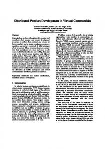
Another way to influence the opportunities for modularization is to modify the configuration and/or the interface constraints shared among the components, modules and sub-system. In order to show how integration of components and the subsequent impact on other levels of modularization, let us assume that components C11 and C12 be integrated into a new component CD, with all else the same. Notice that the total number of components comprising the module MD has decreased to two. The impact of such integration is illustrated in Figure 6 (see Appendix B-2 for numerical analysis). In this case, the integration of C11 with C12 actually increased the overall interface constraints at all levels (a movement along the curve) while reducing the opportunity for modularization to 0.90 (from 0.94) and 0.29 (from 0.43) at the module and sub-system levels respectively. Notice, however, that opportunities for modularization can still be increased by change by varying the partnership index, α. So far, the analysis has assumed that the supplier-buyer partnership resembles the one of durable-arm’s length relationships, thus α=1. Assume that the firm wants to continue to produce System A but with the new component CD. The only way the firm can sustain the same level of modularization as before, according to the model, is by changing its supplier-buyer relationships. By 16
decreasing α to 0.5, a new modularization curve is generated, and significant opportunities for modularization can be obtained.
0,97
1,00
0,95
0,94
f (δ )
0,90
0,66
α =1 0,54 0,43
α =0 .5 0,29
0,07 0,02 0,00 0,00
0,321
1,108
2,717
δ
4,00
Figure 6. Comparative results of Consolidating Components C11 and C12 into CD.
Some of these findings may be counterintuitive. According to the model, the opportunities for modularization decrease as interface constraint increases. Furthermore, the model also indicates that supplier-buyer partnerships can influence the outcome of the modularization.
6.
Discussion and Conclusion This study contributes to the new product development and supply chain
management literature in many ways. First, the concept of modularization is illustrated as a new product development strategy in the supply chain management of a firm. Second, a mathematical model is introduced to explain different characteristics of modularization at different levels of analysis: component, module, sub-system, and system levels. The model portrays the non-linear relationship between modularization and interface constraints, which is characterized by the number of components and respective interfaces. One of the main emphases is to demonstrate that a change in the interface compatibility at one level of 17
analysis can have significant impact at other levels, indicating that when analyzing modularization, the entire system should be taken into consideration. Third, the model also portrays that supplier-buyer partnerships can impact opportunities for modularization. The more interdependent the suppliers and buyers are of each other, more tradeoffs with interface constraints are allowed, suggesting that modular product design favors a more strategic type of partnership to a durable arm’s length type of relationship. Sensitivity analysis as well as the derivative functions can also be analyzed with such mathematical model. Although mathematical modeling approach allows us to theoretically examine and simulate the function in many ways, the analysis is still confined to the limited number of variables allowed by the function. The model proposed in this paper analyzed modularization in terms of two variables: the number of components and the number of interfaces shared by these components. Obviously, there are other factors that can influence the opportunities for modularization such as manufacturing capabilities, organizational designs, and competence compatibility between firms, to name a few. Different estimation methods of the variables may also lead to different results. Furthermore, the model is also restricted to systems with clear and quantifiable interfaces in which the system can be divided into sub-systems, modules, and components, such as automobiles, personal computers, bicycles, and so on. Process intensive systems such as chemical, mechanical, biochemical systems may not be applicable. Despite the limitations set by the mathematical modeling techniques, a great deal of understanding about how modularization reacts to different variables is gained. One of the purposes of the model introduced in this paper is to show that there are different levels of modularization, each portraying distinct sensitivities to interface constraints and the extent of supplier-buyer partnerships. 18
Although the model strongly suggests that there is a tradeoff between standardization and customization, it does not explicitly show such relationship. Hence, the next step towards a better understanding of the modularization function is to analyze such tradeoffs. This may lead us to gain insights to make-or-buy decision criteria. Other research topics for enriching the mathematical model presented in this paper include the validation of the model with real-world systems, and estimation of the partnership index, α.
19
REFERENCE Baily, P., Farmer, D., Jessop, D. and Jones, D. (1998). Purchasing Principles & Management, 8th edition, Financial Times Management: Pitman Publishing. Baldwin, C.Y. and Clark, K.B. (1997). “Managing in an Age of Modularity,” Harvard Business Review, September-October, 84-93. Bosdogan, K., Deyst, J., Hoult, D. and Lucas, M. (1998). “Architectural innovation in product development through early supplier integration,” R&D Management, 28, 3, 163-173. Bowersox, D.J. (1982). “Emerging from the Recession: The Role of the Distribution Manager,” Focus, 1, 2, (Jul-Aug). Chiesa, V. and Manzini, R. (1998). “Organizing for technological collaborations: a managerial perspective,” R&D Management, 28, 3, 199-212 Christensen, C.M. and Rosenbloom, R.S. (1995). “Explaining the attacker’s advantage: technological paradigms, organizational dynamics, and the value network,” Research Policy, 24, 233-257. Clark, K.B. (1989). “Project Scope and Project Performance: The Effect of Parts Strategy and Supplier Involvement on Product Development,” Management Science, 35, 10, 1247-1263. Clark, K.B. and Fujimoto, T. (1991). Product Development Performance: Strategy, Organization and Management in the World of Auto Industry. Boston, MA: Harvard Business School Press. Dowlatshahi, S. (1998). “Implementing early supplier involvement: a conceptual framework,” International Journal of Operations & Production Management, 18, 2, 143-167. Dyer, J.H., Cho, D.S. and Chu, W. (1998). “Strategic Supplier Segmentation: The Next ‘Best Practice’ in Supply Chain Management,” California Management Review, 40, 2, Winter, 57-77. Dyer, J.H. and Ouchi, W.G. (1993). “Japanese Style Business Partnerships: Giving Companies a Competitive Edge,” Sloan Management Review, (Fall), 51-63. Feitzinger, E. and Lee, H.L. (1997). “Mass Customization at Hewlett-Packard: The Power of Postponement,” Harvard Business Review, (Jan-Feb), 116-121. Fine, C.H. (1998). Clockspeed – Winning Industry Control in the Age of Temporary Advantage. Reading, MA: Perseus Books. Gilmore, J.H. and Pine II, B.J. (1997). “The Four Faces of Mass Customization,” Harvard Business Review, (Jan-Feb), 91-101 Gulati, R. (1998). “Alliances and Networks,” Strategic Management Journal, 19, 293-317. 20
Henderson, R.M. and Clark, K.B. (1990). “Architectural Innovation: The Reconfiguration of Existing Product Technologies and the Failure of Established Firms,” Administrative Science Quarterly, 35, 9-30. Hsuan, J. (1999). “Modularization in Black-Box Design: Implications for Supplier-Buyer Partnerships,” paper presented at the 1999 DRUID Winter Conference, Jan. 7-9, Holte, Denmark. Hsuan, J. (1998). Capturing Market Access Factors in R&D Management. Licentiate Thesis, Helsinki School of Economics and Business Administration. Hsuan, Juliana (1998). “Modularization and its Impact on Partnerships with Suppliers and Customers,” in of The R&D Management Conference 1998 – Technology Strategy and Strategic Alliances Proceedings, Chapter 26, Sep. 30 – Oct. 2, Avila, Spain. Kamath, R. and Liker, J. (1994). “A second look at Japanese product development,” Harvard Business Review, (Nov-Dec), 154-70. Khurana, A. and Rosenthal, S.R. (1997). “Integrating the Fuzzy Front End of New Product Development,” Sloan Management Review, (Winter), 103-120. Kotha, S. (1995). “Mass Customization: Implementing the Emerging Paradigm for Competitive Advantage,” Strategic Management Journal, 16, 21-42. Langlois, R.N. and Robertson, P.L. (1992). “Networks and innovation in a modular system: Lessons from the microcomputer and stereo component industries,” Research Policy, 21, 297-313. Lundqvist, M., Sundgren, N. and Trygg, L. (1996). “Remodularization of a Product Line: Adding Complexity to Project Management,” Journal of Product Innovations Management, 13, 311-324. Motorola 1995 Summary Annual Report. Mudambi, R. and Helper, S. (1998). “The ‘Close but Adversarial’ Model of Supplier Relations in the U.S. Auto Industry,” Strategic Management Journal, 19, 775-792. Parker, D. and Hartley, K. (1997). “The economics of partnership sourcing versus adversarial competition: a critique,” European Journal of Purchasing & Supply Management, 3, 2, 115-125. Pine II, J. (1993). Mass Customization – The New Frontier in Business Competition. Boston, MA: Harvard Business School Press. Sako, M. and Helper, S. (1998). “Determinants of trust in supplier relations: Evidence from the automotive industry in Japan and in the United States,” Journal of Economic Behavior & Organization, 34, 387-417. Sanchez, R. (1994). “Towards a Science of Strategic Product Design: System Design, Component Modularity, and Product Leveraging Strategies,” University of Illinois at Urbana-Champaign Working Paper No. 94-0124. 21
Sanchez, R. and Mahoney, J.T. (1996). “Modularity, Flexibility, and Knowledge Management in Product and Organisation Design,” Strategic Management Journal, 17, (Winter Special Issue), 63-76. Tushman, M.L. and Rosenkopf, L. (1992). “Organizational Determinants of Technological Change: Toward a Sociology of Technological Evolution,” Research in Organizational Behavior, JAI Press, Greenwich, CT, 311-347. Ulrich, K. T. and Eppinger, S. (1995). Product Design and Development. New York, NY: McGraw-Hill. Womack, J.P. and Jones, D.T. (1996). Lean Thinking: Banishing Waste and Create Wealth in Your Corporation. Touchstone Books.
22
APPENDIX A – List of Equations Variables: f(δ) δ α kc km kss wc wm wss nc nm nss δm δm’ δss δss’ δs δ(avg)
modularization function interface constraint supplier-buyer partnership index number of interfaces shared between components number of interfaces shared between modules number of interfaces shared between sub-systems interface weight of the component interface weight of the module interface weight of the sub-system number of components number of modules number of sub-systems interface constraint factor of the module carried over δm to the sub-system level interface constraint factor of the sub-system carried over δss to the system level interface constraint factor of the system aggregate value of δ at each level of modularization
f (δ ) = e − αδ
2
d f (δ ) = − 2α δ e dδ f(δ )
S
α
S
δ
f (δ )
=
=
α
;0≤α≤1 −αδ
2
d f (δ dα
)
= − α δ
2
δ d f (δ ) = − 2α δ f (δ ) d δ
2
f
(δ )
k wc = c ∑ kc m k wm = m ∑ km ss k w ss = ss ∑ kss s
δ m = nc ⋅
[∏ w ]
c m
δm ′ =
∑ [δ ]
δ ss ′ =
∑ [δ ]
m ss
ss s
23
δ ss = δ m ′ + nm ⋅ δ s = δ ss ′ + nss ⋅
[∏ w ]
m ss
[∏ w ]
ss s
Appendix B.1 – Estimation of interface constraint δ for System A
C1 C2 C3 C4 C5 C6 C7 C8 C9 C10 C11 C12 C13 C14
kc
wc
1 1 1 2 1 1 3 2 2 2 2 2 1 1
0,500 0,500 0,250 0,500 0,250 0,125 0,375 0,250 0,250 0,333 0,333 0,333 0,500 0,500
δ(avg) =
MA
nc
δm
km
wm
2
0,500
1
0,500 SSy
MB
3
0,094
1
0,500
MC
4
0,012
2
0,333
MD
3
0,111
2
0,333
ME
2
0,500
2
0,333
nm
δm '
δss
k ss
w ss
2
0,594
1,094
1
0,500
SA SSz
0,243
3
0,623
0,734
0,914
24
1
n ss
δss '
δs
2
1,828
2,328
0,500
2,328
Appendix B.2 – Estimation of interface constraint δ for System A (C11 and C12 integrated into CD)
C1 C2 C3 C4 C5 C6 C7 C8 C9 C10
kc
wc
1 1 1 2 1 1 3 2 2 2
0,500 0,500 0,250 0,500 0,250 0,125 0,375 0,250 0,250 0,500
CD
2
0,500
C13 C14
1 1
0,500 0,500
δ(avg) =
MA
nc
δm
km
wm
2
0,500
1
0,500 SSy
MB
3
0,094
1
0,500
MC
4
0,012
2
0,333
MD
2
0,500
2
0,333
ME
2
0,500
2
0,333
nm
δm '
δss
k ss
w ss
2
0,594
1,094
1
0,500
SA SSz
0,321
3
1,012
1,123
1,108
25
1
n ss
δss '
δs
2
2,217
2,717
0,500
2,717