10 Jan 2018 - symbols, the modulus can also be used in MIMO detection for improving the detection per- ... the IF receivers in [13], [16] is that, each transmit antenna needs a ... per transmit antenna and per bit-layer in higher-order modulations. ... To achieve such a nice property, with MZF the modulus matrix is carefully.
1
Modulus Zero-Forcing Detection for MIMO Channels
arXiv:1801.00947v2 [cs.IT] 10 Jan 2018
Sha Hu and Fredrik Rusek
Abstract We propose a modulus arithmetic based zero-forcing (MZF) detector for multi-input multi-output (MIMO) channels. Traditionally, a ZF detector completely eliminates interference from other symbol layers when detecting a particular symbol layer, which results in suboptimal performance due to noiseenhancement. The only constraint for application of our proposed MZF detector is that the transmitter must employ a finite cardinality M quadrature-amplitude-modulation (QAM) alphabet. With that, the modus operandi of the MZF is to allow for integer-valued interference and then remove it by modulus arithmetic operations.
Index Terms Multi-input multi-output (MIMO), modulus, zero-forcing (ZF), quadrature-amplitude-modulation (QAM), pulse-amplitude-modulation (PAM), linear minimum-mean-square-error (LMMSE), sphere-decoding (SD), lattice-reduction (LR), Lenstra-Lenstra-Lov´asz (LLL).
I. I NTRODUCTION We consider a standard multi-input multi-output (MIMO) channel model with a received signal ˜ expressed as y ˜x ˜=H ˜ + n, ˜ y
(1)
˜ x ˜ and n ˜ are the complex-valued MIMO channel, transmitted symbols and Gaussian where H, noise, respectively. The authors are with the Department of Electrical and Information Technology, Lund University, Lund, Sweden (email: {firstname.lastname}@eit.lth.se).
2
˜ is referred to as a MIMO detection problem, Given received signal model (1), detecting x which has a history that can be traced back about half a century and a review on it can be found in e.g., [1]. In general, maximum likelihood (ML) detection [2] yields optimal performance but with prohibitive complexity when the MIMO dimension and/or the input alphabet has large cardinality. Effective implementations of ML detection, such as sphere-decoding (SD) [3], [4] can significantly reduce the complexity, but not overcome an exponential complexity in the number of symbol layers CITE JALDEN’S PAPER. On the other hand, linear detectors [2] such as zeroforcing (ZF) and linear minimum-mean-square-error (LMMSE), have low complexities, but also suboptimal performances. One direction for improving linear detectors is lattice-aided-reduction (LAR) [5] based approaches, which use lattice-reduction (LR) algorithms, e.g., Lenstra-LenstraLov´asz (LLL), to find a short and nearly orthogonal basis for the lattice induced by the MIMO channel [6]. Other than the existing approaches [1], as the transmitted symbols are drawn from finite alphabets such as quadrature-amplitude-modulation (QAM) and pulse-amplitude-modulation (PAM) symbols, the modulus can also be used in MIMO detection for improving the detection performance. The modulus operation has been used in Tomlinson-Harashima precoding (THP) [7], [8] as suboptimal approximation for dirty-paper coding (DPC) [9], and recently it has also be considered in the designs of integer-forcing (IF) receives for MIMO channles [13], [15], [16]. The IF scheme in [13] requires the transmitter to employ a same lattice code [14] for each transmitted layer, which does not apply in most of current communication systems. Besides, when higher-oder modulations such as M -PAM are used, designing lattice code over ZM is challenging [14]. Simpler IF receivers dealing with linear binary codes such as turbo and LDPC are proposed in [15], [16], and the designs follow the same as in [13]. One disadvantage of the IF receivers in [13], [16] is that, each transmit antenna needs a separate encoding/decoding process, which is not the case in practical LTE systems where one codeword is split among transmit-antennas. Moreover, the IF design in [15] needs a separate encoding/decoding process per transmit antenna and per bit-layer in higher-order modulations. Another advantage is that, the receiver has to detect the linear combinations of codewords for all transmit-antennas first, followed by a matrix inversion (over a finite-field) process to recover the original codeword on each layer. To overcome these disadvantages in previous IF receiver designs, we consider a new approach to improve linear detection with modulus operation, namely, the proposed modulus ZF (MZF)
3
detection. Note that, MZF is conceptually different from previous IF receivers, although they share quite some similarities. The fundamental difference is that, with MZF, there is no encoding/decoding process needed which are implemented on a finite-filed with IF receivers to recover the transmit symbols (i.e., the linear combinations of codewords across all transmit-antennas). Alternatively, we design MZF detector such that the transmit symbols on each transmit-antenna can be recovered directly by modulating away the interferences from the remaining transmitantennas, and the symbol detection on different transmit-antenna is independent and fully in parallel. Such a principle simplifies the operation and can be well cooperated into practical systems such as LTE. To achieve such a nice property, with MZF the modulus matrix is carefully designed and optimized according to the specific modulation-order. II. P RELIMINARIES We start with reviewing the standard ZF detection. Before proceeding, without loss of gener˜ is always assumed to be a square matrix, obtained by a QR factorization or ality, the matrix H padding zero rows to the matrix if necessary. With the following definitions, ˜ ˜ ˜ R{˜ y} R{˜ x} R{n} R{H} −I{H} , x = , n = , H = , y= ˜ ˜ ˜ I{˜ y} I{˜ x} I{n} I{H} R{H}
(2)
we can rewrite (1) as a real-valued model y = Hx + n
(3)
where the K ×K channel matrix H is known to the receiver, x = [x1 . . . xK ]T contains PAM √ symbols from an alphabet A = {±1, ±3, . . . , ±( M − 1)}, and n is random Gaussian noise with a covariance matrix (N0 /2)I. As the transmit power depends on M , the signal-to-noise (SNR) is defined as SNR = 2E[|xk |2 ]/N0 .
(4)
� ˆ = QA H + y , x
(5)
The ZF detector is given by
where QA (·) denotes entry-wise quantization to the nearest point in A. This can be slightly rewritten as xˆk = QA (rk ),
1≤k≤K
4
with rk = δ k H + y
(6)
and δ k = [0| .{z . . 0} 1 0| .{z . . 0}]. k−1
K−k
For later use, we note that we may just as well replace the “1” with any arbitrary scalar value and equivalently work with rk = τ xk + wk ,
(7)
where wk is zero-mean complex Gaussian noise with variance τ 2 (N0 /2)kδ k H + k2 . Accordingly, the post-processing SNR, which is independent of τ , becomes γk =
SNR , kδ k H + k2
(8)
where SNR is defined in (4). III. D ESCRIPTION OF THE P ROPOSED MZF D ETECTION A main issue with ZF is that kδ k H + k2 in (8) is typically large and results in noise-enhancement. To combat that, we make use of the underlying idea of THP but apply it to detection, without any involvement of the transmitter. We propose to replace (6) with rk = (τ δ k + q k )H + y
(9)
where q k = [qk1 , qk2 , . . . qkK ] and qk` ∈ 2Z, i.e., the even integers. With that, rk = τ xk +
K X
qk` x` + wk ,
(10)
`=1
and the post processing SNR changes to γk =
τ 2 SNR , k(τ δ k + q k )H + k2
(11)
rather than (8). Note that (10) coincides with the received signal per user in a vector perturbation (VP) system [10], [11]. Therefore, further processing of (10) follows the same steps as those for VP. Based on (10), hard-output detection of xk from rk can be obtained based on the following property.
5
Property 1. Let y =z+α
M X
p m bm ,
m=1
where α ≥ 1, |z| < 2, and pm , (bm −1) ∈ 2Z. Then, M P (y mod 4α) − 2α, if 12 pm is odd, z= m=1 (y + 2α) mod 4α� − 2α, otherwise.
(12) �
Proof. See Appendix A.
Let us now consider α = 1 (other values are considered in Section IV-A). In view of Property 1, we see that qk` and x` in (10) qualify as pm and bm . Further, from the condition |z| < 2 in Property 1, we have that τ must be selected so that √ τ max |a| = τ ( M − 1) < 2. a∈A
To finalize the detector, we let K P (rk mod 4) − 2, if 21 qk` is odd, zk = `=1 (r + 2) mod 4� − 2, otherwise, k
(13)
(14)
which can be expressed as zk = τ xk + w ˜k , where w˜k has a complicated distribution due to the modulus operation. The detected symbol xˆk can now be obtained as xˆk = Qτ A (zk ),
(15)
where the quantization is implemented on τ A, with the definition τ A = {τ x : x ∈ A}. √ We remark that, the choice τ = 2/( M − 1) is not suitable in (13). This is so since if √ τ xk +wk = 2+�, for some small � > 0, then zk = −2+�. However, provided that τ � 2/( M −1), such wrap seldomly happens at high SNR and w˜k = wk with high probability. Observe that for constellation points xk with small magnitude, then w˜k = wk with much higher probability than for constellation points xk of large magnitude. To ensure equal error probability for all constellation points, we design τ such that: The distance from 2 to the largest constellation point in τ A is half the distance between two points in τ A.
6
Following this rule results in √
τ = 2(1−log2 (
M ))
,
(16)
√ where with out loss of generality we assume that log2 ( M ) is an integer in the rest of the paper. With that, we have that w˜k is “nearly” Gaussian at high SNR; see VP-PAPER for further details. To optimize the receiver, we should solve = arg max γk q opt k qk
= arg min k(τ δ k + q k )H + k2
(17)
qk
where elements of q k are even integers. We rewrite (17) as + + 2 q opt k = arg min kτ δ k H − q k (−H )k qk
= arg min kbk − q k Bk2 ,
(18)
qk
which is an instance of sphere detection over the integers [4], and bk = τ δ k H + ,
(19)
B = −H + .
(20)
Without any further extensions, pseudo-code for implementation of the MZF detector is given in Algorithm 1. We remind the reader that the inputs H and y to the algorithm are assumed to be real-valued, while M denotes the cardinality of the complex-valued QAM constellation. We provide a worked out example of MZF detection in Appendix B to illustrate the process. A. Some Remarks on the MZF Detection With the principle of MZF detection introduced, we have a few important remarks as follows. Remark 1. The MZF is an extension of the ZF, where the latter is the special case of the former when
opt
q − δ k q opt 2 = 0, k k
(21)
where denotes the Hadamard product. Therefore, from the perspective of post-processing SNR γk , MZF is always superior to ZF.
7
Remark 2. Following Remark 1, when (21) holds, the modulus operation degrades performance and should be removed. Remark 3. In general the minimum value achieved by q opt in (18) increases as τ decreases. k That is, for alphabets with large cardinality, the gain of MZF decreases. To resolve the issue in Remark 3 and to further improve performance, some useful extensions will be introduced in Sec. IV. B. Discussion on the Diversity-Multiplexing Trade-off (DMT) In the designs of IF receivers [13], [15], [16], the target is to directly optimize + 2 popt k = arg min kpk H k ,
(22)
pk
given the constraint that P ∈ ZK×K is full-rank1 over R, where P it the matrix comprises all vectors pk . Comparing to (17), it can be seen that, with MZF we constrain pk in (22) to be 1 pk = δ k + q k , τ
(23)
where q k comprises even integers. With (23) it holds that 1 P = I + Q, τ
(24)
where τ < 1 and the elements of Q are even integers. Therefore, with MZF, the degrees-offreedom (DoFs) in designing P is less than that of an IF receiver2 . Nevertheless, we have the following Property 2 (which is an extension of [13, Theorem 5]) that shows that, the MZF also achieves the optimal DMT [18] as IF receiver does. Therefore, from an information-theoretic perspective, the MZF detection does not scarifies much performance compared to an IF receiver, while the latter one has much higher encoding/decoding complexity. 1
The rationale behind is that, in order to have P mod p to be full-rank over Zp (to recover the codewords from their linear
combinations after decoding on Zp ), it suffices to check whether P is full-rank over R, given that the magnitudes of the elements of P are upper-bounded by a constant [17, Th. 11]. 2
However, with MZF matrix P is not required to be full-rank.
8
Property 2. For a complex-valued MIMO channel with K transmit-antennas, N ≥ K receiveantennas, and independent and identically distributed (i.i.d.) Rayleigh fading, the achievable DMT with the MZF detection3 is � r� dMZF = N 1 − , 0 ≤ r ≤ K. K
(25) �
Proof. See Appendix C. IV. E XTENSIONS OF THE MZF D ETECTION
In this section we introduce some extensions to the basic MZF detector for further improving its performance. While Extension 1 and 4 are generalizations of the basic algorithm, Extension 2 is to resolve the issue mentioned for large cardinality alphabets and improve the performance for weak bit-layers, while Extension 3 is a decision feedback version of Extension 2. A. Extension 1: A scaled modulus This first extension arises from a slight relaxation of α = 1 in the MZF detector. From Property 1, we can replace (14) as K P (rk mod 4α) − 2α, qk` is odd, if 12 zk = `=1 (r + 2α) mod 4α� − 2α, otherwise. k
(26)
This requires us to optimize, instead of (17), opt (q opt ) = arg min k(τ δ k + αq k )H + k2 . k ,α
(27)
|α|≥1, q k
Solving (27) is harder than solving (17) since it can be regarded as an instance of non-coherent sphere detection. Instead, we solve (17) first, and then plug the optimal solution into (27) and solve for the optimal α. That is, q opt is obtained with (17), and k + 2 αopt = arg min k(τ δ k + αq opt k )H k , |α|≥1
(28)
opt where we sligthly abused notation since the pair (q opt ) is in general not jointly optimal k ,α
in the sense of (27). Although Extension 3 is intuitive, the gain seems marginal according to numerical results. 3
In this case, the size of H corresponding to the real-valued model in (3) is 2N ×2K.
9
B. Extension2: Bit-wise Modulus Zero-Forcing An underlying assumption of this extension is that the bit-mapping to the symbols in A is such that the constellation has an additive structure. By this we mean that a PAM symbol xk should be of the form √ log2 ( M )
X
xk =
ukb 2b−1 ,
(29)
b=1
where ukb ∈ {±1} correspond to information bits. Using Algorithm 1, the bits ukb are determined by the output xˆk = Qτ A (zk ), with setting √
τ = 2(1−log2 (
M ))
. As M increases, τ decreases and so are the gains of MZF detection. To
resolve this for large values of M , we extend the symbol-based MZF detector in Algorithm 1 to a bit-wise version. Note that we can rewrite (10) as √ log2 ( M )
X
rk = τ
b−1
ukb 2
+
K X
qk` x` + wk .
(30)
`=1
b=1
Assuming that we are interested in the n-th bit ukn , we let x˜k =
n X
ukb 2b−1 ,
(31)
b=1
which belongs to a 2n -PAM alphabet. Setting τ (n) = 21−n in (30) yields √ log2 ( M ) 1−n
rk = 2
X
x˜k +
b−n
ukb 2
b=n+1
It can be easily seen that
1 2
Plog2 (√M ) b=n+1
+
K X
qk` x` + wk .
(32)
`=1
ukb 2b−n is an odd integer so it qualifies as a valid value
of qk` , and ukn can be detected as uˆkn = sign(zk ).
(33)
Therefore, for each bit-layer, a different value of τ is used and only a sign operation is needed for detection. Extension 2 has a complexity increment over Algorithm 1 since an optimization to find q k is needed for each bit-layer. Note that, according to Remark 2, when detecting the last bit-layer and if (21) holds, the ZF estimate shall be used for detection, while for detecting the other layers, modulus operations are still needed to cancel the transmitted bits corresponding to higher bit-layers. Psuedo-code for the MZF with this extension is summarized in Algorithm 2.
10
C. Extension 3: A decision feedback version of Extension 2 An obstacle with Extension 2 is that τ (n) decreases as n grows, and as previously mentioned, performance deteriorates. Small values of n correspond to weak bit-layers, and large n correspond to strong bit-layers. Thus, with Extension 2, predominantly the weak bit-layers can gain by the MZF, while the gain could be minuscule for strong bit-layers. A gain for weak bit-layers is important since it is typically these bit-layers that limit ultimate performance. However, we can also harvest a gain for strong bit-layers via a decision feedback mechanism. To prevent error propagation in decision feedback equalization, strong bits are typically detected first and then canceled. That option is not available for MZF, rather we detect the weakest bit-layer first and then move on to stronger ones. The method works as follows. First set n = 1 and follow Extension 2 verbatim to obtain ˆ 1 = [ˆ u u11 . . . uˆK1 ]T . For notational convenience, define y 1 = y. Now construct y2 =
1 ˆ 1) . (y − H u 2 1
(34)
ˆ 1 is correct, y 2 is described with the same MIMO channel as y 1 , but with Provided that u √ √ M /2-PAM rather than M -PAM inputs. Next, move on to n = 2 and keep τ (2) = 1. Since nor the value of τ (2) neither the channel H has changed, the optimal vector q k for n = 2 coincides with that already found for n = 1. We then have that for y 2 √ log2 ( M )
rk = uk2 +
X
b−2
ukb 2
b=3
+
K X
1 qk` (x` − uˆk1 ) + wk , 2 `=1
(35)
and uˆk2 is obtained by taking the sign of zk as in (33). We proceed by y3 =
1 ˆ 2) , (y − H u 2 2
(36)
and continue the process until all bit-layers have been detected. Similarly, according to Remark 2, whenever (21) holds, the ZF estimate shall be used. Pseudocode is provided in Algorithm 3. Extension 3 is similar to Extension 2 in the sense that, the detection for all bit-layers only needs to take the signs of zk as in (33), but it has less complexity since only one optimization of (17) is needed which is shared for all bit-layers. A drawback with Extension 3 is that, as for all decision-feedback based detectors, the processing of the bit-layers cannot be parallelized, which is however, possible with Extension 2. Another drawback is potential error-propagation at low SNRs.
11
D. Extension 4: Replacing ZF by LMMSE So far we have introduced modulus arithmetic detection using ZF, however, H + can also be replaced by other linear detectors4 such as LMMSE, which sets �−1 H + = H H HH H + N0 I .
(37)
In vector form, and with the introduction of a matrix T , the received signal after equalization is � T H + y = T x + T H + H − I x + T H + n, where T = (τ I +Q). The target of optimizing q k in this case, is to minimize the interference plus noise power that equals q˜ k = arg min k(τ δ k + q k )Ek2 ,
(38)
� � E = H + H − I, N0 H + .
(39)
qk
where
Note that, when H + is the pseudo-inverse of H such as with ZF, E degrades to B, which shows the generalization of the MZF concept. The reason for introducing Extension 4 is that, the ZF detector is suboptimal to LMMSE at low SNRs, in which case the modulus operation based on LMMSE can improve performance. Therefore, it is beneficial to use LMMSE instead of ZF. Since only H + is replaced by LMMSE equalization in Extension 4, all Algorithms 1-3 still apply verbatim. There are also many other possible variations of the MZF, but which we will not pursue any further. Next we put an interest on comparing the MZF to a traditional LAR detector. The reason is that, solving (17) involves significant complexity, and we put forth an approximated solution based on LR with less computational efforts. V. A S OLUTION BASED ON ,
AND A
C OMPARISON TO , L ATTICE R EDUCTION
Except for approximately solving (17) with LR, another reason for comparing MZF with LR detection is that, the obtained MZF allows for a direct comparison to LAR detectors. In LAR as well as the MZF, the most burdening task is to execute the LLL algorithm (or other similar algorithms), thus the complexities of LAR and MZF become virtually identical. As we will demonstrate, the detection-performance of MZF is superior in some cases. 4
This is also known as regularized perturbation in VP [10].
12
A. A quick review of LAR ¯ = HT Given (3), LAR starts by performing the LLL algorithm on H, so that we obtain H ¯ is nearly orthogonal. With z = T −1 x we have where T is unimodular and H ¯ + n. y = Hz
(40)
¯ and quantizing to the nearest integers gives Performing ZF based on H ¯ −1 y) ˆ = QZ ( H z
(41)
from which one can obtain ˆ = QA (T z ˆ ). x ¯ has been established, the remaining steps are of miniscule complexity. Clearly, once H At this point, a reasonable question is, what the relation between LAR and MZF is, and whether they are equivalent? The answers to these questions are that, they are closely related, but not equivalent. Prior to quantization in (41), we can write ¯ −1 y r=H = T −1 x + w.
(42)
Since T is unimodular, so is T −1 . On the other hand, written in vector form, (9) equals r = (τ I + Q) H −1 y = (τ I + Q) x + w.
(43)
Comparing (42) and (43) with τ = 1, we see that in both cases r equals an integer-valued matrix multiplied with the data symbols, plus noise. However, the matrix T −1 in (42) has no particular structure (besides being unimodular) so the modulus operation in (14) is not available. This makes LAR, i.e., (42) and MZF, i.e., (43) fundamentally different, as the structure of (42) requires further processing in the form of (41) while (43) allows for further processing via (14). B. An approximate solution to (17) based on LLL In (17) we have the following problem to solve q opt = arg min kb − qBk2 , q
(44)
13
where we removed the subscript k, and the vectors are row-vectors. Perform the LLL algorithm to B T so that we have ¯ = BTT . B Since B = −H + the LLL algorithm needs, similar to LAR, to be executed only once per coherence interval. We can now proceed as in the LAR case, ¯ −1 bT ) ˆ = QZ ( B z followed by ˆ )]T . q opt = [Q2Z (T z
(45)
Note that, the optimization (44) itself is also a MIMO detection problem (but only needs to run once per coherence-interval), therefore, there are also other low-complexity suboptimal algorithms to solve (44), such as using ZF or partial marginalization [12]. In the simulations, we will focus on the optimal SD and the suboptimal LLL solutions for (44), respectively. VI. N UMERICAL R ESULTS In this section, we show some numerical results of the proposed MZF detector, as well as its extensions. In all tests, we test with K ×K real-valued MIMO channels (each element is an independent and identically distributed Gaussian variable with a zero-mean and unit-variance) √ with M -PAM modulated symbols that are transfered from K/2×K/2 complex-valued MIMO channels and M -QAM modulated symbols. We simulate 50,000 channel realizations for each of the tests. A. SINR improvements In Fig. 1 we show the post-processing SNR improvements with the MZF detector using Algorithm 1, and compare to a traditional ZF detector with different PAM modulations (i.e., τ values). As can be seen, the SNRs are greatly improved, especially for low-order modulations (or the weak bit-layers of high-order modulations with Extension 2). When τ decreases, the gains become smaller. We also test the MZF with Extension 1, where we can observe only marginal gains (not shown in Fig. 1). Therefore, in the remaining tests we set α = 1.
14
1 0.9 0.8 0.7
CDF
0.6 0.5 0.4 0.3 0.2 =1 = 1/2 = 1/4
0.1 0
0
2
4
6
8
10
12
14
16
SNR gain of MZF over ZF in dB
Fig. 1.
SNR gains under real-valued 12×12 MIMO with 2-PAM, 4-PAM and 8-PAM modulations, respectively.
100
10-1
BER
10-2
10-3
ZF, bit-layer 1 ZF, bit-layer 2 MZF-SD, bit-layer 1 MZF-SD, bit-layer 2 MZF-SD-Ext.2, bit-layer 1 MZF-SD-Ext.3, bit-layer 2 ML, bit-layer 1 ML, bit-layer 2
10-4
10-5
0
5
10
15
20
25
SNR [dB]
Fig. 2.
Uncoded BER under real-valued 6×6 MIMO with 4-PAM modulation.
B. Uncoded bit-error-rate (BER) Next we show uncoded BER performance. In Fig. 2 we compare MZF with ZF and ML under 6×6 MIMO with 4-PAM modulation. The MZF uses SD to find the optimal q k . As can be seen, the MZF without extensions outperforms the ZF with more than 2 dB at 0.1% BER. With Extension 2, the BER of the first bit-layer (weaker layer) is greatly improved by more than 4 dB at 0.1% BER and outperforms the second bit-layer, which justifies the application of Extension
15
100
10-1
BER
10-2
10-3
ZF, bit-layer 1 ZF, bit-layer 2 ZF, bit-layer 3 MZF-SD-Ext.2, bit-layer 1 MZF-SD-Ext.2, bit-layer 2 ML, bit-layer 1 ML, bit-layer 2 ML, bit-layer 3
10-4
10-5 5
10
15
20
25
30
SNR [dB]
Fig. 3.
Uncoded BER under real-valued 4×4 MIMO with 8-PAM modulation.
100 ZF LAR MZF-LLL MZF-SD LMMSE MZF-SD-Ext.4
10-1
BER
10-2
10-3
10-4
10-5 0
2
4
6
8
10
12
14
16
SNR [dB]
Fig. 4.
Uncoded BER under real-valued 8×8 MIMO with 2-PAM modulation.
3. With Extension 3, where the feedbacks of the first bit-layer are used, the BER of the second bit-layer is also improved by more than 3 dB at 0.1% BER compared to MZF with Extension 2. The gaps between ZF and ML are significantly reduced by the MZF, and the slopes of BER with MZF are also much steeper than the ZF, and close to those with the ML. However, as also can be observed, the MZF has only marginal gains at low SNRs, and the decision-feedback approach performs even worse due to inaccurate feedbacks. This obstacle can be relieved by
16
using LMMSE based approaches, i.e., Extension 4. In Fig. 3 we repeat the tests in Fig. 2 under 4×4 MIMO with 8-PAM modulation, that is, three bit-layers are considered. The MZF with Extension 2 using SD is compared to ZF and ML. As already shown in Fig. 1, setting τ = 1/4 for detecting the third-layer (strongest layer) only has small gains, and the BER performance is also close to ZF and therefore are not shown in Fig. 3. Nevertheless, the BER of the first and second bit-layers are significantly boosted by MZF. As can be seen, the MZF performs around 3 dB better than the ZF at 0.1% BER for the second bit-layer, and 7 dB better for the first bit-layer. Since the weakest bit-layer usually has a stronger impact on the decoding performance, the gains for the first bit-layer is of importance. C. Comparison with LAR In Fig. 4 we compare the MZF with the LAR under 8×8 MIMO with 2-PAM modulation. The MZF uses both SD and the approximate LLL method to find the optimal q k . As can be seen, MZF outperforms LAR with more than 1.5 dB at 0.1% BER, with a similar complexity for running LLL algorithm for LR. Moreover, with Extension 4 (the LMMSE based detection), the BERs at low SNRs are also improved with the MZF which is inferior to the original ZF based MZF at high SNRs. Nevertheless, with Extension 4, the MZF is 4 dB better than a normal ZF, and more than 2dB better than a normal LMMSE detector at 0.1% BER. Another observation is that, the SD based MZF is more than 2 dB better than the LLL based MZF, which shows that optimal selection of q k is important. VII. S UMMARY We have proposed a novel modulus arithmetic based zero-forcing (MZF) detector for multiinput multi-output (MIMO) channels, with a number of possible extensions of the basic algorithm. The MZF detector shows significant gains in terms of post-processing signal-to-noise-ratio (SNR) and bit-error-rate (BER) compared to traditional linear detectors, at medium and high SNR scenarios and in particular for weak bit-layers. At low SNRs and with large cardinalities of the input alphabet, we have provided several possible extensions to improve the performance of the MZF. Finding the optimal modulus matrix itself is a burdening MIMO detection problem, but it needs to be done only once per a coherence-interval of the MIMO channel using spheredecoding (SD) or other suboptimal algorithms. In particular, with a similar complexity, MZF
17
with lattice-reduction (LR) based approaches outperforms the traditional lattice-aided-reduction (LAR) detector, which justifies its potential in MIMO detection. A PPENDIX A: P ROOF OF P ROPERTY 1 Since pm , (bm −1) ∈ 2Z, we let pm = 2˜ pm and bm = 2˜bm +1, where p˜m , ˜bm ∈ Z. Then, y = z+α
M X
p m bm
m=1
= z + 4α
M X
p˜m˜bm + 2α
m=1
Since |z| < 2 and α > 1, it holds that z +2α > 0. If
M X
p˜m .
(46)
m=1 1 2
M P
M P
pm =
m=1
p˜m is odd, we have
m=1
y mod 4α = z + 2α; Otherwise, if
M P
(47)
p˜m is even, it also holds that
m=1
(y + 2α) mod 4α = z + 2α.
(48)
Combing (47) and (48), z can be obtained as in (12). A PPENDIX B: A 4×4 EXAMPLE FOR APPLYING THE MZF
DETECTION
Below we give a 4×4 real-valued MIMO example with 4-PAM modulation to illustrate the process of MZF detection, with assuming the channel, transmitted symbol vector and received signal vector as
−6
0
−1
5
1
3
−3 −2 −1 1 −1 1 H = , x = , y = , 1 −5 −6 0 −1 15 1 −1 −3 −2 1 11 respectively. Then it can be shown that
−5
−55
30
−40
35 −59 −25 58 1 H+ = , 185 −30 40 −5 −55 25 −58 35 −59
18
and the ZF estimate of x equals ˜ ZF x
−60
309 1 = H +y = , 185 −730 −107
where only the third symbol is correctly detected. Next we use the basic MZF detection with Algorithm 1. Setting τ = 1 and run SD for optimization (17) yields an optimal Q as −2 0 Q= 0 2
0
0
0
0 . 0 −2 0 0 0 −2 0
2
We first see that, the MZF shall reuse the ZF estimates for the first and third layers based on (21). Then, we see that with Q, the post-processing SNR (assuming the noise power equals 1) for the second bit-layer (which is identical to the fourth bit-layer) is increased from 1/kδ 2 H + k = 185/47 to 1/k(δ 2 + q 2 )H + k2 = 185/27. Next we compute estimates with the MZF for the these two layers. For the second layer, according to (14) we have r2 = (δ 2 + q 2 )˜ xZF
−60
309 −1151 1 [0 1 2 0] , = = −730 185 185 −107
and z2 = (r2 mod 4) − 2 =
−7 . 38
Similarly, for the fourth layer we have r4 = (δ 4 + q 4 )˜ xZF
−60
309 −13 1 = [2 0 0 − 1] , = −730 185 185 −107
19
and z4 = (r4 mod 4) − 2 =
357 . 185
As can be seen, the MZF corrects both detections for the second and the fourth layers where the ZF fails. A PPENDIX C: P ROOF OF P ROPERTY 2 In the case where each transmit antenna encodes an independent data stream, the optimal DMT [18] is � r� dML (r) = N 1 − , 0 ≤ r ≤ K, K
(49)
which can be achieved by joint maximum likelihood (ML) decoding, while the ZF (and also the LMMSE) receiver attains a DMT r� dZF (r) = (N − K + 1) 1 − , 0 ≤ r ≤ K. (50) K ˜ has i.i.d. Rayleigh entries, H ˜ is full column rank with probability 1, and so is Since H ˜ To prove that the MZF detection can H ∈ Z2N ×2K which is the real-valued representation H. �
achieve the optimal DMT, we follows a similar proof in [13] for IF receiver, which builds on a result in [23] that showed that, uncoded signaling coupled with LR can achieve the full diversity and with a multiplexing gain of zero. We define a lattices Λ and its dual Λ∗ generated by 2N ×2K matrix H and 2K ×2N matrix H + as [19] � Λ = Hp, p ∈ Z2K , � Λ∗ = (H T )+ p, p ∈ Z2K ,
(51) (52)
respectively. From [19]–[21], the i-th successive minimum �i (Λ) of a lattice Λ is defined as the smallest length r (with respect to the Euclidean norm) such that, there are i vectors in Λ of length at most r that are linearly independent (with respect to R). By this definition, it holds that [13] �21 (Λ) = min kpH T k2 , p∈Z2K
�22K (Λ∗ ) =
min
P ∈Z2K×2K rank(P )=2K
max kpk H + k2 .
1≤k≤2K
(53) (54)
20
Then, we state the following Lemma 1, which follows the proof in [13, Appendix C]. Lemma 1. Let Λ be the lattice generated by H lattice generated by H according to (51). Then, for a sufficiently large s > 0, the successive minimum �2K (Λ) of Λ satisfies � � 2 K (2K + 3) ∗ 2 >s P(�2K (Λ ) > s) ≤ P �21 (Λ) � = P �21 (Λ) < s˜
(55) (56)
≤ −γ˜ s2N (ln s˜)1+N ,
(57)
where �21 (Λ) is the first successive minimum for Λ, and r 2K + 3 s˜ = K . s
(58)
The inequality (55) follows from [13, Lemma 4], and the equality (56) holds by switching �21 (Λ) to the other side, and the inequality (57) is a result of [13, Lemma 5] when s˜ > 0 and is sufficiently small. With the post-processing SNR γk in MZF detection in (11), we can show that for a given target rate r ln SNR, the outage probability equals P (R < r ln SNR) = P
max
Q∈2Z2K×2K
≤P
max
2K X 1 k=1
2
2K X 1
Q∈2Z2K×2K rank(Q)=2K k=1
2
! ln(1 + γk ) < r ln SNR ln(1 + γk ) < r ln SNR
≤P
max
Q∈2Z2K×2K
min γk < SNRr/K
1≤k≤2K
rank(Q)=2K
=P
2
max
min
Q∈2Z2K×2K 1≤k≤2K rank(Q)=2K
τ SNR < SNRr/K k(τ δ k + q k )H + k2
=P
min
Q∈2Z2K×2K
max k(τ δ k + q k )H + k2 > τ 2 SNR1−r/K .
1≤k≤2K
(59)
rank(Q)=2K
Using the inequality k(τ δ k + q k )H + k2 ≤ kq k H + k2 + τ 2 kδ k H + k2 ,
(60)
21
and inserting (60) back into (59) yields P (R < r ln SNR) ≤ P
min
Q∈2Z2K×2K
�
max kq k H + k2 > τ 2 SNR1−r/K
1≤k≤2K
� − kδ k H + k2
rank(Q)=2K
� � τ = P min max kpk H + k2 > SNR1−r/K − kδ k H + k2 2K× 2K 1≤k≤2K 4 P ∈Z rank(P )=2K � �� τ2 � + 2 1−r/K 2 ∗ = P �2K (Λ ) > SNR − kδ k H k , (61) 4
2
where the successive minimum �22K (Λ∗ ) is defined in (54). Comparing (61) to [13, Eq. (43)], it can be seen that the outage probability with MZF detection could be inferior to that with the IF receiver. However, the slope of the outage probability in high SNR regimes remains the same. Using Lemma 1, it holds that dMZF (r) = lim
− ln P (R < r ln SNR) ln SNR �� � � + 2 1−r/K τ2 ∗ 2 − ln P �2K (Λ ) > 4 SNR − kδ k H k
SNR→∞
= lim
SNR→∞ 2N
ln SNR �
1+N
− ln −γˆ s (ln sˆ) SNR→∞ ln SNR
≥ lim
,
(62)
where 2K sˆ = τ
s
2K + 3 SNR1−r/K − kδ k H + k2
2K ≥ τ
r
2K + 3 . SNR1−r/K
(63)
Inserting (63) into (62), it holds that r� dMZF (r) ≥ N 1 − . K �
(64)
But as the MZF detection is inferior to the ML detection, so is the DMT. Therefor, the equality in (64) holds. R EFERENCES [1] S. Yang and L. Hanzo, “Fifty years of MIMO detection: The road to large-scale MIMOs, ” IEEE Commun. Surveys & Tutorials, vol. 17, no. 4, pp. 1941-1988, Sep. 2015. [2] S. M. Kay, “Fundamentals of statistical signal processing, volume I: Estimation theory,” Prentice Hall signal processing series, 1993.
22
[3] A. Ghasemmehdi and E. Agrell, “Faster recursions in sphere decoding,” IEEE Trans. Inf. Theory, vol. 57, no. 6, pp. 3530-3536, Jun. 2011. [4] E. Agrell, T. Eriksson, A. Vardy and K. Zeger, “Closest point search in lattices,” IEEE Trans. Inf. Theory, vol. 48, no. 8, pp. 2201-2214, Aug. 2002. [5] D. Wubben, R. Bohnke, V. Kuhn and K. Kammeyer, “Near-maximum-likelihood detection of MIMO systems using MMSEbased lattice reduction,” IEEE Int. Conf. Commun. (ICC), Jun. 2004, pp. 798-802. [6] A. K. Lenstra, H. W. Lenstra and L. Lov´asz, “ Factoring polynomials with rational coefficients” Mathematische Annalen, vol. 261 no. 4, pp. 515-534, Jul. 1982. [7] M. Tomlinson, “New automatic equaliser employing modulo arithmetic,” Electronics Lett., vol. 7, no. 5, pp. 138-139, Mar. 1971. [8] H. Harashima and H. Miyakawa, “Matched-transmission technique for channels With intersymbol interference,” IEEE Trans. Commun., vol. 20, no. 4, pp. 774-780, Aug. 1972. [9] M. H. Costa, “Writing on dirty paper,” IEEE Trans. Inf. Theory, vol. 29, no. 2, pp. 439-441, May 1983. [10] B. M. Hochwald, C. B. Peel and A. L. Swindlehurst, “A vector-perturbation technique for near-capacity multiantenna multiuser communication - Part II: Perturbation,” IEEE Trans. Commun., vol. 53, no. 3, pp. 537-544, Mar. 2005. [11] J. Maurer, J. Jald´en, D. Seethaler and G. Matz, “Vector perturbation precoding revisited,” IEEE Trans. Signal Process., vol. 59, no. 1, pp. 315-328, Jan. 2011. [12] S. Hu and F. Rusek, “A soft-output MIMO detector with achievable information rate based partial marginalization,” IEEE Trans. Signal Processing, vol. 65, no.6, pp. 1622-1637, Mar. 2017. [13] J. Zhan, B. Nazer, U. Erez, and M. Gastpar, “Integer-forcing linear receivers,” IEEE Trans. Inform. Theory, vol. 60, no. 12, pp. 7661-7685, Dec. 2014. [14] S.-N. Hong and G. Caire, “Compute-and-forward strategies for cooperative distributed antenna systems,” IEEE Trans. Inform. Theory, vol. 59, no. 9, pp. 5227-5243, Sep. 2013. [15] S. H. Chae, M. Jang, and S.-K. Ah, “Multilevel coding scheme for integer-forcing MIMO receivers with binary codes”, IEEE Trans. Wireless. Commun., vol. 16, no. 8, pp. 5428-5441, Aug. 2017. [16] O. Ordentlich and U. Erez, “Achieving the gains promised by Integer-Forcing equalization with binary codes”, IEEE Conv. Elect. and Electron. Eng. in Israel (IEEEI), Nov. 2010, pp. 000703-000707. [17] B. Nazer and M. Gastpar, “Compute-and-forward: Harnessing interference through structured codes”, IEEE Trans. Inform. Theory, vol. 57, no. 10,pp. 6463-6486, Oct. 2011. [18] L. Zheng and D. N. C. Tse, “Diversity and multiplexing: A fundamental tradeoff in multiple-antenna channels, IEEE Trans. Inf. Theory,” IEEE Trans. Inform. Theory, vol. 49, no. 5, pp. 1073-1096, May 2003. [19] J. C. Lagarias, H. W. Lenstra, Jr., and C. P. Schnorr, “KorkinZolotarev bases and successive minima of a lattice and its reciprocal lattice,” Combinatorica, vol. 10, no. 4, pp. 333-348, Dec. 1990. [20] S. Lang, Introduction to Diophantine approximations, New York, NY, USA, Springer-Verlag, 1995. [21] I. Aliev and M. Henk, “Successive minima and best simultaneous Diophantine approximations,” Monatshefte Math., vol. 147, no. 2, pp. 95-101, 2006. [22] M. Taherzadeh, A. Mobasher, and A. K. Khandani, “Communication over MIMO broadcast channels using lattice-basis reduction”, IEEE Trans. Inform. Theory, vol. 53, no. 12, pp. 4567-4582, Dec. 2007. [23] M. Taherzadeh, A. Mobasher, and A. K. Khandani, “LLL reduction achieves the receive diversity in MIMO decoding”, IEEE Trans. Inform. Theory, vol. 53, no. 12, pp. 4801-4805, Dec. 2007.
23
Algorithm 1 Modulus Zero-Forcing (MZF) Algorithm H is K × K real-valued y is K × 1 real-valued 1:
M is cardinality of QAM constellation ˆ =M ODULAR ZF(H, y, M ) function x √
2:
τ = 2(1−log2 (
3:
B = −H +
M ))
Preprocessing for each coherence interval
4:
for k = 1 to K
5:
bk = τ δ k H +
6:
2 Solve : q opt k = arg min kbk − q k Bk qk
7:
end for
Executed for every channel observation
8: 9: 10:
for k = 1 to K + rk = (τ δ k + q opt k )H y
opt 2 if q opt = 0 then k −δ k q k
zk = bk y
11: 12:
else if
13:
end if
17:
21:
is odd then
zk = ((rk + 2) mod 4) − 2
16:
20:
opt `=1 qk`
else
15:
19:
PK
zk = (rk mod 4) − 2
14:
18:
1 2
end if xˆk = Qτ A (zk ) end for end function
24
Algorithm 2 MZF Algorithm with Extension 2 H is K × K real-valued y is K × 1 real-valued 1: 2:
M is cardinality of QAM constellation ˆ =M ODULAR ZFE XT 2(H, y, M ) function x √ N = log 2( M )
3:
B = −H +
4:
for n = 1 to N
5: 6:
τ (n) = 21−n end for
Preprocessing for each coherence interval
7:
for k = 1 to K
8:
bk = δ k H +
9:
for n = 1 to N
10:
bkn = τ (n)bk
11:
2 Solve : q opt k,n = arg min kbkn − q k Bk qk
12: 13:
end for end for
Executed for every channel observation
14: 15:
for k = 1 to K for n = 1 to N
opt 2 if n = N and q opt = 0, then k −δ k q k
16:
zk = bk y
17:
else
18: 19:
+ rk = (τ (n)δ k + q opt k )H y
20:
zk = (rk mod 4) − 2 end if
21:
uˆkn = sign(zk )
22: 23: 24: 25:
end for end for end function
25
Algorithm 3 MZF Algorithm with Extension 3 H is K × K real-valued y is K × 1 real-valued 1: 2: 3: 4:
M is cardinality of QAM constellation ˆ =M ODULAR ZFE XT 3(H, y, M ) function x τ =1
√ N = log2 ( M ) B = −H +
Preprocessing for each coherence interval
5:
for k = 1 to K
6:
bk = τ δ k H +
7:
2 Solve : q opt k = arg min kbk − q k Bk qk
8:
end for
Executed for every channel observation
9:
ˆ=y y
10:
for n = 1 to N
11:
ˆn = 0 u
12:
for k = 1 to K
opt 2 if q opt −δ q = 0, then k k k
13:
ˆ zk = τ δ k H + y
14:
else
15: 16:
+ ˆ rk = (τ δ k + q opt k )H y
17:
zk = (rk mod 4) − 2
18:
end if
19:
uˆkn = sign(zk )
20:
end for
21:
ˆ n = [ˆ u u1n uˆ2n . . . uˆKn ]T
22:
ˆ = (ˆ y y − H uˆn )/2
23: 24:
end for end function