MOG: Mapper on Graphs for Relationship Preserving Clustering
arXiv:1804.11242v1 [cs.SI] 3 Apr 2018
Mustafa Hajij, Bei Wang, Paul Rosen
(a) The mapper graph summary (top) along with the original graph (bottom)
(b) Edges in the mapper graph represent relationships between clusters
Fig. 1: (a) The mapper graph (top) provides a mechanism for extracting a compact and meaningful summary that captures the ”shape” and the main underlying structure of the original graph (bottom). Each node of the mapper graph represents a community or a cluster in the original graph. (b) In addition to capturing clusters in the original graph, mapper also provides the relationships among these clusters. Abstract— The interconnected nature of graphs often results in difficult to interpret clutter. Typically techniques focus on either decluttering by clustering nodes with similar properties or grouping edges with similar relationship. We propose using mapper, a powerful topological data analysis tool, to summarize the structure of a graph in a way that both clusters data with similar properties and preserves relationships. Typically, mapper operates on a given data by utilizing a scalar function defined on every point in the data and a cover for scalar function codomain. The output of mapper is a graph that summarize the shape of the space. In this paper, we outline how to use this mapper construction on an input graphs, outline three filter functions that capture important structures of the input graph, and provide an interface for interactively modifying the cover. To validate our approach, we conduct several case studies on synthetic and real world data sets and demonstrate how our method can give meaningful summaries for graphs with various complexities. Index Terms—Topological data analysis, mapper, graph clustering
1
Introduction
Graphs are a common data type, yet visualizing them remains a challenging problem. When considering node-link diagrams, the interconnectedness of the nodes causes edges to cross, which leads to visual clutter that makes understanding the structure difficult. Techniques such as edge bundling, motifs, and clustering have been proposed to reduce the visual clutter. In the case of edge bundling, decluttering occurs by grouping edges with similar relationships. For techniques such as motifs and clustering, clutter is reduced by grouping nodes with similar properties. In this work, we present a new approach to graph decluttering that clusters nodes based upon certain properties, while maintaining a strong notion of relationship. Our method relies on a topology-inspired construction called mapper [80]. Mapper is a tool from Topological Data Analysis (TDA) that provides a topological summary of the data [14]. • Mustafa Hajij is with University of South Florida. E-mail:
[email protected]. • Bei Wang is with University of Utah. E-mail:
[email protected]. • Paul Rosen is with University of South Florida. E-mail:
[email protected]. Manuscript received xx xxx. 201x; accepted xx xxx. 201x. Date of Publication xx xxx. 201x; date of current version xx xxx. 201x. For information on obtaining reprints of this article, please send e-mail to:
[email protected]. Digital Object Identifier: xx.xxxx/TVCG.201x.xxxxxxx
Thanks to its intuitive construction and its applicability on a wide variety of data-related problems, the construction of mapper has became one of the most successful tools in TDA. Mapper has been applied in many areas including visualization of high dimensional data [58], pattern recognition of point clouds [15], tracking resilience to infections [82], and many others [59, 66]. The mapper construction operates as an approximation tool of a general topological space. The construction operates by mapping the topological space via a “lens”, or a filter function, to another domain called the parametrization space. The properties of the filter and the parameterization space are then utilized to obtain an approximation of the original space that both clusters and preserves the relationship between clusters. Our approach works as follows: Starting with an undirected, weighted, or unweighted graph, a filter function is calculated per node, for example average geodesic distance, density, eigenfunctions, etc. A cover, which describes the cluster construction of mapper is selected. Finally, the mapper graph is constructed and visualized. The mapper graph, as seen in Figure 1(a), demonstrates 2 important properties. First, the nodes of the mapper graph represent clusters from the graph. Second, the edges of the mapper graph represent relationships between clusters, specifically which clusters overlap in the original graph. Furthermore, we provide an interactive mechanism for modifying the cover, in order to better explore the underlying graph structure. These features combined provide the capability to more
easily understand the structure of a graph under the “lens” of a filter function. In summary, the contributions of this paper are: • Generating a property and relationship preserving summary of graphs by applying mapper to the graph; • Enabling exploration of the structure by providing an interactive cover and mapper graph modification mechanism; • Demonstrate the capabilities of mapper on graphs using 3 different filter functions, namely, average geodesic distance, density, and eigenfunctions of the graph Laplacian; and • Case studies on synthetic and real graph data showing the effectiveness of our method at finding meaningful summaries in graphs. 2
Prior Work
We review prior work in graph visualization, node-link diagrams specifically, graph clustering, and the application of Topological Data Analysis to graphs. 2.1
Graph Visualization
For a comprehensive overview of graph visualization techniques, see [85]. We provide a brief outline of the most relevant methods for visualizing graphs using drawing node-link diagrams, which are utilized in many of popular graph visualization software applications, such as Gephi [5], Graphviz [31], and NodeXL [41]. The problem of visual clutter in graphs has been extensively studied in the literature of graph visualization [30]. It has been addressed in 3 main ways, improved node layouts, edges bundling, and alternative visual representations. The earliest graph layout method for node-link diagrams goes back to Tutte [83]. This was followed later by methods driven by linear programming [37], force-directed embeddings [34, 44], embeddings of the graph metric [36], and connectivity structures [11, 47, 49, 50]. Later methods created hybrid layouts driven by graph topology [2]. To reduce visual clutter on dense graphs, edge bundling can be used by rerouting edges with a common fate to overlap [42]. For massive graphs, hierarchical edge bundling has been utilized [35] and it scales to millions of edges, while divided edge bundling [76] tends to produce higher-quality results. Other methods such as replacing nodes with an alternative visual representation has been used in the literature of visual cluster. These methods range from variations on node-link diagrams, such as replacing nodes with modules [28] or motifs [27], to more abstract representations, such as variants of matrix diagrams [25] or the abstract displays of the graph statistics [46]. 2.2
Graph Clustering
Broadly speaking, our approach is closely related to graph clustering methods. The objective in graph clustering is to group the nodes of the graph together by taking into consideration the edge structure [74]. It is important to note that this is a different problem from clustering a set of graphs, where the structure similarity between a set of graphs is studied. Graph clustering algorithms are studied extensively. We only give a brief overview of the literature. See [1, 75] for more details. The techniques that have been used for graph clustering are very diverse. These techniques include spectral graph clustering-based methods [23, 33, 51, 87], similarity-measure based methods [81], global graph clustering methods [61, 62], random walks models [45, 71], and hierarchical graph clustering algorithms [10,13]. Some graph clustering literature is also aimed at directed graphs [12, 84]. Clustering of graph edges is studied in [20, 32]. Applications of graph clustering include community detection [38, 63, 64], analyzing the clusters of the global air transportation network [39], and scientific citation and collaboration [72].
2.3
Topological Data Analysis of Graphs
Over the last decade many concepts and tools from Topological Data Analysis have been introduced to the visualization community. Persistent homology is the most notable tool of TDA that has been used to study graphs [26, 29, 43, 68, 69]. It has been applied to study graphs in numerous applications, such as collaboration [3,17] and brain networks [18, 21, 53–56, 70]. Mapper [80] has been widely utilized in TDA for a number of applications [15, 58, 59, 66, 82]. Recently Mapper has witnessed major theoretical development that further adjudicate its use in data analysis [16, 22]. Besides being theoretically justified, mapper generalizes other topological summaries such as the Reeb graph [60], the contour tree [80], split, and joint trees. All these construction have found enormous applications in data visualization and data understanding. Mapper is also the main software developed by Ayasdi, a company that utilizes methods inspired by topological construction in applications of data science. To the best of our knowledge Mapper has not been utilized yet in the graph visualization. 3
Overview on Mapper Graph Construction
In this section, we apply the mapper algorithm to a graph and construct a multi-scale abstraction, referred to as a mapper graph, for summarization and exploration. We first introduce the mapper algorithm in its generality for a real-valued function with necessary but minimal topological notions. We then give an overview of the mapper construction pipeline for graphs. 3.1
A General Mapper Construction
Given a compact topological space X that is equipped with a real-valued function f : X → R, the mapper construction (or mapper for short) provides a general framework to study X which is parametrized with respect to f . The function f , commonly referred to as a filter function, plays the role of the lens, through which we look at the properties of the space, and different lenses provide different insights [7]. This is one of the key ideas behind mapper. Nerve. An open cover of a topological space X is a collection U = S {Ui }i∈I of open sets for some indexing set I such that i∈I Ui = X. We assume a cover is finite and each Ui is path-connected. Given a cover U = {Ui }i∈I of X, let Nrv(U T ) denote the nerve of the cover U , defined as Nrv(U ) = {σ ⊆ I | i∈σ Ui 6= 0} / . In this paper, we are only concerned with the 1-nerve, that is, the 1-dimensional skeleton of the nerve, denoted as Nrv1 (U ). Nrv1 (U ) is a graph with nodes representing the elements of U and edges representing the pairs (Ui ,U j ) of U such that Ui ∩U j 6= 0. / Mapper. Given a continuous map f : X → R where f (X) ⊆ [a, b] is equipped with a cover U = {Ui }i∈I , we write f ∗ (U ) as the cover of X obtained by considering the path-connected components of f −1 (Ui ) for each i. Given such a function f , its mapper M is defined to be the nerve of f ∗ (U ) [80], M(X, f , U ) := Nrv( f ∗ (U )). In this paper, we start by considering a function f : X → R and a cover U of f (X) ⊆ [a, b] consisting of finitely many open intervals U = {(a1 , b1 ), ..., (an , bn )}. We then use the map f to pull back the elements of U to obtain a cover of X by consider path-connected components of f −1 (ai , bi ) for each i, denoted as f ∗ (U ). We are interested in the 1-nerve of such a cover on X, denoted as M(X, f , U ) for the remaining of the paper, when its dimension is implied. There is a lot of flexibility in the construction of mapper. Fixing a space X, there are two primary parameters: a filter function f , and a cover U of its range space. Different filter functions can be used to capture different properties of the space X. That is why f is thought of as a lens from which we view the space X. On the other hand, fixing the map f and choosing different covers for its range space can be used to obtain mappers at multiple resolutions.
b
γ
b
γ Uγ β1 Uβ
β1
β2
β2
Uα α a
G (a)
α
a
(b)
(c)
(d)
(e)
Fig. 2: The pipeline for a mapper construction on a graph. (1) A weighted graph G(V, E). (2) A filter function f : V → R with a range space f (V ) = [a, b]. (3) A cover U of the range space is given by intervals Uα , Uβ and Uγ . (4) The connected components of the subgraphs induced by the node sets f −1 (Uα ), f −1 (Uβ ) and f −1 (Uγ ) form a cover of G, f ∗ (U ) = {α, β1 , β2 , γ}. (5) The 1-nerve of f ∗ (U ) is the mapper graph, whose nodes represent the connected components and edges represent the non-empty intersections between the connected components. In practice, the choice of a filter function and a cover depends highly on the space X and the property of interest. 3.2
Mapper Construction on Graphs
We now extend the general mapper construction by specifying the topological space X as a graph G. We start our pipeline with a graph G = (V, E) with positive edge weights. In the case when the graph G is unweighted we will assume that the edges are given the uniform weight equal to 1. The mapper construction on G takes as input a real-valued filter function defined on the nodes of the graph f : V → R, and a cover U = {(a1 , b1 ), ..., (an , bn )} of the range space f (V ) = [a, b]. The output is a summary, referred to as a mapper graph and denoted as M(G, f , U ). Computing a mapper on a graph is similar to the general algorithm with the following modifications. Given a graph G and an open interval Ui = (ai , bi ) that is part of the cover U , we define a subgraph Gi in G as the one induced by the node set f −1 (Ui ). Specifically, let Vi = {v ∈ V | f (v) ∈ (ai , bi )}, and Gi is a subgraph in G induced by the node set Vi . The connected components of Gi form a cover f ∗ (U ) of G, and its 1-nerve is denoted as M(G, f , U ). We explain this pipeline on Figure 2. We start with the input graph G given in Figure 2 (1). We define a scalar function f : V −→ [a, b] on every node of G as illustrated in Figure 2 (2). We then choose a cover U for [a, b]. In this case the choice of U consists of three intervals Uα , Uβ and Uγ as shown in Figure 2 (c). By a cover here we mean [a, b] ⊂ Uα ∪Uβ ∪Uγ . We then extract the connected subgraphs from G that corresponds to each interval Uα , Uβ and Uγ . Specifically, the connected subgraph that corresponds to the interval Uα is the graph labeled α in Figure 2 (d). The interval Uβ corresponds to two connected subgraphs β1 and β2 . Finally, the interval Uγ corresponds the connected subgraph β . The final mapper graph M(G, f , U ) is shown in Figure 2 (e). Each connected component corresponds to a node in mapper graph. We found 4 connected components in step (d) and so there are 4 nodes in the mapper graph. Edges in the final mapper graph are determined by the non-trivial intersection between the node sets of the connected components we found in step (d). For instance the subgraph γ shares a node with the subgraph β1 which corresponds to inserting an edge in the mapper graph between the nodes γ and β1 . Note here that the overlap between the cover elements in necessary to have edges in the final mapper graph. 4
Parameter Exploration for Mapper Graphs
The mapper graph construction relies on the choice of two parameters: a filter function and a cover. We can also treat the exploration and manipulation of these parameters as a vehicle to study and summarize the intrinsic structure of data. 4.1
Filter Functions
An interesting open research problem is how to formulate filter functions beyond a best practice or a rule of thumb [7, 8]. In practice, height
functions, distances from the barycentre of the space, surface curvature, integral geodesic distances and geodesic distances from a source point in the space have all been proposed as reasonable choices for filter functions [7]. In this section, we discuss three types of filter functions defined on the node set of a graph, as illustrated in Fig. 3. Each function is chosen to reflect specific property of interest that is intrinsic to the structure of a graph. These choices are well-justified in a sense that they have been shown successful in a wide variety of applications beyond graphs.
(a)
(b)
(c)
Fig. 3: Examples of filter functions defined on the node set of a graph. (a) AGD (orange). (b) Density estimation (green) with δ = 2. (c) The Fiedler vector (purple) of the graph Laplacian. Darker colors represent lower function values. Average Geodesic Distance. Suppose a weighted graph G = (V, E) is equipped with a geodesic distance metric d, that is, d(u, v) measures the geodesic/graph distance between two nodes u, v ∈ V . d can be computed by utilizing Dijkstra’s shortest path algorithm. The average geodesic distance, AGD : V → R, is given by AGD(v) =
1 ∑ d(v, u). |V | u∈V
This definition implies that the nodes near the center of the graph will likely have low function values, while points on the periphery will have high values. The AGD function has been used extensively in shape analysis due to its desirable prosperities in detecting and reflecting symmetry [48] based on how the function values are distributed. Therefore, the AGD as a filter function is capturing the symmetric properties of a graph, which are described by all or parts of the graph that are invariant to transformations such as reflection, rotation or scaling. The mathematical notion of automorphism, in some sense, captures the symmetry of the space as it is a structural-preserving way of mapping a space to itself. More precisely, consider a graph G as a metric space equipped with the geodesic distance, (G, d). A bijection T : V → V is called an automorphism on (G, d) if d(u, v) = d(T (u), T (v)) for every u, v ∈ V . Let Aut(G) denote the group of automorphisms on G. A function f : V → R is called an isometry invariant over Aut(G) if for every T ∈ Aut(G): f ◦ T = f . The scalar AGD is an isometry invariant scalar function. Indeed, let T be on automorphism on G, then for every v ∈ V we can verify:
AGD(T (v)) = |V1 | ∑u∈V d(T (u), T (v)) = |V1 | ∑u∈V d(u, v) = AGD(v). See Fig. 3(a) and Fig. 4(a) for examples of AGD on graphs. Density Estimation. The density estimation function [79] is given by Dδ (v) =
∑ exp(
u∈V
−d(u, v)2 ), δ
(a)
where d(u, v) is the graph distance between two nodes in the graph and δ > 0. Since Dδ is completely defined in terms of the distance d, it is not hard to see that Dδ is also isometry invariant. Dδ correlates negatively with AGD as it tends to take larger values on nodes which are close to the center, see Fig. 3(a-b) and Fig. 4(a-b) for examples. Eigenfunctions of the graph Laplacian. Let G be an undirected, weighted graph with positive edge weights w : E → R. Let C(G) be the vector space of all functions f : V −→ R. The unnormalized Laplacian of the graph G is the linear operator L : C(G) → C(G) defined by mapping f ∈ C(G) to L f , where (L f )(v) =
∑
(b)
wu,v ( f (v) − f (u)).
u∈N(v)
The eigenvectors of the Laplacian L form a rich family of scalar functions defined on G with many interesting geometric properties [52]. First, the gradient of the eigenfunctions of L tends to follow the overall shape of the data [57]; and these functions has been used in applications such as graph understand [78], segmentation [73], and spectral clustering [65]. Ordering the eigenvectors of L by the increasing value of their corresponding eigenvalues, we use eigenvectors of the second and third smallest eigenvalues of L as the filter functions, denoted as f2 and f3 . These vectors usually contain low frequency information about the graph, and they usually help retaining the shape of complex graphs. In particular, f2 is commonly referred to as the Fiedler vector [57] with desirable geometric properties [24]. For instance, the maximum and the minimum of the Fielder vector tend to occur at points in the dataset with maximum geodesic distance [19] allowing it values to spread from one end of the graph following its ”shape” to the other end. See Fig. 3(c) and Fig. 4(c) for examples. 4.1.1 Histogram of the Scalar Function Understanding the distribution of the scalar values of f can be helpful in the mapper construction. Figure 5 shows an example of the histogram of the AGD on a graph. We will illustrate later how the visual information encoded in the histogram can be utilized to optimize the choice of the cover. 4.2 The Cover Let f : V −→ [a, b] be a scalar function defined on G and let cover U be a cover of the interval [a, b] consisting of the interval U1 · · ·Un . We represent this cover visually by drawing rectangular boxes besides the histogram of the the scalar function as indicated in Figure 5. As previously stated, mapper relies on a choice of cover for the interval [a, b]. The cover choice is rather flexible but also essential to achieve effective mapper visualization. To simplify the cover choice we normalize the scalar values of f from the interval [a, b] to the unit interval [0, 1] unless otherwise specified. This simplification does not yield any essential difference to the function f . It merely simplifies our choices for the cover parameters that we will describe in this section. In our pipeline the cover is constructed in two main steps: (1) the initial cover stage; and (2) interactive cover manipulation stage. We give a detailed description of these two stages below. 4.2.1 The Initial Cover Stage The initial cover choice can be done by using the regular cover method. To obtain a regular cover of the interval [a, b] we need two parameters : n ∈ Z+ the cover resolution parameter, which is basically the number of cover elements, and ε ∈ R+ the overlap parameter, which indicates
(c)
Fig. 4: The effect of a filter function on the mapper graph construction. The original graph colored by one of the three filter functions is shown on the left; its corresponding mapper graph along with a chosen cover is shown on the right. (a) AGD. (b) Density estimation with δ = 1. (c) The Fiedler vector of the graph Laplacian. b U3
U2 U1 a Fig. 5: An example of histogram of a scalar function f : V −→ [a, b] defined on a graph. The bottom part of the histogram represent the one end of the interval, namely a, and the top part represent the other end b. Along the side of the histogram we will represent the the cover subintervals by boxes. This cover consists of three subintervals U1 , U2 and U3 . the amount of overlap between two consequent cover elements. To obtain this cover on the interval [a, b], we start by splitting the interval into n subintervals [c1 , c2 ], [c2 , c3 ], ..., [cn−1 , cn ] with equal length, such that c1 = a and cn = b. The parameter ε is then used to obtain the final cover U (n, ε) := {Ui = (ci − ε, ci+1 + ε)}n−1 i=1 for [a, b]. Choosing the parameters n and ε will have a significant impact on the final mapper output. In Figure 6 we demonstrate examples of a graph G in Figure (a) with a given AGD filter defined on it. The values of the filter AGD were normalized to [0, 1]. Figures 6 (b) to (f) show the result of the mapper graph of the graph G and the filter. In figures (b), (c) and (d) we fix the overlap parameter ε and vary the cover resolution n. On the other hand, if Figures (c), (e) and (f) we fix ε and vary n. Choosing The Parameters of The Regular Cover. Our Method does
over the shape of the output. The user can select one interval in the cover and manipulate its ends dynamically in the interface. Given an interval Ui = [ai , bi ] in the cover U , our interactive cover interface allows the following functionalities on Ui : • Shrining the interval Ui to obtain a new interval Ui0 . • Expanding interval Ui to obtain a new interval Ui0 . • Shifting interval Ui to obtain a new interval Ui0 . (a)
(b)
(c)
(d)
(e)
(f)
Fig. 6: Choosing different resolution for the mapper cover. Fixing ε and varying n in the regular cover. (a) Original graph G with a AGD filter function. (b) The mapper graph with the cover U (2, 0.1). (c) The mapper graph with the cover U (3, 0.1) (d) The mapper graph with the cover U (4, 0.1). (e) The mapper graph with the cover U (3, 0.2). (f) The mapper graph with the cover U (3, 0.3). not specify require any specific values for the parameters n and ε. Any input yields a valid mapper output graph. However, in order to achieve a more useful visualization summary, we choose the parameters n and ε based on the complexity and the size of the graph G as well as the information one desires to extract from it. If the desired mapper graph M summary is required to be small then choosing the resolution n should be chosen to be small. On the other hand, the parameter ε determines the mount of interconnection and connectivity between the nodes of the mapper graph. Larger ε values indicate more interconnection between the mapper graph. Generally speaking, for large graphs and very highly connected graph we found that smaller values of ε give a more effective visualization. In this case, we found the range [0.01, 0.1] to be sufficient for more purposes. On the other hand, for small graphs the value of ε tends to be within the range [0.1, 0.3]. Using The Histogram To Help Choose the Regular Cover Parameters. The histogram of the scalar function can be used to decide the regular cover parameters as follows. Generally speaking, an evenly distributed histogram requires lower overlap ε parameters. When the histogram is not evenly distributed, as in the case of Figure 4, we usually choose higher overlap parameter ε to achieve the desired interconnectivity between the mapper nodes. This decision is also made with consideration of the size of the original graph. 4.2.2
The Interactive Cover Manipulation Stage
The initial cover stage is sufficient for most applications. However, in certain circumstances it is useful to manipulate the cover elements individually to achieve a different and more desirable mapper graph output. For this purpose we developed an interactive cover manipulation interface to aid the cover construction and achieve maximal control
These three cases are illustrated in Figures 7. We want analyze the change that occur on a mapper graph M(G, f , U ) when a certain interval Ui = [ai , bi ] ∈ U changes to a new interval Ui0 from the above three cases. In other words, given a cover element Ui in U we want to to be able to compute the mapper graph when Ui changes to another cover element Ui0 efficiently assuming that all other mapper parameters are fixed. Recall from Section 3 that for a given interval [ai , bi ], the graph Gi is the subgraph of G that is mapped to [ai , bi ] via f . As we perform one of the operations, expansion, shrinking or shifting, on the interval [ai , bi ] the graph Gi changes to a new graph G0i . We illustrate the possible changes that occur on the mapper graph by demonstrating the changes that occur on the graph Gi . As we change the interval Ui , the connected components of Gi change by merging with other components, splitting to new components, new connected components might appear and existing ones might disappearing. Below we give a detailed description of how the above three interval operations affect the mapper graph. The Interval Ui Expands. This occur when the interval Ui = [ai , bi ] changes to an interval Ui0 = [ai − ε, bi ] or Ui0 = [ai , bi + ε] for some ε > 0. See Figure 7 (a) for an illustrative example.
(a)
(c)
(b)
(d)
Fig. 7: Figure (a) shows the case when the interval Ui shrinks, from the left to the right, or equivalently when it expands, from the right interval to the left. Figure (b) shows the effect of interval shrinking (expanding) on the mapper graph nodes. Figure (c) shows the case when the interval Ui shifts to a new interval Ui0 with the same length. (d) Shows the changes in the mapper graph nodes that occur due to the interval shift. Since Ui ⊂ Ui0 then f −1 (Ui ) ⊂ f −1 (Ui0 ) and hence the graph Gi is a subgraph of G0i . In other words, due to the expansion of the interval Ui more nodes and edges from the original graph G get added to form the graph G0i . This means that each existing connected component of Gi will remain connected in G0i potentially with more nodes and edges added to it. However, as a result of adding more nodes and edges, the following topological changes may occur to the connected components of Gi : • Multiple existing disjoint connected components of Gi might merge in G0i to produce a single connected component. This means that the corresponding nodes in the mapper graph will also get merged. See Figure 7 (a) and (b). • As a result of the expansion new connected component might also appear. This will result in the creation of a new node in the mapper graph. See Figure 7 (a) and (b). The Interval Ui Shrinks. This occurs when the interval Ui = [ai , bi ] changes to an interval Ui0 = [ai + ε, bi ] or Ui0 = [ai , bi − ε]. This is merely the dual case of the previous case. Namely, as we shrink the interval Ui into the interval Ui0 the graph G0i will be a subgraph of
the graph Gi . As a consequence an existing connected component in Gi might split into multiple connected components in G0i . On the level of the mapper graph, the corresponding node splits into multiple nodes. Moreover, certain connected components in Gi might disappear in G0i which translates into deleting the corresponding node in the mapper graph. The Interval Ui Shifts. This occurs when the interval Ui = [ai , bi ] changes to an interval Ui0 = [ai ± ε, bi ± ε]. This case can be considered as a combination of the sequence of expansion and shrinking of intervals as follows. If the shift is positive (i.e. upwards), the first step we change the interval [ai , bi ] to the interval [ai , bi + ε]. In the second step we change interval [ai , bi + ε] to the interval [ai + ε, bi + ε]. For a negative (i.e. downward) shift, we expand [ai − ε, bi ] and then shrink [ai − ε, bi − ε]. In both steps we are back to cases of expansion and shrinking discussed earlier. See Figure 7 (c) and (d) for an illustrative example. Using this capability, a given initial regular cover can be adjusted to realize a desirable “feature” in the data. For instance, Figure 24 (c) shows the circular feature in the mapper graph, capturing the corresponding ”circular feature” in the original graph. The cover was interactively manipulated, starting from the cover shown in Figure 24 (b). It is also useful to mention that the histogram of filter is useful in deciding the location of each individual interval. 5
visualization dynamically adds and removes nodes and edges based upon the approach outlined in Section 4.2.2. 5.3
Correlating the Substructures to the Original Graph
Having the mapper summary it is important to be able to extract the correspondence between the original data and the summary represented by mapper. All mapper components represented in our interface and can be selected dynamically to understand the structure encoded in the mapper graph. As components are selected, highlighting establishes the correspondence between the cover, the mapper graph elements, and the original graph. We provide the user with three mechanisms for exploration: node selection, edge selection, and cover element selection. Node Selection. Each node in the mapper graph corresponds to a connected component from the original graph. Selecting such a node, our interface recovers and highlights the original connected component from the graph. Furthermore, the cover element which generated the mapper graph node is additionally highlighted. For all selection examples, the color hues are chosen to be complimentary to the hue used for the filter function to maximize visual difference. Figure 8 illustrates an example of node selection in a given mapper graph.
Visual Design and Interaction
The goal of our design is to enable exploration of the structure of the graph. This is done by providing a linked-view interface between the original graph, a graph summary in the form of the mapper graph, and an interactive cover designer component that allows for customization of the mapper graph. 5.1
Graph Drawing
Graph Layout Method. For both the original graph and the mapper graph, we utilized a force-directed layout [34] with the BarnesHut optimization for repulsive force [4]. This approach was chosen for its interactive nature. However, our approach is ultimately agnostic of the underlying graph layout algorithm, and different layouts may improve the presentation of certain graphs. Node Coloring. As a part of the input for mapper we are given the filter function f : V −→ [a, b]. The filter function choice provides the hue: red for AGD, green for density, and purple for eigenfunctions. The scalar value is mapped to the saturation value of the color. This color scheme is used directly for the nodes of the original graph, as illustrated in Figure 3. Moreover, this map is also used to color the nodes of the mapper graph by taking the average of the filter function values in the connected component. For a given connected component, Cv , the average is |C1 | ∑u∈Cv f (u). v
Node Size. For the mapper graph, the size of the node is chosen to be proportional to the cardinality of the associated connected component, in other words |Cu |. Edge Thickness. For both graphs, edge thickness is drawn proportional to edge weight. For the mapper graph, recall that an edge [u, v] is determine by checking the intersection between Cu and Cv . For this reason, the edge weight, and thus thickness, is drawn proportional to the set intersection size, Cu ∩Cv . 5.2
Interactive Cover Designer
The interactive cover designer consists of 2 main elements. First on the left is the histogram of filter function f : V −→ [a, b]. This provides intuition as to which function values occur frequently and thus may be interesting to investigate further. The second element is the cover to the right. Each box represents a single cover element. The vertical position is its function value range, and the horizontal position is selected using the first-fit bin packing algorithm to minimize space consumption. As the cover elements are moved, expanded, or shrunk, the mapper graph
(a)
(b)
Fig. 8: Two examples of selecting a node from the mapper graph. In both cases the mapper graph is drawn on the top and the original graph is shown on the bottom. The selected node is colored blue and highlighted with an orange box in the mapper graph. This selection corresponds to the selection of the a collection of nodes in the original graph. The selection also triggers the selection of the cover element, highlighted in blue, that generated the mapper node. Edge Selection. Each edge [u, v] in the mapper graph M is determined by two connected components Cu and Cv in the original graph G. When selecting such an edge in our interface we highlight the nodes Cu ∪Cv with three different colors. The sets Cu − (Cu ∩ Cv ) and Cv − (Cu ∩ Cv ) each receive a different color, indicating the node clusters with similar properties. The intersection Cu ∩Cv receives a different color, highlighting the nodes responsible for the relationship between the clusters. Figure 9 illustrates this process. Interaction with the Cover. Giving an interval Ui from the cover U , it is desirable to know the set of mapper graph nodes u ∈ M and original graph nodes v ∈ G that are mapped to the interval. When a cover element Ui is selected, we select the nodes both f −1 (Ui ) and the nodes in the mapper graph M(G, f , U ) that represent the connected components of f −1 (Ui ). In Figure 10 we select the the interval (top left in (a), (b) and (c)), colored blue and highlighted by a blue box. Our system selects the corresponding nodes in the mapper graph (top) and in the original graphs (bottom). If the nodes of the mapper graph captured by a certain cover element needs fine tuning, the box may be dragged, expanded, or contracted. The mapper graph will update correspondingly.
example and demonstrate how mapper can be used to give insights about the relation among these clusters, something classical spectral clustering does not provide directly.
Bethel (a)
(a)
(b)
(c)
Fig. 9: (a-b) Selecting two different nodes in the mapper graph. Selecting a node (blue) in the mapper graph highlights the corresponding nodes in the original graph (also in blue). (c) Selecting an edge in the mapper graph (blue) selects the two nodes in the mapper graph that are attached to this node as well as the nodes in the original graph that are attached to the edge.
(a)
(b)
(c)
Fig. 10: Selecting an interval from the cover corresponds to selecting the nodes in the mapper graph that corresponds to that interval, as well as the nodes in the original graph. Figures (a-c) show the effect of selecting intervals and how it triggers the selection of the mapper graph and the original graph nodes. 6
Spectral Clustering and Mapper
In classical spectral clustering the eigenfunctions of the graph Laplacian can be used to obtain segmentation algorithms of the underlying graph. For instance the Fielder’s vector f2 can be used to bi-partition the graph G into two parts C1 = {v ∈ V | f2 (v) > 0} and C2 = {v ∈ V | f2 (v) ≤ 0}. Spectral partition is well-studied, and its justification can be found in many places in the literature [67]. The mapper construction that we presented here can be considered, in the trivial case, as a generalization for spectral clustering. For instance, the segmentation induced by the Fielder’s vector f2 is nothing more than the mapper graph M( f2 , G, U ) where U is the regular cover U(2, 0). Higher order eigenfunctions of the Laplacian have also been used for segmentation purposes in an analogous fashion [77]. The eigenfunctions of the graph Laplacian can be used to obtain an approximation for the graph mincut problem [86]. From this, edges in the mapper graph using the eigenfunction of the unnormalized Laplacian can be interpreted as an approximation of the relations between the graph segments obtained from the mincut problem. From this perspective mapper does not only provide a generalization of spectral clustering but also provide the connection between the clusters induced using these spectral techniques. Figure 11 illustrates the mapper graph of the USAIR 97 graph with the filter function f3 and the regular cover U(5, 0). Of course the mapper graph here is trivial and has merely 5 nodes representing the 5 clusters captured by f3 . Later in the next section, we return to this
Anchorage Int (b)
Fig. 11: The clustering induced by the eigenfunction f3 of the Laplacian on a graph can be seen as a special case of the mapper graph construction. Here the chosen cover is U(5, 0) gives 5 clusters of the graphs, two of them are highlighted in blue. These are exactly the same clusters obtained by using the spectral clustering on G using f3 . 7 Results In this section we evaluate our approach by examining mapper graph on synthetic and real datasets. 7.1 Mapper on Synthetic Data We validate our method by testing the output of the mapper graph on 20 synthetic datasets. All our graphs are generated using NetworkX [40]. Table 1 shows synthetic graphs and their corresponding mapper examples results. In each example a certain structure is emphasized via our choice of the scalar function and the cover. This structure could be symmetry, as in Figures 13, 18, and 22 or the overall shape of the graph, as in Figures 12, 17, and 23. One can observe that original graphs in Figures 12 and 17, have circular shape so here we choose the Fiedler’s vector as our choice of filter because we wanted a scalar function that can vary from one end of the graph to the other end. The mapper graph in Figure 17 looks interesting from our perspective because the original graph appears as a torus mesh and the mapper graph looks like the Reeb graph one usually have when computing Reeb graph on a torus mesh. Mapper also seems to capture the dual structure of some of some graph examples such as the cases in 21 and 14. It is worth mentioning that while Table 1 illustrates a single choice of a specific scalar function and a cover. Other choices could also be valid depending on the data and the context of the summary one wants to obtain from the graph. 7.2 Map of Science The map of science graph [9], Figure 24 (a), consists of 554 nodes and 2276 edges. Nodes in this graph represent specialties with major scientific disciplines and edges represent co-authorship of publications between those specialties. Figure 24 shows the graph with its nodes colored according to the major scientific disciplines of the node. Since this graph does not seem to exhibit obvious symmetry, our choice for the mapper graph scalar function was the eigenfunctions of the Laplacian. As mentioned earlier, the smallest eigenfunctions of the graph Laplacian can help retaining the shape of the graph. The third smallest eigenfunction of the graph Laplacian f3 was selected as it gave it retained the shape of the graph better than the Fiedler vector f2 . Figure 24 (b) shows the mapper graph calculated on the map of science graph using f3 with the regular cover parameters n = 10 and ε = 0.1. One can see from the figure that the mapper graph clearly preserves the overall structure and shape of the original graph. Moreover, the indicated mapper graph nodes capture certain super clusters in the original graph. Recall that the eigenfunctions of the unnormalized Laplacian can be used to approximate the graph mincut problem. Moreover the mincut output usually prefers isolated clusters in the graph [86]. Given the interpretation for the mapper graph using the eigenfunction of the Laplacian we provide in Section 6, the clusters shown in Figure 24 (b)
Table 1: Table of synthetics graphs. In all examples the mapper graph is shown on the top right and the original graph is shown on the bottom.
Fig. 12: Connected cavman graph. Regular cover U (5, 0.1).
Fig. 13: Lobster graph. Regular cover U (5, 0.1).
Fig. 14: Large Dorogovtsev Goltsev Mendes graph. Regular cover U (3, 0.2); density δ = 7.
Fig. 15: Large bipartite graph. Regular cover U (8, 0.15).
Fig. 16: Community graph. Regular cover U (5, 0.25).
Fig. 17: Annulus shape graph. Regular cover U (3, 0.3).
Fig. 18: Dorogovtsev Goltsev Mendes graph. Regular cover U (3, 0.3).
Fig. 19: Lollipop graph. Regular cover U (3, 0.1); density δ = 7.
Fig. 20: Small bipartite graph. Regular cover U (3, 0.4).
Fig. 21: Grid graph. Regular cover U (3, 0.1).
Fig. 22: Tree. Regular Regular cover U (3, 0.1).
Fig. 23: Ladder Graph. Regular cover U (4, 0.1).
are justified. However, it maybe desirable to obtain a mapper graph summary that captures more closely the shape and categories of the original graph.
the majority scientific discipline from the underlying cluster. For instance the nodes that are labeled 1 in the mapper graph represent the Humanities nodes in the original graph.
To illustrate that the mapper graph can be used to obtain a better representation of the original graph, we utilize the interactive cover capabilities presented in Section 5.2. The graph is shown in Figure 24 (c). In the mapper graph in Figure 24 (c) the nodes are circled to highlight
Figure 24 (c) indicates how the mapper graph in this instance gives a small introductory summary of the original graph. This summary is indicated in both the clusters and the relationship among those clusters. For instance node 9 and node 5 are branching nodes, namely these
Humanities
Biology
SocialMSciences
EarthMSciences
HealthMProfessionals
Chemical(MMechMdMCivilMEngineering
BrainMResearch
Chemistry
MedicalMSpecialties
MathMdMPhysics
InfectiousMDiseases Biotechnology
EbMEngineeringMdMCS
1
7
2
6
1
9
6
11
12
5
9
4
2
8
8
ga,
4 3
7
5
10
gb,
10
3
gc,
12 11
Fig. 24: (a) Circle of Science categories. (b) Circle of Science mapper graph using the regular cover U(10, 0.1) and the third smallest eigenfunction we obtained the mapper graph shown on the top. The shape preservation for the mapper graph of the original graph is indicated in the layout of the mapper graph and the original one. Some mapper graph nodes naturally capture clusters in the graph. (c) mapper graph using the interactive cover achieves better clustering quality and shape summary.
are nodes where the mapper graph changes its topology. Inspecting communities 8 and 6 we can see that these communities represent Chemistry and Biology. These two field merge at the node 5, which represents medical science and infectious diseases. 7.3
USAIR 97
The previous example illustrates the natural interpretation of the mapper graph nodes as clusters of the original graph. In Figures 25, we illustrate how the nodes and edges of the mapper graph show natural connection between clusters. The USAIR 97 graph consists of 332 nodes and 2126 edges [6]. The nodes represent airport and the edges represent the connection between the airports. For mapper graph setting we use the eigenfunction of the Laplacian f3 with interactive cover setting as shown in Figure 1 (a). Recall that we illustrated in Figure 11 on the same graph how the eigenfunction f3 can be used in spectral techniques to capture clusters in the graph but these techniques do not provide any relation among these clusters. Here We demonstrate how the mapper graph can affectively be used for this purpose. We start by examining the connection between mapper graph nodes 1 and 2 and the mapper graph edge [1, 2]. In Figure 25 (a), the cluster that corresponds to mapper graph node 1 is illustrated by the light and dark blue nodes, whereas the cluster that corresponds to mapper graph node 2 is represented by the nodes highlighted in dark blue and purple. Inspecting these nodes we can see that mapper graph node 1 corresponds to a cluster in the original graph that has the Bethel airport as a major airport. On the other hand the cluster that corresponds to mapper graph node 2 contains the major airport Anchorage international. The airports that are in contained in mapper graph edge [1, 2], highlighted in blue in Figure 25 (a), which are the Aniak and the St Mary’s airports. One can clearly see from the graph that these two airports represent the two major connection airports between cluster 1 and cluster 2. Note here that mapper graph edge [2, 3] is thicker than mapper graph edge [1, 2] (see Figure 1 (a)). This thickness indicated that there are more likely traffic in this mapper graph edge [2,3] than there is in [1,2]. The mapper graph nodes 2 and 3 and the mapper graph edge [2, 3] have similar interpretation as well. Note that nodes in C3 , shown in Figure 1 (a), has the major Juneau International airport. On the other hand C2 has two airports Aniak and St Mary’s. The mapper graph edge [2, 3] is larger than the previous case, but it can mainly represented by the Anachorage International airport. One can notice from Figure 25 (b) that in order to go from any airport represented by the C3 to the airports Aniak or St Mary’s, one must pass from through Anachorage International.
Finally, the mapper graph node 6 corresponds to the cluster C6 , shown in Figure 1 represents a peripheral cluster that is far away from the main bulk of the graph. The mapper graph node 6 is represented mainly by the Guam international airport. In order to pass from any airport in cluster C6 to the any airport in the main central bulk representing by mapper graph node 5 one must pass from the Honolulu International, which is contained in the original graph nodes that represent the mapper graph edge [5,6].
6
1 2
3 5 Anchorage2Int
St2Mary's Bethel Aniak
4 Honolulu2Int. Guam2Int.
(a) 1 2
6 3 5 4
St2Mary's Bethel
Anchorage2Int
Honolulu2Int. Guam2Int.
Aniak
Juneau2Int
(b)
Fig. 25: Selection edge in the mapper graph and the corresponding clusters in the original USAIR 97 graph. (a) The edge [1, 2] is selected indicating the connection between the cluster 1 that contains Bethel and the cluster 2, which contains Anchorage international. (b) The edge mapper graph [2,3] is selected and highlights in blue in the nodes in the original graph. In order to go from the cluster that contains Juneau International to the any of the airports in light blue one must pass through Anchorage international, which represents the main airport in the mapper graph edge [2,3].
8
Conclusion
We have presented a topological data analysis approach to generate a summary for a graph using the mapper construction. Our method is effective at finding clusters or communities in a graph and the relations among these clusters. The strength of our construction lies by its flexibility in the being able to capture the structure of the underlying graph on multiple scales and using different topological and symmetrical properties. Finally, in the future, we would like to explore other potential applications for mapper graph. Other than graph exploration, mapper graph can be consider as a skeleton for the underlying graph, which could be used for many other tasks, such as graph layout.
[24]
[25]
[26]
[27]
References [1] R. Agrawal, J. Gehrke, D. Gunopulos, and P. Raghavan. Automatic subspace clustering of high dimensional data for data mining applications, vol. 27. ACM, 1998. [2] D. Archambault, T. Munzner, and D. Auber. Topolayout: Multilevel graph layout by topological features. IEEE transactions on visualization and computer graphics, 13(2), 2007. [3] M. Bampasidou and T. Gentimis. Modeling collaborations with persistent homology. CoRR, abs/1403.5346, 2014. [4] J. Barnes and P. Hut. A hierarchical o (n log n) force-calculation algorithm. nature, 324(6096):446, 1986. [5] M. Bastian, S. Heymann, and M. Jacomy. Gephi: an open source software for exploring and manipulating networks. In ICWSM, pp. 361–362, 2009. [6] V. Batagelj and A. Mrvar. Pajek datasets, 2006. [7] S. Biasotti, D. Giorgi, M. Spagnuolo, and B. Falcidieno. Reeb graphs for shape analysis and applications. Theoretical Computer Science, 392:5–22, 2008. [8] S. Biasotti, S. Marini, M. Mortara, and G. Patane. An overview on properties and efficacy of topological skeletons in shape modelling. Shape Modeling International, 2003. [9] K. B¨orner, R. Klavans, M. Patek, A. M. Zoss, J. R. Biberstine, R. P. Light, V. Larivi`ere, and K. W. Boyack. Design and update of a classification system: The ucsd map of science. PloS one, 7(7):e39464, 2012. [10] U. Brandes, M. Gaertler, and D. Wagner. Experiments on graph clustering algorithms. In European Symposium on Algorithms, pp. 568–579, 2003. [11] U. Brandes and C. Pich. Eigensolver methods for progressive multidimensional scaling of large data. In Graph Drawing, pp. 42–53. Springer, 2007. [12] A. Broder, R. Kumar, F. Maghoul, P. Raghavan, S. Rajagopalan, R. Stata, A. Tomkins, and J. Wiener. Graph structure in the web. Computer networks, 33(1-6):309–320, 2000. [13] T. N. Bui, S. Chaudhuri, F. T. Leighton, and M. Sipser. Graph bisection algorithms with good average case behavior. Combinatorica, 7(2):171– 191, 1987. [14] G. Carlsson. Topology and data. Bulletin of the American Mathematical Society, 46(2):255–308, 2009. [15] G. Carlsson. Topological pattern recognition for point cloud data. Acta Numerica, 23:289–368, 2014. [16] M. Carri´ere and S. Oudot. Structure and stability of the 1-dimensional mapper. arXiv preprint arXiv:1511.05823, 2015. [17] C. J. Carstens and K. J. Horadam. Persistent homology of collaboration networks. Mathematical Problems in Engineering, 2013, 2013. [18] B. Cassidy, C. Rae, and V. Solo. Brain activity: Conditional dissimilarity and persistent homology. IEEE 12th International Symposium on Biomedical Imaging (ISBI), pp. 1356 – 1359, 2015. [19] M. K. Chung, S. Seo, N. Adluru, and H. K. Vorperian. Hot spots conjecture and its application to modeling tubular structures. In International Workshop on Machine Learning in Medical Imaging, pp. 225–232, 2011. [20] W. Cui, H. Zhou, H. Qu, P. C. Wong, and X. Li. Geometry-based edge clustering for graph visualization. IEEE Transactions on Visualization and Computer Graphics, 14(6):1277–1284, 2008. [21] Y. Dabaghian, F. M´emoli, L. Frank, and G. Carlsson. A topological paradigm for hippocampal spatial map formation using persistent homology. PLoS Computational Biology, 8(8):e1002581, 2012. [22] T. K. Dey, F. Memoli, and Y. Wang. Topological analysis of nerves, reeb spaces, mappers, and multiscale mappers. arXiv preprint arXiv:1703.07387, 2017. [23] I. S. Dhillon. Co-clustering documents and words using bipartite spectral graph partitioning. In Proceedings of the seventh ACM SIGKDD interna-
[28]
[29] [30]
[31]
[32]
[33] [34] [35]
[36] [37]
[38]
[39]
[40]
[41]
[42] [43]
[44] [45]
[46] [47]
[48]
[49]
tional conference on Knowledge discovery and data mining, pp. 269–274. ACM, 2001. C. H. Ding, X. He, H. Zha, M. Gu, and H. D. Simon. A min-max cut algorithm for graph partitioning and data clustering. IEEE International Conference on Data Mining, pp. 107–114, 2001. K. Dinkla, M. A. Westenberg, and J. J. van Wijk. Compressed adjacency matrices: untangling gene regulatory networks. IEEE Transactions on Visualization and Computer Graphics, 18(12):2457–2466, 2012. I. Donato, G. Petri, M. Scolamiero, L. Rondoni, and F. Vaccarino. Decimation of fast states and weak nodes: topological variation via persistent homology. Proceedings of the European Conference on Complex Systems, pp. 295–301, 2012. C. Dunne and B. Shneiderman. Motif simplification. Proceedings of the SIGCHI Conference on Human Factors in Computing Systems, 2013. T. Dwyer, N. H. Riche, K. Marriott, and C. Mears. Edge compression techniques for visualization of dense directed graphs. IEEE Transactions on Visualization and Computer Graphics, 19(12):2596–2605, 2013. W. E, J. Lu, and Y. Yao. The landscape of complex networks. CoRR, abs/1204.6376, 2012. G. Ellis and A. Dix. A taxonomy of clutter reduction for information visualisation. IEEE Transactions of Visualization and Computer Graphics, 13(6):1216–1223, 2007. J. Ellson, E. Gansner, L. Koutsofios, S. C. North, and G. Woodhull. Graphviz— open source graph drawing tools. Graph Drawing, pp. 483– 484, 2002. O. Ersoy, C. Hurter, F. Paulovich, G. Cantareiro, and A. Telea. Skeletonbased edge bundling for graph visualization. IEEE Transactions on Visualization and Computer Graphics, 17(12):2364–2373, 2011. M. Fiedler. Algebraic connectivity of graphs. Czechoslovak mathematical journal, 23(2):298–305, 1973. T. M. Fruchterman and E. M. Reingold. Graph drawing by force-directed placement. Software: Practice and experience, 21(11):1129–1164, 1991. E. R. Gansner, Y. Hu, S. North, and C. Scheidegger. Multilevel agglomerative edge bundling for visualizing large graphs. In IEEE Pacific Visualization Symposium, pp. 187–194, 2011. E. R. Gansner, Y. Koren, and S. North. Graph drawing by stress majorization. In Graph Drawing, pp. 239–250. Springer, 2005. E. R. Gansner, E. Koutsofios, S. C. North, and K.-P. Vo. A technique for drawing directed graphs. IEEE Transactions on Software Engineering, 19(3):214–230, 1993. M. Girvan and M. E. Newman. Community structure in social and biological networks. Proceedings of the national academy of sciences, 99(12):7821–7826, 2002. R. Guimera, S. Mossa, A. Turtschi, and L. N. Amaral. The worldwide air transportation network: Anomalous centrality, community structure, and cities’ global roles. Proceedings of the National Academy of Sciences, 102(22):7794–7799, 2005. A. Hagberg, P. Swart, and D. S Chult. Exploring network structure, dynamics, and function using networkx. Technical report, Los Alamos National Lab.(LANL), Los Alamos, NM (United States), 2008. D. Hansen, B. Shneiderman, and M. A. Smith. Analyzing social media networks with NodeXL: Insights from a connected world. Morgan Kaufmann, 2010. D. Holten and J. J. Van Wijk. Force-directed edge bundling for graph visualization. Computer Graphics Forum, 28(3):983–990, 2009. D. Horak, S. Maleti´c, and M. Rajkovi´c. Persistent homology of complex networks. Journal of Statistical Mechanics: Theory and Experiment, p. P03034, 2009. Y. Hu. Efficient, high-quality force-directed graph drawing. Mathematica Journal, 10(1):37–71, 2005. G. Jeh and J. Widom. Simrank: a measure of structural-context similarity. In Proceedings of the eighth ACM SIGKDD international conference on Knowledge discovery and data mining, pp. 538–543. ACM, 2002. S. Kairam, D. MacLean, M. Savva, and J. Heer. Graphprism: Compact visualization of network structure. In Advanced Visual Interfaces, 2012. M. Khoury, Y. Hu, S. Krishnan, and C. Scheidegger. Drawing large graphs by low-rank stress majorization. Computer Graphics Forum, 31:975–984, 2012. V. G. Kim, Y. Lipman, X. Chen, and T. Funkhouser. M¨obius transformations for global intrinsic symmetry analysis. Computer Graphics Forum, 29(5):1689–1700, 2010. Y. Koren. On spectral graph drawing. In Computing and Combinatorics, pp. 496–508. Springer, 2003.
[50] Y. Koren, L. Carmel, and D. Harel. Ace: A fast multiscale eigenvectors computation for drawing huge graphs. IEEE Symposium on Information Visualization, pp. 137–144, 2002. [51] B. Kulis, S. Basu, I. Dhillon, and R. Mooney. Semi-supervised graph clustering: a kernel approach. Machine learning, 74(1):1–22, 2009. [52] S. Lafon and A. B. Lee. Diffusion maps and coarse-graining: A unified framework for dimensionality reduction, graph partitioning, and data set parameterization. IEEE transactions on pattern analysis and machine intelligence, 28(9):1393–1403, 2006. [53] H. Lee, M. K. Chung, H. Kang, B.-N. Kim, and D. S. Lee. Computing the shape of brain networks using graph filtration and gromov-hausdorff metric. International Conference on Medical Image Computing and Computer Assisted Intervention, pp. 302–309, 2011. [54] H. Lee, M. K. Chung, H. Kang, B.-N. Kim, and D. S. Lee. Discriminative persistent homology of brain networks. IEEE International Symposium on Biomedical Imaging: From Nano to Macro, pp. 841–844, 2011. [55] H. Lee, H. Kang, M. K. Chung, B.-N. Kim, and D. S. Lee. Persistent brain network homology from the perspective of dendrogram. IEEE Transactions on Medical Imaging, 31(12):2267–2277, 2012. [56] H. Lee, H. Kang, M. K. Chung, B.-N. Kim, and D. S. Lee. Weighted functional brain network modeling via network filtration. NIPS Workshop on Algebraic Topology and Machine Learning, 2012. [57] B. L´evy. Laplace-beltrami eigenfunctions towards an algorithm that understands geometry. In IEEE International Conference on Shape Modeling and Applications, p. 13, 2006. [58] S. Liu, D. Maljovec, B. Wang, P.-T. Bremer, and V. Pascucci. Visualizing high-dimensional data: Advances in the past decade. IEEE Transactions on Visualization and Computer Graphics, 23(3):1249–1268, 2017. [59] P. Y. Lum, G. Singh, A. Lehman, T. Ishkanov, M. Vejdemo-Johansson, M. Alagappan, J. Carlsson, and G. Carlsson. Extracting insights from the shape of complex data using topology. Scientific Reports, 3, 2013. [60] E. Munch and B. Wang. Convergence between categorical representations of Reeb space and mapper. International Symposium on Computational Geometry (SOCG), 2016. [61] M. E. Newman. Properties of highly clustered networks. Physical Review E, 68(2):026121, 2003. [62] M. E. Newman. Fast algorithm for detecting community structure in networks. Physical review E, 69(6):066133, 2004. [63] M. E. Newman and M. Girvan. Mixing patterns and community structure in networks. In Statistical mechanics of complex networks, pp. 66–87. Springer, 2003. [64] M. E. Newman and M. Girvan. Finding and evaluating community structure in networks. Physical review E, 69(2):026113, 2004. [65] A. Y. Ng, M. I. Jordan, and Y. Weiss. On spectral clustering: Analysis and an algorithm. In Advances in neural information processing systems, pp. 849–856, 2002. [66] M. Nicolaua, A. J. Levine, and G. Carlsson. Topology based data analysis identifies a subgroup of breast cancers with a unique mutational profile and excellent survival. Proceedings National Academy of Sciences of the United States of America, 108(17):7265–7270, 2011. [67] J. Park, M. Jeon, and W. Pedrycz. Spectral clustering with physical intuition on spring–mass dynamics. Journal of the Franklin Institute, 351(6):3245–3268, 2014. [68] G. Petri, M. Scolamiero, I. Donato, and F. Vaccarino. Networks and cycles: A persistent homology approach to complex networks. Proceedings European Conference on Complex Systems 2012, Springer Proceedings in Complexity, pp. 93–99, 2013. [69] G. Petri, M. Scolamiero, I. Donato, and F. Vaccarino. Topological strata of weighted complex networks. PLoS ONE, 8(6):e66506, 2013. [70] V. Pirino, E. Riccomagno, S. Martinoia, and P. Massobrio. A topological study of repetitive co-activation networks in in vitro cortical assemblies. Physical Biology, 12(1), 2015. [71] P. Pons and M. Latapy. Computing communities in large networks using random walks. In International symposium on computer and information sciences, pp. 284–293. Springer, 2005. [72] S. Redner. How popular is your paper? an empirical study of the citation distribution. The European Physical Journal B-Condensed Matter and Complex Systems, 4(2):131–134, 1998. [73] M. Reuter, S. Biasotti, D. Giorgi, G. Patan´e, and M. Spagnuolo. Discrete laplace–beltrami operators for shape analysis and segmentation. Computers & Graphics, 33(3):381–390, 2009. [74] S. E. Schaeffer. Graph clustering. Computer science review, 1(1):27–64, 2007.
[75] S. E. Schaeffer. Graph clustering. Computer science review, 1(1):27–64, 2007. [76] D. Selassie, B. Heller, and J. Heer. Divided edge bundling for directional network data. IEEE Transactions on Visualization and Computer Graphics, 17(12):2354–2363, 2011. [77] A. Sharma, R. P. Horaud, D. Knossow, and E. Von Lavante. Mesh segmentation using laplacian eigenvectors and gaussian mixtures. In AAAI Fall Symposium: Manifold Learning and Its Applications, 2009. [78] D. I. Shuman, S. K. Narang, P. Frossard, A. Ortega, and P. Vandergheynst. The emerging field of signal processing on graphs: Extending highdimensional data analysis to networks and other irregular domains. IEEE Signal Processing Magazine, 30(3):83–98, 2013. [79] B. W. Silverman. Density estimation for statistics and data analysis, vol. 26. CRC press, 1986. [80] G. Singh, F. M´emoli, and G. Carlsson. Topological methods for the analysis of high dimensional data sets and 3d object recognition. Eurographics Symposium on Point-Based Graphics, 22, 2007. [81] Y. Tian, R. A. Hankins, and J. M. Patel. Efficient aggregation for graph summarization. In Proceedings of the 2008 ACM SIGMOD international conference on Management of data, pp. 567–580. ACM, 2008. [82] B. Y. Torres, J. H. M. Oliveira, A. T. Tate, P. Rath, K. Cumnock, and D. S. Schneider. Tracking resilience to infections by mapping disease space. PLoS biology, 14(4), 2016. [83] W. T. Tutte. How to draw a graph. Proceedings of the London Mathematical Society, s3-13(1):743–767, Jan 1963. doi: 10.1112/plms/s3-13.1. 743 [84] S. Virtanen. Clustering the chilean web. In Web Congress, 2003. Proceedings. First Latin American, pp. 229–231. IEEE, 2003. [85] T. Von Landesberger, A. Kuijper, T. Schreck, J. Kohlhammer, J. J. van Wijk, J.-D. Fekete, and D. W. Fellner. Visual analysis of large graphs: State-of-the-art and future research challenges. Computer graphics forum, 30(6):1719–1749, 2011. [86] U. Von Luxburg. A tutorial on spectral clustering. Statistics and computing, 17(4):395–416, 2007. [87] S. White and P. Smyth. A spectral clustering approach to finding communities in graphs. In Proceedings of the 2005 SIAM international conference on data mining, pp. 274–285. SIAM, 2005.